Embed Size (px)
Citation preview

Chapter 4
Analysis of Multiple Endpoints inClinical Trials
Ajit C. Tamhane
Northwestern University
Alex Dmitrienko
Eli Lilly and Company
4.1 Introduction
Most human diseases are characterized by multidimensional etiology andthe efficacy of an experimental treatment frequently needs to be assessed onmultiple outcome measures — commonly referred to as endpoints. There is avariety of ways in which the contribution of each endpoint can be accountedfor in the primary analysis, for example, the trial’s sponsor can treat endpointsas independent entities or as manifestations of a single underlying cause. Thefollowing examples illustrate the common approaches to analyzing multipleendpoints.
Example 1. If each endpoint independently provides a proof of efficacy, thetrial’s outcome is declared positive if at least one endpoint is associatedwith a significant improvement compared to the control. Gong, Pin-heiro and DeMets (2000) gave several examples of cardiovascular trialsin which the primary objective had two components (primary endpointand principal secondary endpoint), e.g., mortality and mortality plusmorbidity due to heart failure in the VEST trial (Cohn et al., 1998) andmortality plus cardiovascular morbidity and mortality in the PRAISE-Itrial (Packer et al., 1996).
Example 2. Another commonly used approach to defining the primary ob-jective in clinical trials with multiple endpoints is based on the devel-opment of composite endpoints. A composite endpoint can be based ona sum of multiple scores or combination of multiple events. In the caseof multiple events, a patient achieves a composite endpoint if he or sheexperiences any of the pre-specified events related to morbidity or mor-
131
© 2010 by Taylor and Francis Group, LLC
132 Multiple Testing Problems in Pharmaceutical Statistics
tality. For example, the primary objective of the Losartan InterventionFor Endpoint reduction (LIFE) trial was to study the effect of losartanon the composite endpoint of cardiovascular death, myocardial infarc-tion, and stroke (Dahlof et al., 2002).
Example 3. When the multiple endpoints are biologically related to eachother (for example, they measure different aspects of the same under-lying cause), the primary objective can be defined in terms of a com-bination of individual effects across the endpoints. The mitoxantronetrial in patients with progressive multiple sclerosis evaluated the overalleffect of five clinical measures: expanded disability status scale, ambula-tion index, number of treated relapses, time to first treated relapse andstandardized neurological status (Hartung et al., 2002). The analysiswas performed based on a multivariate approach that accounted for thecorrelations among the endpoints.
Example 4. In certain areas, a clinically meaningful effect is defined as thesimultaneous improvement in multiple measures. In this case, the pri-mary objective of a clinical trial is met if the test drug shows a significanteffect with respect to all the endpoints. Offen et al. (2007) gave a list ofmore than 15 examples in which a positive trial is defined in terms oftwo or more significant endpoints. They included clinical trials for thetreatment of migraine, Alzheimer’s disease and osteoarthritis.
Due to an increasing number of studies dealing with conditions that exhibita complex etiology, there has been much attention in the clinical trial literatureon the development of statistical methods for analyzing multiple endpoints.O’Brien’s (1984) paper ignited a flurry of research in this area and a number ofprocedures for testing multiple endpoints have been developed over the pasttwo decades. O’Neill (2006) mentions multiple endpoints as one of the keyareas for guidance development in FDA’s critical path initiative and writesthat “The many statistical methods and approaches that have been suggestedin the literature in recent years now deserve to be digested and placed in thecontext of how they can be best used in clinical trials.” The purpose of thischapter is to attempt to answer this need by giving a critical overview of thevarious procedures along with their assumptions, pros and cons, and domainsof applicability. For some other reviews of the literature on multiple endpoints,the reader is referred to Chi (1998), Comelli and Klersy (1996), Geller (2004),Huque and Sankoh (1997), Kieser, Reitmeir and Wassmer (1995), Sankoh,Huque and Dubey (1997) and Zhang, Quan, Ng and Stepanavage (1997).
This chapter is organized as follows. Section 4.2 introduces inferential goalsand main classes of multiple endpoint procedures. It is assumed in this chap-ter that all endpoints are primary or co-primary. Gatekeeping procedures thatdeal with endpoints classified into hierarchically ordered categories such asprimary and secondary will be discussed in Chapter 5. We begin with anoverview of multiple testing procedures for the assessment of the treatment’s
© 2010 by Taylor and Francis Group, LLC

Analysis of Multiple Endpoints in Clinical Trials 133
effect on each individual endpoint (at-least-one procedures) in Section 4.3.Global procedures aimed at examining the overall efficacy of the treatmentare reviewed in Section 4.4. Section 4.5 discusses all-or-none procedures arisingin clinical trials when the treatment’s efficacy needs to be demonstrated for allendpoints. Section 4.6 describes the superiority-noninferiority approach whichrequires demonstrating the treatment’s superiority on at least one endpointand noninferiority on others. Finally, Section 4.7 discusses software implemen-tation of selected procedures for testing multiple endpoints in clinical trials.
4.2 Inferential goals
To define inferential goals of multiple endpoint procedures, we will considera clinical trial with two treatment groups. The trial’s objective is to assessthe effect of the experimental treatment (hereafter referred to simply as thetreatment) on m endpoints compared to that of the control, e.g., placebo.Let δi denote an appropriate measure of the true treatment effect for the ithendpoint (e.g., mean difference, odds ratio or log hazard ratio). The efficacy ofthe treatment on the ith endpoint is assessed by testing the hypothesis of notreatment difference. The multiple testing setting gives rise to the problem ofType I error rate inflation. Depending on the trial’s objectives, this problemcan be addressed by performing a multiplicity adjustment, combining evidenceof the treatment’s effect across the endpoints (e.g., by combining multipleendpoints into a single composite endpoint) or utilizing other approaches.This section gives a brief overview of four main approaches to the analysis ofmultiple endpoints.
4.2.1 At-least-one procedures
If each multiple endpoint is independently clinically relevant (and can po-tentially be associated with its own regulatory claim), the multiple endpointproblem can be formulated as a multiple testing problem. Cardiovascular clin-ical trials listed in Example 1 in the Introduction serve as an illustration of thisapproach. In these trials the endpoints are treated as clinically independententities and the sponsor is interested in assessing the effect of the experimentaltreatment on each endpoint.
Given this structure of the primary objective, the trial is declared positiveif at least one significant effect is detected. The global hypothesis is defined asthe intersection of hypotheses for individual endpoints and the testing problemis stated as
HI =m⋂
i=1
(δi ≤ 0) versus KU =m⋃
i=1
(δi > 0). (4.1)
© 2010 by Taylor and Francis Group, LLC
134 Multiple Testing Problems in Pharmaceutical Statistics
The global hypothesis is rejected if one or more individual hypotheses of notreatment effect are demonstrated to be false. This is a prototypical multi-ple testing problem, known as the union-intersection (UI) problem (see Sec-tion 2.3.1), which requires a multiplicity adjustment. The objective of a mul-tiplicity adjustment is to control the familywise error rate (FWER),
FWER = P{Reject at least one true hypothesis},
at a designated level α by adjusting the level of each test downward. As inother clinical trial applications, FWER needs to be controlled in the strongsense; i.e., it must not be greater than α regardless of which hypotheses aretrue and which are false (Hochberg and Tamhane, 1987). Procedures thatcan be used in this multiple endpoint problem (at-least-one procedures) aredescribed in Section 4.3.
It is worth noting that the false discovery rate (FDR) proposed by Ben-jamini and Hochberg (1995) is generally not appropriate for the multiple end-point problem for the following reasons.
• FDR is suitable for testing a large number of hypotheses whereas thenumber of endpoints is generally very small.
• FDR is suitable for exploratory studies in which a less stringent require-ment of control of the proportion of false positives is acceptable. How-ever, tests for multiple endpoints are generally confirmatory in naturerequired for drug approval and labeling.
• The problem of testing multiple endpoints often has additional compli-cations such as ordered categories of endpoints, e.g., primary, co-primaryand secondary with logical restrictions, and decision rules based on testsfor superiority and noninferiority on different endpoints. The FDR ap-proach is not designed to handle such complex decision rules.
4.2.2 Global procedures
In many clinical trial applications it is desired to show that the treatmenthas an overall effect across the endpoints without necessarily a large significanteffect on any one endpoint (see Examples 2 and 3 in the Introduction).
To establish an overall treatment effect, usually a point null hypothesis ofno difference between the treatment and control is tested against a one-sidedalternative:
H∗I : δi = 0 for all i versus K∗
U : δi ≥ 0 for all i and δi > 0 for some i.(4.2)
It is well-known (O’Brien, 1984) that Hotelling’s T 2-test is inappropriatefor this problem because it is a two-sided test, and hence lacks power fordetecting one-sided alternatives necessary for showing the treatment efficacy.
© 2010 by Taylor and Francis Group, LLC
Analysis of Multiple Endpoints in Clinical Trials 135
In this case one-sided global procedures that have been proposed as alternativesto the T 2-test are more appropriate.
Global procedures are conceptually similar to composite endpoints (definedin Example 2) in that they also rely on reducing the number of dimensionsin a multiple endpoint problem by combining multiple measures into a singleone, e.g., combining tests for individual endpoints into a single test. However,unlike composite endpoints based on a sum or other simple function of individ-ual scores, global testing procedures address the interdependence of multipleendpoints, i.e., they account for the correlations among them. For a detaileddiscussion of global procedures, see Section 4.4.
4.2.3 All-or-none procedures
Another formulation of the multiple endpoint problem pertains to the re-quirement that the treatment be effective on all endpoints (see Example 4in the Introduction). This problem is referred to as the reverse multiplicityproblem by Offen et al. (2007) and represents the most stringent inferentialgoal for multiple endpoints. In mathematical terms, this is an example of anintersection-union (IU) problem introduced in Section 2.3.2. Within the IUframework, the global hypothesis is defined as the union of hypotheses cor-responding to individual endpoints and thus the testing problem is statedas
HU =m⋃
i=1
(δi ≤ 0) versus KI =m⋂
i=1
(δi > 0). (4.3)
To reject HU , one needs to show that all individual hypotheses are false (thetreatment effects for all endpoints are significant). All-or-none testing proce-dures are discussed in Section 4.5.
4.2.4 Superiority-noninferiority procedures
The hybrid superiority-noninferiority testing approach to testing multipleendpoints provides a viable alternative to the stringent all-or-none testingapproach described in Section 4.2.3. In this case, the goal is to demonstratethat the treatment is superior to the control on at least one endpoint and notinferior on all other endpoints.
To define the null and alternative hypotheses for this setting, let ηk ≥ 0denote the superiority threshold (commonly, ηk = 0) and εk > 0 denote thenoninferiority threshold for the kth endpoint. In other words, the treatmentis superior to the control on the kth endpoint if δk > ηk and noninferior ifδk > −εk, k = 1, . . . , m.
For the kth endpoint, the superiority testing problem is stated as
H(S)k : δk ≤ ηk versus K
(S)k : δk > ηk.
© 2010 by Taylor and Francis Group, LLC
136 Multiple Testing Problems in Pharmaceutical Statistics
Similarly, the noninferiority testing problem for the kth endpoint is stated as
H(N)k : δk ≤ −εk versus K
(N)k : δk > −εk.
Note that the difference between H(S)k and H
(N)k is simply a shift. Showing
superiority involves clearing a higher bar than showing noninferiority.The overall superiority testing problem is given by
H(S)I =
m⋂k=1
H(S)k versus K
(S)U =
m⋃k=1
K(S)k .
The global superiority hypothesis H(S)I is rejected if at least one H
(S)k is re-
jected. Similarly, the overall noninferiority testing problem is given by
H(N)U =
m⋃k=1
H(N)k versus K
(N)I =
m⋂k=1
K(N)k .
The global noninferiority hypothesis H(N)U is rejected if all H
(N)k are re-
jected. To combine the two global hypotheses and formulate the superiority-noninferiority testing approach, we need to consider testing the union of theglobal superiority and global noninferiority hypotheses
H(SN)U = H
(S)I ∪ H
(N)U versus K
(SN)I = K
(S)U ∩ K
(N)I .
In other words, the trial’s objective is met if there is superior efficacy for atleast one endpoint (K(S)
U ) and noninferior efficacy for all endpoints (K(N)I ).
This superiority-noninferiority testing problem becomes equivalent to the all-or-none testing problem (Section 4.2.3) if the noninferiority margins are setto 0 for all endpoints, i.e., ε1 = . . . = εm = 0. Superiority-noninferiorityprocedures are discussed in Section 4.6.
4.3 At-least-one procedures
This section describes p-value-based procedures as well as parametric (nor-mal theory) and resampling-based procedures for multiple endpoints when itis desired to demonstrate the treatment’s superiority on at least one endpoint.
4.3.1 Procedures based on univariate p-values
Frequently, different test statistics (e.g., t-statistics, log-rank statistics, chi-square statistics, etc.) are used to compare the treatment and control groupson different endpoints because of the different scales on which the endpoints
© 2010 by Taylor and Francis Group, LLC
Analysis of Multiple Endpoints in Clinical Trials 137
are measured. A standard approach to put the results of these different testson the same scale is via their p-values. Therefore p-value-based proceduresare of interest in the analysis of multiple endpoints. Section 2.6 provides adetailed description of popular multiple testing procedures based on univari-ate p-values. Here we briefly review basic procedures from that section withemphasis on issues specific to multiple endpoints. In addition, we describetwo p-value-based procedures introduced specifically for the multiple endpointproblem.
Bonferroni and related procedures
The simplest of the p-value-based procedures is the well-known Bonferroniprocedure introduced in Section 2.6.1. This procedure is known to be con-servative especially when there are many endpoints and/or they are highlycorrelated. More powerful stepwise versions of the Bonferroni procedure, e.g.,the Holm and Hochberg procedures, are also described in Section 2.6.
The basic Bonferroni procedure allocates the Type I error rate α equallyamong the endpoints. A weighted version of this procedure allows unequal al-location which is useful for unequally important endpoints, e.g., a clinical trialwith a principal secondary endpoint which may provide the basis for a newregulatory claim. The weighted Bonferroni procedure can also be employedin trials where some endpoints are adequately powered and the others areunderpowered.
As an example, consider the Carvedilol cardiovascular trials (Fisher andMoye, 1999) in which exercise capability plus quality of life served as theprimary endpoint and mortality was a key secondary endpoint. The primaryendpoint was not significant at the 0.05 level in the trials with the exercisecapability endpoint while the secondary mortality endpoint was highly sig-nificant in the combined analysis across the trials. Although the problem ofinterpreting the results of such trials is a vexing one (see O’Neill (1997) andDavis (1997) for contrasting views), we will assume, for the sake of illustra-tion, that the mortality endpoint was prospectively defined as a co-primaryendpoint.
In this case a decision rule based on the weighted Bonferroni procedurecan be set up. In the general case of m endpoints, the rule uses an additivealpha allocation scheme. Let w1, . . . , wm be positive weights representing theimportance of the endpoints such that they sum to 1. The hypothesis of notreatment effect for the ith endpoint is tested at level αi, where αi = wiα andthus
m∑i=1
αi = α.
In the Carvedilol example, a Bonferroni-based decision rule could have beenconstructed by assigning a large fraction of the Type I error rate α to the
© 2010 by Taylor and Francis Group, LLC

138 Multiple Testing Problems in Pharmaceutical Statistics
exercise capability endpoint (i.e., by choosing α1 close to α) and “spending”the rest on the mortality endpoint (α2 = α − α1).
A slightly sharpened version of this rule, termed the prospective alphaallocation scheme (PAAS) method, was proposed by Moye (2000). Assumingthat the p-values for the individual endpoints are independent, we have
m∏i=1
(1 − αi) = 1 − α.
Moye’s solution to the problem of two co-primary endpoints was to select thefraction of the Type I error rate α allocated to the primary endpoint andcalculate the significance level for the other endpoint from the above identity.Specifically, let 0 < α1 < α and
α2 = 1 − 1 − α
1 − α1.
In the context of the Carvedilol example, if α = 0.05 and α1 = 0.045, thenα2 = 0.0052, which is only marginally larger than α2 = 0.005 given by theweighted Bonferroni allocation.
Fixed-sequence procedure
Maurer, Hothorn and Lehmacher (1995) considered clinical trials in whichthe endpoints are a priori ordered (e.g., in terms of their importance). Theyapplied a fixed-sequence method that tests the ordered endpoints sequentiallyat level α as long as the test is significant and stops testing when a non-significant result is encountered. Effectively, α is unused when the procedurerejects the hypothesis of no treatment effect for an endpoint and thus it canbe carried over to the next endpoint. All α is used up when no treatmenteffect is detected with none left for the remaining endpoints. We refer to thisas the “use it or lose it” principle.
The fixed-sequence testing approach is widely used in clinical trials and en-dorsed by regulatory agencies; see, for example, the CPMP guidance documenton multiplicity issues (CPMP, 2002). As an example, this testing approachwas adopted in the adalimumab trial in patients with rheumatoid arthritis(Keystone et al., 2004). The trial included three endpoints (American Col-lege of Rheumatology response rate, modified total Sharp score and HealthAssessment Questionnaire score) that were prospectively ordered and testedsequentially. Since each test was carried out at an unadjusted α level, thisapproach helped the trial’s sponsor maximize the power of each individualtest. Note, however, that the overall power of the fixed-sequence proceduredepends heavily on the true effect size of the earlier endpoints. The power ofthe procedure is increased if the likelihood of detecting a treatment effect forthe endpoints at the beginning of the sequence is high. On the other hand, ifat least one of the earlier endpoints is underpowered, the procedure is likely
© 2010 by Taylor and Francis Group, LLC
Analysis of Multiple Endpoints in Clinical Trials 139
to stop early and miss an opportunity to evaluate potentially useful endpointslater in the sequence. To improve the power of the fixed-sequence procedure,it is critical to order the endpoints based on the expected strength of evidencebeginning with the endpoints associated with the largest effect size (Huqueand Alosh, 2008).
Fallback procedure
A useful generalization of the fixed-sequence procedure was proposed byWiens (2003). Wiens constructed the fallback procedure by allocating pre-specified fractions, w1, . . . , wm, of α to the m a priori ordered endpoints sub-ject to
m∑i=1
wi = 1.
The procedure begins with the first endpoint in the sequence which is testedat level α1 = αw1. Further, the ith endpoint is tested at level αi = αi−1 +αwi
if the previous endpoint is significant and level αi = αwi otherwise. In otherwords, if a certain test is not significant, its significance level (αi) is used upand, if it is significant, its level is carried over to the next endpoint, hence thename fallback procedure. Note that this procedure also uses the “use it or loseit” principle.
The fallback procedure is uniformly more powerful than the Bonferroniprocedure and reduces to the fixed-sequence procedure if all Type I errorrate is spent on the first endpoint in the sequence, i.e., w1 = 1 and w2 =· · · = wm = 0. The advantage of the fallback procedure is that one cancontinue testing even when the current test is not significant in contrast tothe fixed-sequence procedure which stops testing as soon as it encounters anonsignificant result.
As an illustration, consider a clinical trial with two endpoints, the first ofwhich (functional capacity endpoint) is adequately powered and the other one(mortality endpoint) is not (Wiens, 2003). Wiens computed the power of thefallback procedure in this example assuming that w1 = 0.8 and w2 = 0.2 (80%of the Type I error rate is spent on the functional capacity endpoint and 20%on the mortality endpoint) and the two-sided α = 0.05. Under this weightallocation scheme, the power for the mortality endpoint was substantiallyimproved (from 50% to 88% compared to the Bonferroni procedure with thesame set of weights) whereas the power for the functional capacity endpointwas reduced by a trivial amount (from 95% to 94%).
The overall power of the fallback procedure is heavily influenced by theeffect sizes of the ordered endpoints and the significance levels for their tests(or, equivalently, the pre-specified weights). As shown in the next section, thepower can be improved by arranging the endpoints in terms of the expectedeffect size, i.e., from the largest effect size to the smallest effect size. In ad-dition, the expected effect size can help determine the significance levels. For
© 2010 by Taylor and Francis Group, LLC
140 Multiple Testing Problems in Pharmaceutical Statistics
example, Huque and Alosh (2008) recommended defining the significance lev-els proportional to the reciprocals of the effect sizes. This choice helps increasethe power of the early tests which will, in turn, raise the significance levels forthe endpoints toward the end of the sequence.
Comparison of the fixed-sequence and fallback procedures
To assess the robustness of the fixed-sequence and fallback procedureswith respect to the monotonicity assumption, a simulation study was con-ducted. A clinical trial with two arms (treatment and placebo) was simulated.The treatment-placebo comparison was performed for three ordered endpoints(Endpoints 1, 2 and 3). The endpoints were tested sequentially, beginning withEndpoint 1, using the fixed-sequence method at the one-sided 0.025 level. Theendpoint outcomes were assumed to follow a multivariate normal distribu-tion with a compound-symmetric correlation matrix (i.e., the outcomes wereequicorrelated). The sample size per group (n = 98) was chosen to achieve 80%power for each univariate test when the true effect size is 0.4. The calculationswere performed using 10,000 replications.
The power of the fixed-sequence and fallback procedures for the three end-point tests is displayed in Table 4.1 for three values of the common correlationcoefficient (ρ = 0, 0.2 and 0.5) and three sets of endpoint-specific effect sizes,ei (i = 1, 2, 3). The following three scenarios were considered:
• Scenario 1. All tests are adequately powered, e1 = 0.4, e2 = 0.4, e3 = 0.4.
• Scenario 2. The first test is underpowered but the other tests are ade-quately powered, e1 = 0.3, e2 = 0.4, e3 = 0.4.
• Scenario 3. The first test is overpowered but the other tests are ade-quately powered, e1 = 0.5, e2 = 0.4, e3 = 0.4.
Consider first the case of a constant effect size (Scenario 1 in Table 4.1).Since each test serves as a gatekeeper for the tests placed later in the sequence,the power of the individual tests in the fixed-sequence procedure declines fairlyquickly as one progresses through the sequence. While the power of the firsttest is equal to its nominal value (80%), the power of the last test dropsto 61% when the endpoints are moderately correlated (ρ = 0.5). A greaterpower loss is observed with the decreasing correlation among the endpoints.Furthermore, the fixed-sequence procedure is quite sensitive to the assumptionthat the true ordering of the endpoints (in terms of the effect sizes) is close tothe actual ordering. If the first test is underpowered (Scenario 2), it createsa “domino effect” that supresses the power of the other tests. ComparingScenario 2 to Scenario 1, the power of the last test decreases from 61% to 46%for moderately correlated endpoints and from 51% to 35% for uncorrelatedendpoints. In general, the power of the fixed-sequence procedure is maximizedif the outcome of the first test is very likely to be significant (see Westfall andKrishen, 2001; Huque and Alosh, 2008). This property of the fixed-sequence
© 2010 by Taylor and Francis Group, LLC

Analysis of Multiple Endpoints in Clinical Trials 141
TABLE 4.1: Power of the fixed-sequence and fallbackprocedures in a clinical trial with three endpoints as a functionof the effect sizes and correlation. The fixed-sequence andfallback procedures are carried out at the one-sided 0.025 level.The weighting scheme for the fallback procedure is w1 = 0.5,w2 = 0.25 and w3 = 0.25.
Correlation Power of individual tests (%)(Endpoint 1, Endpoint 2, Endpoint 3)
Fixed-sequence procedure Fallback procedureScenario 1 (e1 = 0.4, e2 = 0.4, e3 = 0.4)
0 (79.6, 63.4, 50.8) (69.5, 72.3, 73.4)0.2 (79.6, 65.2, 54.4) (69.5, 71.7, 72.5)0.5 (79.6, 68.1, 61.0) (69.5, 70.7, 72.0)
Scenario 2 (e1 = 0.3, e2 = 0.4, e3 = 0.4)0 (54.9, 43.9, 35.2) (43.2, 68.3, 71.3)
0.2 (54.9, 46.1, 39.1) (43.2, 67.5, 70.4)0.5 (54.9, 49.4, 45.7) (43.2, 66.1, 69.5)
Scenario 3 (e1 = 0.5, e2 = 0.4, e3 = 0.4)0 (94.0, 75.0, 60.0) (89.9, 75.0, 75.0)
0.2 (94.0, 75.7, 62.4) (89.9, 74.8, 74.2)0.5 (94.0, 77.1, 67.2) (89.9, 74.7, 74.2)
procedure is illustrated in Scenario 3. It takes an overpowered test at thebeginning of the sequence to bring the power of the other tests closer to itsnominal level. For example, the power of the second test in the fixed-sequenceprocedure is only three to five percentage points lower than the nominal value(75-77% versus 80%) when the procedure successfully passes the first test 94%of the time.
Further, consider the properties of the fallback procedure based on thefollowing weighting scheme for the three tests: w1 = 0.5, w2 = 0.25 andw3 = 0.25. The power of the first test in the fallback procedure is uniformlylower across the three scenarios compared to the fixed-sequence procedure.This is due to the fact that the fallback procedure, unlike the fixed-sequenceprocedure, spends only half of the available Type I error rate on the first end-point. The remaining fraction is distributed over the other two tests, whichleads to a substantial improvement in their power in Scenarios 1 and 2. Specif-ically, the power of the second and third tests for the fallback procedure ismuch closer to the nominal level (80%) compared to the fixed-sequence pro-cedure. Note also that, in the case of the fallback procedure, the power ofindividual tests stays at a constant level or increases toward the end of thesequence in all three scenarios (even when the monotonicity assumption isviolated). Finally, while the power of tests placed later in the sequence im-proves with the increasing correlation for the fixed-sequence procedure, thefallback procedure exhibits an opposite trend. The power of the second andthird tests declines slowly as the correlation among the endpoints increases
© 2010 by Taylor and Francis Group, LLC
142 Multiple Testing Problems in Pharmaceutical Statistics
(the difference becomes very small when the first test is overpowered as inScenario 3).
Adaptive alpha allocation approach
Li and Mehrotra (2008) proposed a multiple testing procedure, which theyreferred to as the adaptive alpha allocation approach or 4A procedure. Considera clinical trial with m endpoints and assume that the endpoints are groupedinto two families. The first family includes m1 endpoints that are adequatelypowered and the second family includes m2 potentially underpowered end-points (m1 + m2 = m). The endpoints in the first family are tested using anyFWER controlling procedure at level α1 = α − ε, where ε > 0 is small, e.g.,α = 0.05 and ε = 0.005. For example, the Hochberg procedure decides thatall endpoints in the first family are significant if p(m1) ≤ α1, where p(m1) isthe maximum p-value associated with those endpoints. The endpoints in theother family are tested using any FWER controlling procedure at level α2,which is adaptively based on p(m1) as follows:
α2(p(m1)) =
{α if p(m1) ≤ α1,
min(α∗/p2
(m1), α1
)if p(m1) > α1,
where
α∗ =
{α1
(1 −√2 − α1/m1 − α/α1
)2
if α1 + α21/m1 − α3
1/m21 ≤ α,
α1(α − α1)/(m1 − α1) if α1 + α21/m1 − α3
1/m21 > α.
It should be pointed out that this derivation assumes that all the p-values areindependent. Li and Mehrotra also proposed an empirical adjustment to α∗ ifthe endpoints follow a multivariate normal distribution.
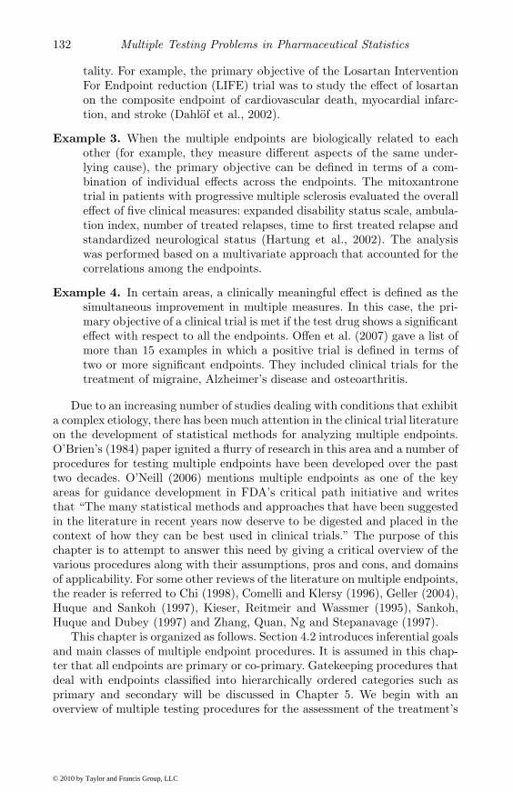
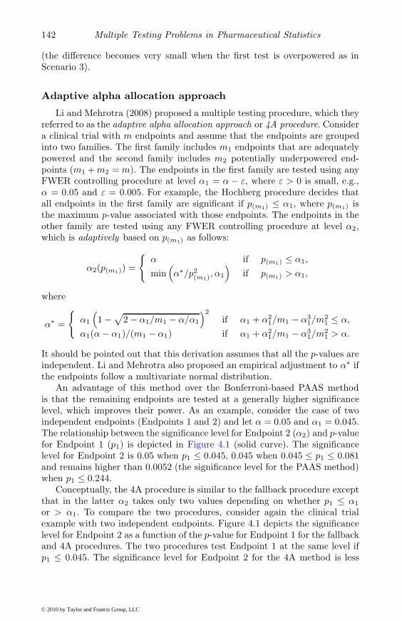
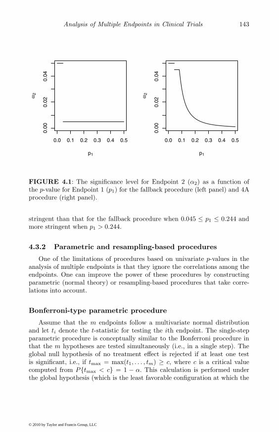
An advantage of this method over the Bonferroni-based PAAS methodis that the remaining endpoints are tested at a generally higher significancelevel, which improves their power. As an example, consider the case of twoindependent endpoints (Endpoints 1 and 2) and let α = 0.05 and α1 = 0.045.The relationship between the significance level for Endpoint 2 (α2) and p-valuefor Endpoint 1 (p1) is depicted in Figure 4.1 (solid curve). The significancelevel for Endpoint 2 is 0.05 when p1 ≤ 0.045, 0.045 when 0.045 ≤ p1 ≤ 0.081and remains higher than 0.0052 (the significance level for the PAAS method)when p1 ≤ 0.244.
Conceptually, the 4A procedure is similar to the fallback procedure exceptthat in the latter α2 takes only two values depending on whether p1 ≤ α1
or > α1. To compare the two procedures, consider again the clinical trialexample with two independent endpoints. Figure 4.1 depicts the significancelevel for Endpoint 2 as a function of the p-value for Endpoint 1 for the fallbackand 4A procedures. The two procedures test Endpoint 1 at the same level ifp1 ≤ 0.045. The significance level for Endpoint 2 for the 4A method is less
© 2010 by Taylor and Francis Group, LLC
Analysis of Multiple Endpoints in Clinical Trials 143
0.0 0.1 0.2 0.3 0.4 0.5
0.00
0.02
0.04
p1
α 2
0.0 0.1 0.2 0.3 0.4 0.5
0.00
0.02
0.04
p1
α 2
FIGURE 4.1: The significance level for Endpoint 2 (α2) as a function ofthe p-value for Endpoint 1 (p1) for the fallback procedure (left panel) and 4Aprocedure (right panel).
stringent than that for the fallback procedure when 0.045 ≤ p1 ≤ 0.244 andmore stringent when p1 > 0.244.
4.3.2 Parametric and resampling-based procedures
One of the limitations of procedures based on univariate p-values in theanalysis of multiple endpoints is that they ignore the correlations among theendpoints. One can improve the power of these procedures by constructingparametric (normal theory) or resampling-based procedures that take corre-lations into account.
Bonferroni-type parametric procedure
Assume that the m endpoints follow a multivariate normal distributionand let ti denote the t-statistic for testing the ith endpoint. The single-stepparametric procedure is conceptually similar to the Bonferroni procedure inthat the m hypotheses are tested simultaneously (i.e., in a single step). Theglobal null hypothesis of no treatment effect is rejected if at least one testis significant, i.e., if tmax = max(t1, . . . , tm) ≥ c, where c is a critical valuecomputed from P{tmax < c} = 1 − α. This calculation is performed underthe global hypothesis (which is the least favorable configuration at which the
© 2010 by Taylor and Francis Group, LLC

144 Multiple Testing Problems in Pharmaceutical Statistics
Type I error probability of this procedure is maximized over the null space).In other words, c is the (1 − α)-quantile of tmax when δ1 = . . . = δm = 0.
In general, this critical value is difficult to evaluate because the joint distri-bution of t1, . . . , tm (termed the generalized multivariate t distribution) is notknown except for the case of two endpoints (Siddiqui, 1967; Gong, Pinheiroand DeMets, 2000). Note that this distribution is different from the standardmultivariate t-distribution used in the Dunnett (1955) procedure because thedenominator of each ti uses a different error estimate, si. An additional com-plicating factor is that the joint distributions of both the numerators anddenominators of the ti statistics depend on the unknown correlation matrix.
Fallback-type parametric procedure
The main difficulty in computing critical values of the Bonferroni-typeparametric procedure is that the m test statistics are evaluated simultane-ously and one has to deal with a complicated null distribution. A stepwisemethod that examines the endpoints in a sequential manner considerably sim-plifies the process of calculating the null distributions of the test statistics andcritical values. As an illustration, we will consider the stepwise procedure formultiple endpoints proposed by Huque and Alosh (2008). This procedure is aparametric extension of the fallback procedure introduced in Section 4.3.1.
Unlike the regular fallback procedure, the parametric fallback proceduretakes into account the joint distribution of the test statistics associated withindividual endpoints, which leads to improved power for endpoints placed laterin the sequence. As before, let t1, . . . , tm denote the test statistics for the mendpoints and let w1, . . . , wm denote weights that represent the importance ofthe endpoints (the weights are positive and add up to 1). The test statisticsare assumed to follow a standard multivariate normal distribution.
The first step involves computation of critical values c1, . . . , cm and signif-icance levels γ1, . . . , γm that are defined recursively using the following equa-tions:
P (t1 ≥ c1) = αw1,
P (t1 < c1, . . . , ti−1 < ci−1, ti ≥ ci) = αwi, i = 2, . . . , m.
The probabilities are computed under the global null hypothesis. The signifi-cance levels associated with these critical values are defined as γi = 1−Φ(ci),i = 1, . . . , m, where Φ(x) is the cumulative distribution function of the stan-dard normal distribution. Given these significance levels, the testing algorithmis set up as follows. The first endpoint is tested at the γ1 level (note that γ1 =αw1 and thus the parametric procedure uses the same level for the first end-point as the regular procedure). At the ith step of the algorithm, the level isdetermined by the significance of the endpoints placed earlier in the sequence.For example, if s is the index of the last non-significant endpoint, the signif-icance level for the ith endpoint is given by max(αws+1 + . . . + αwi, γi). In
© 2010 by Taylor and Francis Group, LLC
Analysis of Multiple Endpoints in Clinical Trials 145
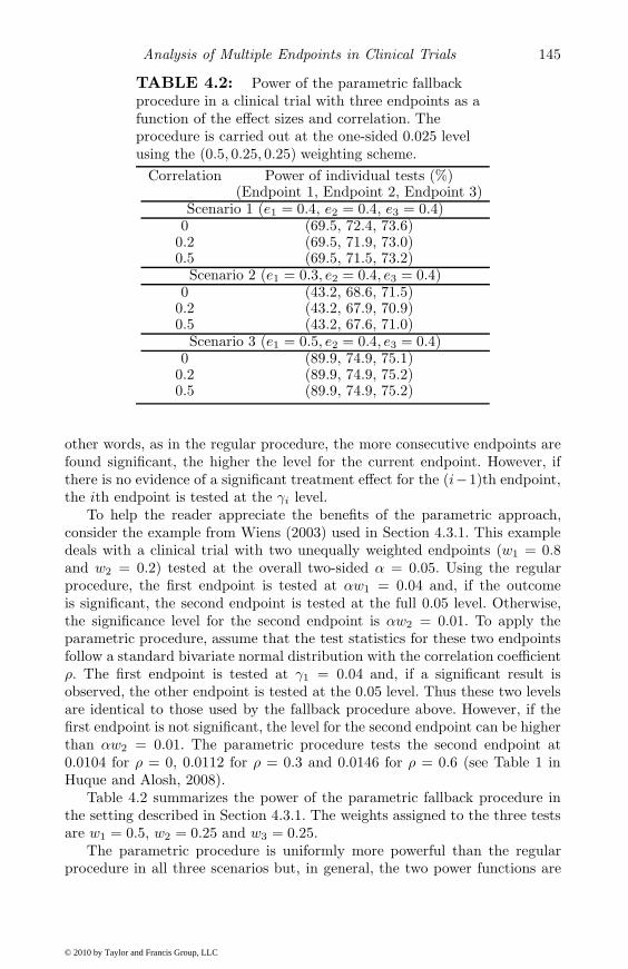
TABLE 4.2: Power of the parametric fallbackprocedure in a clinical trial with three endpoints as afunction of the effect sizes and correlation. Theprocedure is carried out at the one-sided 0.025 levelusing the (0.5, 0.25, 0.25) weighting scheme.
Correlation Power of individual tests (%)(Endpoint 1, Endpoint 2, Endpoint 3)
Scenario 1 (e1 = 0.4, e2 = 0.4, e3 = 0.4)0 (69.5, 72.4, 73.6)
0.2 (69.5, 71.9, 73.0)0.5 (69.5, 71.5, 73.2)
Scenario 2 (e1 = 0.3, e2 = 0.4, e3 = 0.4)0 (43.2, 68.6, 71.5)
0.2 (43.2, 67.9, 70.9)0.5 (43.2, 67.6, 71.0)
Scenario 3 (e1 = 0.5, e2 = 0.4, e3 = 0.4)0 (89.9, 74.9, 75.1)
0.2 (89.9, 74.9, 75.2)0.5 (89.9, 74.9, 75.2)
other words, as in the regular procedure, the more consecutive endpoints arefound significant, the higher the level for the current endpoint. However, ifthere is no evidence of a significant treatment effect for the (i−1)th endpoint,the ith endpoint is tested at the γi level.
To help the reader appreciate the benefits of the parametric approach,consider the example from Wiens (2003) used in Section 4.3.1. This exampledeals with a clinical trial with two unequally weighted endpoints (w1 = 0.8and w2 = 0.2) tested at the overall two-sided α = 0.05. Using the regularprocedure, the first endpoint is tested at αw1 = 0.04 and, if the outcomeis significant, the second endpoint is tested at the full 0.05 level. Otherwise,the significance level for the second endpoint is αw2 = 0.01. To apply theparametric procedure, assume that the test statistics for these two endpointsfollow a standard bivariate normal distribution with the correlation coefficientρ. The first endpoint is tested at γ1 = 0.04 and, if a significant result isobserved, the other endpoint is tested at the 0.05 level. Thus these two levelsare identical to those used by the fallback procedure above. However, if thefirst endpoint is not significant, the level for the second endpoint can be higherthan αw2 = 0.01. The parametric procedure tests the second endpoint at0.0104 for ρ = 0, 0.0112 for ρ = 0.3 and 0.0146 for ρ = 0.6 (see Table 1 inHuque and Alosh, 2008).
Table 4.2 summarizes the power of the parametric fallback procedure inthe setting described in Section 4.3.1. The weights assigned to the three testsare w1 = 0.5, w2 = 0.25 and w3 = 0.25.
The parametric procedure is uniformly more powerful than the regularprocedure in all three scenarios but, in general, the two power functions are
© 2010 by Taylor and Francis Group, LLC

146 Multiple Testing Problems in Pharmaceutical Statistics
quite close to each other (the difference is less than two percentage points). Theparametric procedure exhibits the same key features as the regular procedure,e.g.,
• The parametric procedure is robust with respect to the monotonicityassumption and performs well when the first test in the sequence isunderpowered.
• When the effect sizes across the tests are comparable, the power ofindividual tests improves toward the end of the sequence.
• The power of tests later in the sequence declines with increasing corre-lation.
Additional simulations performed by Huque and Alosh (2008) for the caseof two hypotheses demonstrated that the power of the parametric procedureis comparable to that of the regular procedure when the test statistics areuncorrelated or effect sizes are equal regardless of the weighting scheme. Thepower advantage of the parametric procedure for the second test increases withthe increasing correlation when the effect size of the second test is greater thanthat of the first test.
Resampling-based procedures
Given the challenges associated with single-step parametric proceduresfor multiple endpoints (the joint distribution of the test statistics dependson an unknown correlation matrix), one can consider an alternative approachthat uses the resampling-based methodology developed by Westfall and Young(1993). This alternative was explored by Reitmeir and Wassmer (1999) whointroduced resampling-based versions of several single-step and stepwise proce-dures, e.g., Bonferroni and Hommel procedures, in the context of the multipleendpoint problem.
Along the lines of the general resampling-based method (see Section 2.8 fora detailed description of resampling-based procedures), Reitmeir and Wass-mer proposed to estimate the joint distribution of the test statistics underthe global null hypothesis using the bootstrap. Beginning with any multipletest, a resampling-based at-least-one procedure can be constructed using thefollowing algorithm:
• Let pi be the p-value for the ith endpoint, i = 1, . . . , m (this p-value iscomputed using a selected test).
• Generate K bootstrap samples (draw random samples with replacementof the same size as the original samples). Let pi(k) be the treatmentcomparison p-value for the ith endpoint, which is computed from the kthbootstrap run using the selected test, i = 1, . . . , m and k = 1, . . . , K.
© 2010 by Taylor and Francis Group, LLC
Analysis of Multiple Endpoints in Clinical Trials 147
• Define the bootstrap multiplicity adjusted p-value for the ith endpointas the proportion of bootstrap runs in which pi(k) ≤ pi, 1, . . . , m.
The treatment effect for the ith endpoint is significant if the bootstrap mul-tiplicity adjusted p-value is no greater than the pre-specified familywise errorrate α. Reitmeir and Wassmer showed via simulations that the resampling-based tests for the multiple endpoint problem resulted in a consistent powergain compared to the original tests. The improvement in power was rathersmall for the Bonferroni test; however, a substantially larger gain was ob-served for some other tests, e.g., the Hommel test.
4.4 Global testing procedures
An important property of global testing procedures is that they combineevidence of treatment effect across several endpoints and thus they are morepowerful than procedures for individual endpoints (provided the treatmenteffects are consistent across the endpoints). In this section we first considerprocedures for the goal of demonstrating overall efficacy of the treatment andthen describe inferences for individual endpoints when the global assessmentproduces a significant result.
4.4.1 Normal theory model
Global testing procedures considered in this section (with a few exceptionssuch as the global rank-sum procedure introduced by O’Brien, 1984) assumethe normal theory model described below.
Consider a two-arm clinical trial with a parallel-group design in which thetreatment group (Group 1) is tested versus the control group (Group 2). Asin Lehmacher, Wassmer and Reitmeir (1991), the response of the jth patientin the ith group with respect to the kth endpoint is denoted by Xijk, i = 1, 2,j = 1, . . . , ni, k = 1, . . . , m. Let
Xi·k =1ni
ni∑j=1
Xijk (i = 1, 2, 1 ≤ k ≤ m).
The vector of patient responses on the m endpoints, (Xij1, . . . , Xijm), isassumed to follow a multivariate normal distribution with a mean vector(μi1, . . . , μim) and a common covariance matrix Σ. The diagonal elementsof the covariance matrix are σ2
k =var(Xijk), k = 1, . . . , m. The correlationmatrix of the endpoints is denoted by R and its elements by ρkl. One maythink that multiple endpoints are always highly correlated. In fact, indepen-dent endpoints are desirable because they are not proxies of each other and
© 2010 by Taylor and Francis Group, LLC

148 Multiple Testing Problems in Pharmaceutical Statistics
thus contain more information. The correlations ρkl rarely exceed 0.6 in clin-ical trial applications; see Sankoh, D’Agostino and Huque (2003).
The mean treatment difference for the kth endpoint is defined as δk =μ1k − μ2k and it is assumed that large values of δk imply higher treatmentefficacy. To define the test statistic for the kth endpoint, let Xi·k denote themean response in the ith group on the kth endpoint and let S denote thepooled sample covariance matrix. The diagonal elements of S are denotedby s2
1, . . . , s2m. The treatment effect for the kth endpoint is tested using the
t-statistic
tk =X1·k − X2·k
sk
√1/n1 + 1/n2
.
4.4.2 OLS and GLS procedures
To motivate procedures described in this section, consider the Bonferroniprocedure for multiple endpoints from Section 4.3.1. The global version of thisprocedure rejects the hypothesis HI from (4.1) if
pmin = min(p1, . . . , pm) ≤ α/m.
This procedure depends only on the smallest p-value and ignores all otherp-values. Therefore it is not sensitive in the common scenario where small tomodest effects are present in all endpoints.
To address this shortcoming of the Bonferroni global procedure, O’Brien(1984) considered the setup in which the multivariate testing problem issimplified by making an assumption of a common standardized effect size.Specifically, assume that the standardized effect sizes for the m endpoints,δ1/σ1, . . . , δm/σm, are equal to, say, λ. In this case, the problem of testing thenull hypothesis,
H∗I : δi = 0 for all i,
reduces to a single parameter testing problem
H∗ : λ = 0 versus K∗ : λ > 0.
OLS and GLS test statistics
O’Brien (1984) proposed two procedures for the hypothesis H∗ based onstandardized responses, Yijk = Xijk/σk. Under the simplifying assumption ofa common effect size, one can consider the following regression model for thestandardized responses:
Yijk =μk
σk+
λ
2Ii + eijk,
where i = 1, 2, j = 1, . . . , ni, k = 1, . . . , m, μk = (μ1k + μ2k)/2, Ii = +1if i = 1 and −1 if i = 2, and eijk is N(0, 1) distributed error term withcorr(eijk, ei′j′k′ ) = ρkk′ if i = i′ and j = j′, and 0 otherwise.
© 2010 by Taylor and Francis Group, LLC

Analysis of Multiple Endpoints in Clinical Trials 149
The first procedure developed by O’Brien is based on the ordinary leastsquares (OLS) estimate of the common effect size λ while the second pro-cedure is based on the generalized least squares (GLS) estimate. Let λOLSand SE(λOLS) denote the OLS estimate of λ and its sample standard error,respectively. It can be shown that the OLS test statistic for H∗ is given by
tOLS =λOLS
SE(λOLS)=
J ′t√J ′RJ
,
where J is an m-vector of all 1’s and t = (t1, . . . , tm)′ is the vector of t-statisticsdefined in Section 4.4.1.
Since the error terms eijk in the regression model for the standardizedresponses are correlated, it may be preferable to use the GLS estimate of λ,which leads to the following test statistic for H∗
tGLS =λGLS
SE(λGLS)=
J ′R−1t√J ′R−1J
.
It is instructive to compare the OLS and GLS test statistics. Both testingprocedures assess the composite effect of multiple endpoints by aggregatingthe t-statistics for the individual endpoints. In the case of the OLS test statis-tic, the t-statistics are equally weighted, while the GLS test statistic assignsunequal weights to the t-statistics. The weights are determined by the samplecorrelation matrix R. If a certain endpoint is highly correlated with the others,it is not very informative, so the GLS procedure gives its t-statistic a corre-spondingly low weight. A downside of this approach is that the weights canbecome negative. This leads to anomalous results, e.g., it becomes possible toreject H∗ even if the treatment effect is negative on all the endpoints.
In order to compute critical values for the OLS and GLS procedures, oneneeds to derive the null distributions of their test statistics. For large samplesizes, the OLS and GLS statistics approach the standard normal distributionunder H∗, but the approach of the GLS statistic is slower since it has therandom matrix R both in the numerator and denominator. For small samplesizes the standard normal distribution provides a liberal test of H∗. The exactsmall sample null distributions of tOLS and tGLS are not known. O’Brien(1984) proposed a t-distribution with ν = n1+n2−2m df as an approximation.This approximation is exact for m = 1 but conservative for m > 1. Logan andTamhane (2004) proposed the approximation, ν = 0.5(n1 +n2−2)(1+1/m2),which is more accurate.
Logan and Tamhane (2004) also extended the OLS and GLS proceduresto the heteroscedastic case (case of unequal Σs). Note that the heteroscedasticextension of the GLS test statistic given in Pocock, Geller and Tsiatis (1987)does not have the standard normal distribution under H∗ as claimed there,and hence should not be used.
© 2010 by Taylor and Francis Group, LLC

150 Multiple Testing Problems in Pharmaceutical Statistics
TABLE 4.3: Summary of the results of theosteoarthritis trial (SD, standard deviation).
Endpoint Summary Treatment Placebostatistic n = 88 n = 90
Pain Mean 59 35subscale Pooled SD 96 96Physical function Mean 202 111subscale Pooled SD 278 278
Osteoarthritis trial example
To illustrate the use of global testing procedures, consider a clinical trial forthe treatment of osteoarthritis. The study was conducted to evaluate the ef-fects of a treatment on two endpoints, the pain and physical function subscalesof the Western Ontario and McMaster Universities (WOMAC) OsteoarthritisIndex (Bellamy, 2002), compared to placebo. The efficacy analysis was basedon the mean changes in the two endpoints during a 6-week study period. Theresults of the study are shown in Table 4.3.
The OLS procedure was carried out to assess the overall efficacy of thetreatment (note that the GLS procedure is equivalent to the OLS procedurein the case of two endpoints). The t-statistics for the pain and physical functionendpoints and sample correlation matrix were[
t1t2
]=[
1.672.18
], R =
[1 0.36
0.36 1
].
Given this information, it is easy to compute the OLS/GLS test statistic,
tOLS = tGLS =1.67 + 2.18√
1 + 0.36 + 0.36 + 1= 2.334.
Using the Logan-Tamhane formula, the one-sided p-value associated with thistest statistic is 0.0107 (based on 110 df), which is significant at the one-sided0.025 level.
It is worth noting that the OLS procedure becomes less powerful as thecorrelation between two endpoints increases. In fact, the OLS statistic wouldnot be significant at the one-sided 0.025 level in the osteoarthritis trial ifthe sample correlation coefficient was greater than 0.91. The reason is thathigher correlations imply correspondingly less independent information in theendpoints.
Power calculations for OLS and GLS procedures
From their construction, it is clear that the OLS and GLS procedures willbe powerful when all endpoints have a similar positive effect, but in other
© 2010 by Taylor and Francis Group, LLC

Analysis of Multiple Endpoints in Clinical Trials 151
situations, they may lack power. Dallow, Leonov and Roger (2008) consideredthe problem of power and sample size calculations for the OLS and GLSprocedures and introduced a simple measure, termed the operational effectsize, that helps to quantify the composite effect of multiple endpoints. Let λk =δk/σk be the true standardized effect size for the kth endpoint and let λ =(λ1, . . . , λm)′. Under the alternative hypothesis, the distributions of tOLS andtGLS can be approximated by noncentral t-distributions with noncentralityparameters given by
ΔOLS =√
n1n2
n1 + n2
J ′λ√J ′RJ
and ΔGLS =√
n1n2
n1 + n2
J ′R−1λ√J ′R−1J
.
Given this, Dallow et al. defined the operational effect sizes of the two proce-dures as
ΛOLS =J ′λ√J ′RJ
and ΛGLS =J ′R−1λ√J ′R−1J
.
The two quantities serve the same role in the problem of testing multipleendpoints as the regular effect size in a single-endpoint problem. It is easyto show that ΛOLS and ΛGLS are in fact the standardized effect sizes for anequivalent single endpoint which would have the same overall power for thesame sample sizes, n1 and n2.
Operational effect sizes help establish the relationship between key prop-erties of multiple endpoints (e.g., λ and R) and the power of the two globalprocedures. For example, the numerator in ΛOLS is the sum of the effectsizes for individual endpoints and thus the power of the OLS procedure is anincreasing function of each λk. Further, the denominator depends on the cor-relations among the endpoints. It is clear that, as the endpoints become morecorrelated and thus less informative, the operational effect size decreases inmagnitude. In addition, operational effect sizes facilitate power comparisonsbetween the OLS and GLS procedures. Dallow et al. proved that the GLSprocedure is more powerful than the OLS procedure when the effect sizes areequal across the endpoints (λ1 = . . . = λm) but, in general, the power of theGLS procedure can be lower than that of the OLS procedure. This happens,for example, when the effect sizes of strongly correlated endpoints are largeand the effect sizes of weakly correlated endpoints are small.
Several authors have reported results of simulation studies to assess thepower of the OLS and GLS procedures under various configurations of effectsizes and correlation values. The simulation study by Reitmeir and Wassmer(1996) showed that the power of the OLS procedure was comparable to that ofthe GLS procedure. Dallow et al. (2008) demonstrated that the GLS procedureis biased when the sample size is small to moderate which complicates thepower comparison of the OLS and GLS procedures for n ≤ 40. For largersample sizes, the difference between the power functions of the two proceduresis very small.
Power and sample size calculations can be performed using a normal ap-proximation by specifying λ and R. Suppose, for example, that we are inter-
© 2010 by Taylor and Francis Group, LLC
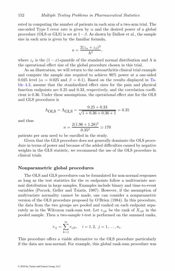
152 Multiple Testing Problems in Pharmaceutical Statistics
ested in computing the number of patients in each arm of a two-arm trial. Theone-sided Type I error rate is given by α and the desired power of a globalprocedure (OLS or GLS) is set at 1−β. As shown by Dallow et al., the samplesize in each arm is given by the familiar formula,
n =2(zα + zβ)2
Λ2,
where zx is the (1 − x)-quantile of the standard normal distribution and Λ isthe operational effect size of the global procedure chosen in this trial.
As an illustration, we will return to the osteoarthritis clinical trial exampleand compute the sample size required to achieve 90% power at a one-sided0.025 level (α = 0.025 and β = 0.1). Based on the results displayed in Ta-ble 4.3, assume that the standardized effect sizes for the pain and physicalfunction endpoints are 0.25 and 0.33, respectively, and the correlation coeffi-cient is 0.36. Under these assumptions, the operational effect size for the OLSand GLS procedures is
ΛOLS = ΛGLS =0.25 + 0.33√
1 + 0.36 + 0.36 + 1= 0.35
and thus
n =2(1.96 + 1.28)2
0.352� 170
patients per arm need to be enrolled in the study.Given that the GLS procedure does not generally dominate the OLS proce-
dure in terms of power and because of the added difficulties caused by negativeweights in the GLS statistic, we recommend the use of the OLS procedure inclinical trials.
Nonparametric global procedures
The OLS and GLS procedures can be formulated for non-normal responsesas long as the test statistics for the m endpoints follow a multivariate nor-mal distribution in large samples. Examples include binary and time-to-eventvariables (Pocock, Geller and Tsiatis, 1987). However, if the assumption ofmultivariate normality cannot be made, one can consider a nonparametricversion of the OLS procedure proposed by O’Brien (1984). In this procedure,the data from the two groups are pooled and ranked on each endpoint sepa-rately as in the Wilcoxon rank-sum test. Let rijk be the rank of Xijk in thepooled sample. Then a two-sample t-test is performed on the summed ranks,
rij =m∑
k=1
rijk , i = 1, 2, j = 1, . . . , ni.
This procedure offers a viable alternative to the OLS procedure particularlyif the data are non-normal. For example, this global rank-sum procedure was
© 2010 by Taylor and Francis Group, LLC

Analysis of Multiple Endpoints in Clinical Trials 153
used in the azithromycin study in patients with coronary artery disease (An-derson et al., 1999). The procedure was chosen to evaluate the overall effect ofthe treatment on four inflammatory markers because the change scores werenot expected to follow a normal distribution.
4.4.3 Likelihood ratio and other procedures
This section gives a review of a class of global procedures based on the like-lihood ratio (LR) principle and two other global procedures (the Lauter andFollmann procedures). This review is rather brief because these proceduresare not commonly used in clinical trial applications due to the limitationsdiscussed below.
Exact likelihood ratio procedures
It will be assumed in this section that the point null and one-sided alter-native hypotheses are given by (4.2). Kudo (1963) was the first to derive anexact one-sided LR procedure for the one-sample problem when the covariancematrix Σ is known. This procedure can be readily extended to the two-sampleproblem. Perlman (1969) extended the Kudo procedure to the case of an un-known covariance matrix but the null distribution of the resulting test statisticis not free of Σ and the procedure is biased. However, Perlman provided sharplower and upper bounds on the null distribution that are free of Σ. Wangand McDermott (1998) solved the problem of dependence on unknown Σ byderiving an LR procedure conditional on the sample covariance matrix S.
These procedures are not commonly used because they are not easy to im-plement computationally. There is, however, a more basic problem with theLR procedures that they can reject H∗
I even when the vector of mean treat-ment differences has all negative elements (Silvapulle, 1997). These proceduresare also nonmonotone in the sense that if the differences X1·k − X2·k becomemore negative the test statistic can get larger.
Perlman and Wu (2002) showed that these difficulties are caused by thepoint null hypothesis. Basically, the LR procedure compares the ratio of thelikelihood under K∗
U versus that under H∗I . The apparent nonmonotonicity of
the LR procedure results because, in some cases, as the sample outcomes movedeeper into the part of the sample space corresponding to K∗
U , their likelihoodunder K∗
U increases, but so does their likelihood under H∗I , and their ratio gets
smaller. This is not a defect of the LR procedure, but rather that of the nullhypothesis not being correctly specified. If the null hypothesis is defined as afull complement of K∗
U then the LR procedure no longer has these difficulties.However, computation of the test statistic under the complete null hypothesisand its null distribution are problematic.
Approximate LR procedures were proposed in the literature to circumventthe computational and analytical difficulties of the exact LR procedure; see,for example, Tang, Gnecco and Geller (1989) and Tamhane and Logan (2002).
© 2010 by Taylor and Francis Group, LLC
154 Multiple Testing Problems in Pharmaceutical Statistics
These procedures, although easier to apply, suffer from the same anomaliesthat the exact LR procedures suffer because of the misspecification of the nullhypothesis as a point null hypothesis.
Cohen and Sackrowitz (1998) proposed the cone-ordered monotone (COM)criterion to overcome the nonmonotonicity problem. However, their COM pro-cedure is not entirely satisfactory either since, e.g., in the bivariate case, itcan reject H∗
I if one mean difference is highly negative as long as the othermean difference is highly positive.
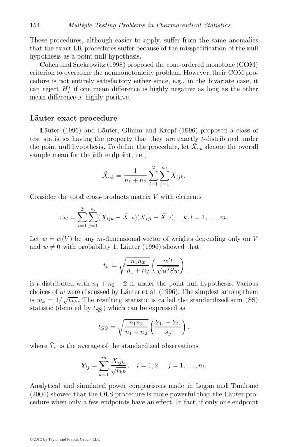
Lauter exact procedure
Lauter (1996) and Lauter, Glimm and Kropf (1996) proposed a class oftest statistics having the property that they are exactly t-distributed underthe point null hypothesis. To define the procedure, let X··k denote the overallsample mean for the kth endpoint, i.e.,
X··k =1
n1 + n2
2∑i=1
ni∑j=1
Xijk.
Consider the total cross-products matrix V with elements
vkl =2∑
i=1
ni∑j=1
(Xijk − X··k)(Xijl − X··l), k, l = 1, . . . , m.
Let w = w(V ) be any m-dimensional vector of weights depending only on Vand w �= 0 with probability 1. Lauter (1996) showed that
tw =√
n1n2
n1 + n2
(w′t√w′Sw
)is t-distributed with n1 + n2 − 2 df under the point null hypothesis. Variouschoices of w were discussed by Lauter et al. (1996). The simplest among themis wk = 1/
√vkk. The resulting statistic is called the standardized sum (SS)
statistic (denoted by tSS) which can be expressed as
tSS =√
n1n2
n1 + n2
(Y1· − Y2·
sy
),
where Yi· is the average of the standardized observations
Yij =m∑
k=1
Xijk√vkk
, i = 1, 2, j = 1, . . . , ni.
Analytical and simulated power comparisons made in Logan and Tamhane(2004) showed that the OLS procedure is more powerful than the Lauter pro-cedure when only a few endpoints have an effect. In fact, if only one endpoint
© 2010 by Taylor and Francis Group, LLC
Analysis of Multiple Endpoints in Clinical Trials 155
has an effect, which tends to infinity, the power of the Lauter procedure re-mains bounded strictly below 1, whereas the power of the OLS proceduretends to 1, as it should. Frick (1996) also noted this drawback of the Lauterprocedures but argued that such a scenario is unlikely in practice. When allendpoints have roughly equal effects, the powers of the OLS and Lauter pro-cedures are comparable.
The reason for the lack of power of the SS test statistic when only a fewendpoints have an effect is that it standardizes the data on each endpoint byits pooled total group sample standard deviation and then computes an over-all t-statistic. The pooled standard deviation overestimates the true standarddeviation since it includes the differences between the means of the treat-ment and control groups which diminishes the power of the Lauter procedure.On the other hand, the OLS statistic is the sum of t-statistics obtained bystandardizing the individual endpoints by their pooled within group samplestandard deviations.
Follmann procedure
Follmann (1996) proposed an ad-hoc procedure which is simple to apply:Reject the point null hypothesis if the two-sided Hotelling’s T 2-test is signifi-cant at the 2α-level and the average endpoint mean difference is positive,
m∑k=1
(X1·k − X2·k) > 0.
Unfortunately, the alternative for which this procedure is designed,
m∑k=1
(μ1k − μ2k) > 0,
is not very meaningful since it depends on the scaling used for the endpoints.
4.4.4 Procedures for individual endpoints
As was explained earlier in this section, global procedures are aimed at anoverall evaluation of the treatment effect. However, if the overall treatmenteffect is positive, the trial’s sponsor is likely to be interested in examiningthe treatment effect on individual endpoints/components. As pointed out inChapter 1, the LIFE trial (Dahlof et al., 2002) serves as an example of atrial in which the analysis of individual endpoints provided important in-sights into the nature of treatment benefit. This analysis revealed that theoverall treatment effect was driven mainly by one component (stroke end-point). Here we review extensions of global testing methods that can be usedto perform multiplicity-adjusted univariate inferences for individual endpointsafter a significant global result.
© 2010 by Taylor and Francis Group, LLC
156 Multiple Testing Problems in Pharmaceutical Statistics
Lehmacher, Wassmer and Reitmeir (1991) applied the closure principle tomake inferences on individual endpoints. As was explained in Section 2.3.3,this principle is a popular tool used in the construction of multiple testing pro-cedures. For example, the Holm procedure is a closed procedure for testingindividual hypotheses which is derived from the Bonferroni global procedure(see Section 4.4.2). A similar approach can be used to construct a closed testingprocedure for testing individual endpoints based on any other global proce-dure. To accomplish this, one needs to consider all possible combinations ofthe m endpoints and test each combination using an α-level global proceduresubject to the closure principle, i.e., if the procedure for any combination isnot significant then all of its subset combinations are declared nonsignificantwithout testing them. The treatment effect on an endpoint is significant atlevel α if the global procedures for all the combinations including the selectedendpoint are significant at this level.
This approach can be used with any α-level global procedure for testingdifferent intersections. Lehmacher et al. constructed a procedure for testingindividual endpoints based on the OLS and GLS procedures described in Sec-tion 4.4.2. Wang (1998) applied the Follmann procedure introduced in Sec-tion 4.4.3 as the global procedure and found the performance comparable tothe Westfall-Young resampling procedures (Section 2.8). Logan and Tamhane(2001) proposed a hybrid approach that uses a combination of global proce-dures, each one of which is powerful against a different alternative. Specifically,the Logan-Tamhane hybrid procedure consists of the Bonferroni global proce-dure based on the smallest p-value and the OLS procedure. Here the formerprocedure is powerful against alternatives where only a few endpoints havelarge effects while the latter procedure is powerful against alternatives whereall endpoints have small to modest effects. The hybrid test statistic for eachintersection hypothesis is the minimum of the p-values for the Bonferroni andOLS procedures. A bootstrap method is used to estimate the adjusted p-valuefor this complex statistic. The resulting procedure has stable and high poweragainst a range of alternatives (i.e., the procedure is robust), but is computa-tionally more intensive.
Osteoarthritis trial example
A clinical study with two endpoints (pain and physical function) was con-sidered in the osteoarthritis trial example (Section 4.4.2). The overall treat-ment effect of the two endpoints was evaluated using the OLS procedure. Theglobal procedure was significant at the one-sided 0.025 level. We will applythe closure principle to assess the treatment effect on each endpoint and seewhether the overall positive result was driven by both components or onlyone. First, we need to compute p-values for the endpoint-specific tests. FromSection 4.4.2, the t-statistics for the pain and physical function endpointsare 1.67 and 2.18, respectively, with n1 + n2 − 2 = 172 df. The one-sidedp-values associated with the t-statistics are 0.0486 and 0.0152 applying the
© 2010 by Taylor and Francis Group, LLC

Analysis of Multiple Endpoints in Clinical Trials 157
Logan-Tamhane formula for degrees of freedom. Using the closure principle,the multiplicity adjusted p-value for each endpoint is the larger of the p-valuefor the OLS procedure and the p-value for the endpoint-specific t-test. Thetreatment’s effect on the pain endpoint is not significant at the one-sided0.025 level (p = 0.0486) whereas the effect on the other endpoint is significant(p = 0.0152). It is worth remembering that it is possible for endpoint-specifictests to be non-significant even if the global procedure is highly significant.
4.5 All-or-none procedures
As was explained in Section 4.2.3, the goal of demonstrating the efficacy ofthe treatment on all endpoints requires an all-or-none or IU procedure (Berger,1982) of the union of individual hypotheses, Hi. The all-or-none procedure hasthe following form:
Reject all hypotheses if tmin = min1≤i≤m
ti ≥ tα(ν),
where tα(ν) is the (1 − α)-quantile of the t-distribution with ν = n1 + n2 − 2df. This procedure is popularly known as the min test (Laska and Meisner,1989).
Since this procedure does not use a multiplicity adjustment (each hypoth-esis Hi is tested at level α), it may appear at first that it must be highlypowerful as a test of the global hypothesis HU . In reality, the min test is veryconservative because of the requirement that all hypotheses must be rejectedat level α. The conservatism results from the least favorable configuration ofthe min test which can be shown to be of the following form:
• No treatment effect for any one endpoint (δi = 0 for some i).
• Infinitely large treatment effects for all other endpoints (δj → ∞ forj �= i).
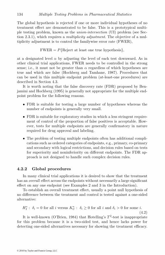
This configuration leads to marginal α-level t-tests.Figure 4.2, based on Offen et al. (2007), will help the reader appreciate how
conservative the min test can be. This figure gives the multipliers to calculatethe sample size required to guarantee 80% power for the min test if the basesample size guarantees 80% power for each endpoint. The calculation was doneunder the assumption of equicorrelated endpoints and a common standardizedeffect size for all endpoints. As can be seen from the table, the multiplierincreases as the number of endpoints increases and the assumed commoncorrelation between them decreases. Consider, for example, the clinical trial inpatients with Alzheimer’s disease described by Offen and Helterbrand (2003).It is commonly required that a new treatment should demonstrate a significant
© 2010 by Taylor and Francis Group, LLC

158 Multiple Testing Problems in Pharmaceutical Statistics
0.0 0.2 0.4 0.6 0.8 1.0
1.0
1.2
1.4
1.6
1.8
2.0
Correlation coefficient
Mul
tiplie
r
FIGURE 4.2: Sample size multipliers for the min test for two endpoints(solid curve) and four endpoints (dashed curve) as a function of the commoncorrelation in all-or-none testing problems. Multiplier equals 1 for a singleendpoint.
effect on at least two endpoints, e.g., a cognition endpoint (Alzheimer’s DiseaseAssessment Scale-Cognitive Subpart) and a clinical global scale (Clinician’sInterview-Based Impression of Change). The correlation between these twoendpoints is usually around 0.2 and thus the sample size multiplier is 1.29which corresponds to almost a 30% increase in the sample size. In other cases,e.g., when four weakly correlated endpoints are considered, the multiplieris 1.58 meaning that the sample size needs to be increased by almost 60%compared to the single-endpoint case.
It is important to note that the least favorable configuration for the mintest is clinically not plausible. The global hypothesis HU permits configura-tions with infinitely large positive effects on some endpoints and negative ef-fects on others. However, it is uncommon for treatments to have substantiallydifferent effects on the endpoints. This has led researchers to put restrictionson the global hypothesis in order to develop more powerful versions of the mintest.
Hochberg and Mosier (2001) suggested restricting HU to the negativequadrant,
m⋂k=1
(δk ≤ 0),
© 2010 by Taylor and Francis Group, LLC
Analysis of Multiple Endpoints in Clinical Trials 159
in which case the least favorable configuration is the overall null configuration,δ1 = . . . = δm = 0. Chuang-Stein et al. (2007) restricted the hypothesis to thesubset of the global hypothesis which satisfies
m⋂k=1
(−εk ≤ δk ≤ εk),
where the thresholds εk, k = 1, . . . , m, are prespecified based on clinical con-siderations. A similar approach, but based on estimated mean differences,X1·k − X2·k, was proposed by Snapinn (1987). Cappizi and Zhang (1996) sug-gested another alternative to the min test which requires that the treatmentbe shown effective at a more stringent significance level α1 on say m1 < mendpoints and at a less stringent significance level α2 > α1 on the remainingm2 = m−m1 endpoints. For m = 2, they suggested this rule for m1 = m2 = 1,α1 = 0.05 and α2 = 0.10 or 0.20. However, as pointed out by Neuhauser,Steinijans and Bretz (1999), this rule does not control the FWER at α = 0.05.
Another approach to this formulation adopts a modified definition of theerror rate to improve the power of the min test in clinical trials with severalendpoints. Chuang-Stein et al. (2007) considered an error rate definition basedon the average Type I error rate over the null space and developed a procedurethat adjusts significance levels for the individual endpoints to control theaverage Type I error rate at a prespecified level.
This is a relatively new research area and further work is required to assessthe utility of the methods described in this section and their applicability.
4.6 Superiority-noninferiority procedures
There are many situations in which the requirement that the treatment besuperior to the control on all endpoints (all-or-none procedures in Section 4.5)is often too strong and the requirement that the treatment be superior to thecontrol on at least one endpoint (at-least-one procedures in Section 4.3) istoo weak. The superiority-noninferiority approach discussed in this sectionstrengthens the latter requirement by augmenting it with the additional re-quirement that the treatment is not inferior to the control on all other end-points.
Consider a clinical trial with m endpoints and suppose that its objectiveis to demonstrate the treatment is superior to the control on at least oneendpoint and noninferior to the control on all other endpoints. Note that ifsuperiority is established for both endpoints, the second part of this require-ment (noninferiority) becomes redundant. This formulation of the superiority-noninferiority testing problem was considered by Bloch, Lai and Tubert-Bitter(2001) and Tamhane and Logan (2004). The null and alternative hypotheses
© 2010 by Taylor and Francis Group, LLC

160 Multiple Testing Problems in Pharmaceutical Statistics
for the superiority-noninferiority problem are defined in Section 4.2.4:
H(SN)U = H
(S)I ∪ H
(N)U versus K
(SN)I = K
(S)U ∩ K
(N)I .
The trial’s outcome is declared positive if there is evidence of superior efficacyfor at least one endpoint (K(S)
U ) and noninferior efficacy for all endpoints(K(N)
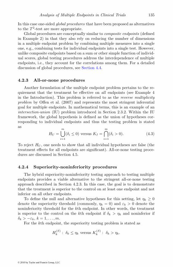
I ).As an illustration, consider a clinical trial with two endpoints. The region
corresponding to the alternative hypothesis K(SN)I with ε1 = 5, ε2 = 7, η1 = 3
and η2 = 4 is shown in Figure 4.3.
−10 −5 0 5 10
−10
−5
05
10
δ1
δ 2 ε1
ε2
η1
η2
FIGURE 4.3: Region in the parameter space corresponding to the alternativehypothesis (shaded area) in a superiority-noninferiority testing problem withtwo endpoints.
Tamhane-Logan superiority-noninferiority procedure
Denote the t-statistics for superiority and noninferiority for the kth end-point by
t(S)k =
X1·k − X2·k − ηk
sk
√1/n1 + 1/n2
, t(N)k =
X1·k − X2·k + εk
sk
√1/n1 + 1/n2
.
Tamhane and Logan (2004) used the UI statistic
t(S)max = max(t(S)
1 , . . . , t(S)m )
© 2010 by Taylor and Francis Group, LLC

Analysis of Multiple Endpoints in Clinical Trials 161
for testing the superiority null hypothesis H(S)I and the IU statistic
t(N)min = min(t(N)
1 , . . . , t(N)m )
for testing the noninferiority null hypothesis H(N)U . They proposed the follow-
ing procedure of the global superiority-noninferiority hypothesis:
Reject H(SN)U if t(S)
max ≥ c(S) and t(N)min ≥ c(N),
where the critical values c(S) and c(N) are chosen so that the procedure haslevel α. Bloch et al. (2001) used the Hotelling T 2-statistic for testing superi-ority in place of t
(S)max; however, as noted before, the T 2-statistic is not very
powerful against one-sided superiority alternative. Perlman and Wu (2004)used Perlman’s one-sided LR statistic instead of the T 2-statistic.
According to the intersection-union testing principle, the superiority andnoninferiority tests must be of level α. Conservative values for c(S) and c(N)
can be chosen to be the (1−α/m)- and (1−α)-quantiles of the t-distribution,respectively, with ν = n1 +n2−2 df. The exact value of c(S) involves the gen-eralized multivariate t distribution and thus, as was explained in Section 4.3.2,is difficult to evaluate. Also, a sharper critical constant c(S) can be evaluatedby conditioning on the event that the noninferiority test is passed by all end-points. However, the resulting value of c(S) needs to be evaluated by usingbootstrap; see Bloch et al. (2001) and Tamhane and Logan (2004). Rohmelet al. (2006) objected to this conditioning arguing that it causes significanceof the superiority test to be influenced by changes in the noninferiority mar-gin for which there is no clinical justification. However, Logan and Tamhane(2008) showed that passing the noninferiority test at a more stringent marginadds more credence to the alternative hypothesis K
(S)U that the treatment
is superior on at least one endpoint, and therefore it is retained more eas-ily. If H
(SN)U = H
(S)I ∪ H
(N)U is rejected then it is of interest to know which
endpoints demonstrate superiority of the treatment over the control. Loganand Tamhane (2008) gave a closed procedure for this purpose which controlsFWER for the family of H
(SN)U as well as the endpoint-specific superiority
null hypotheses H(S)k . This closed procedure can be implemented in m + 1
steps.
Alzheimer’s disease trial example
The Alzheimer’s disease example from Section 4.5 will be used to illus-trate key properties of the Tamhane-Logan superiority-noninferiority proce-dure. Table 4.4 displays results of a 24-week study in patients with Alzheimer’sdisease that tested the efficacy and safety of an experimental treatment com-pared to placebo. The efficacy profile of the treatment was evaluated usingtwo co-primary endpoints, Alzheimer’s Disease Assessment Scale-Cognitive
© 2010 by Taylor and Francis Group, LLC

162 Multiple Testing Problems in Pharmaceutical Statistics
TABLE 4.4: Summary of the results ofAlzheimer’s disease trial (SD, standard deviation).
Endpoint Summary Treatment Placebostatistic n = 167 n = 161
ADAS-Cog Mean 0.5 2.5Pooled SD 7.4 7.4
CIBIC-Plus Mean 4.2 4.4Pooled SD 1.1 1.1
Subpart (ADAS-Cog) and Clinician’s Interview-Based Impression of Change(CIBIC-Plus).
Suppose that the superiority margins are set at 0 and the noninferioritymargins for the ADAS-Cog and CIBIC-Plus endpoints at 0.8 and 0.1, re-spectively. Based on this information, the superiority and noninferiority teststatistics are given by[
t(S)1
t(S)2
]=[
2.451.65
],
[t(N)1
t(N)2
]=[
3.432.47
].
Further, assuming a one-sided α = 0.025, the critical values of theTamhane-Logan procedure are
c(S) = t0.0125(326) = 2.25 and c(N) = t0.025(326) = 1.97.
The rejection region of the superiority-noninferiority procedure is shown inFigure 4.4. The superiority and noninferiority test statistics are in their cor-responding rejection regions, i.e.,
max(t(S)1 , t
(S)2 ) ≥ 2.25 and min(t(N)
1 , t(N)2 ) ≥ 1.97,
and thus the procedure rejects the global superiority-noninferiority hypothe-sis. To determine which individual endpoints demonstrate superiority of thetreatment, t
(S)1 and t
(S)2 are compared with t0.025(326) = 1.97. Since only t
(S)1
exceeds this critical constant, superiority is demonstrated only on ADAS-Cog;noninferiority is demonstrated on CIBIC-Plus.
Note that the Tamhane-Logan procedure is monotone in the sense that, ifa certain set of test statistics leads to the rejection of the global superiority-noninferiority hypothesis, the hypothesis will be rejected for any set of moreextreme test statistics.
It is instructive to compare the Tamhane-Logan superiority-noninferiorityprocedure to the min test used in the all-or-none testing problem described inSection 4.5. The min test rejects the global superiority hypothesis if
min(t(S)1 , t
(S)2 ) ≥ t0.025(326) = 1.97.
© 2010 by Taylor and Francis Group, LLC

Analysis of Multiple Endpoints in Clinical Trials 163
0 1 2 3 4
01
23
4
t1
t 2
0 1 2 3 4
01
23
4t1
t 2
FIGURE 4.4: Left panel: Rejection region of the superiority componentof the Tamhane-Logan procedure (shaded area) and superiority test statis-tics (dot). Right panel: Rejection region of the noninferiority component ofthe Tamhane-Logan procedure (shaded area) and noninferiority test statistics(dot).
The rejection region of the min test is displayed in Figure 4.5. It is clear thatthe global superiority hypothesis cannot be rejected since the treatment effectfor CIBIC-Plus is not significant at the one-sided 0.025 level (t(S)
2 < 1.97).This serves as an illustration of the fact that the all-or-none testing approachis based on more stringent criteria compared to the superiority-noninferioritytesting approach.
4.7 Software implementation
This section briefly describes software implementation of the multiple andglobal procedures discussed in this chapter. The following SAS programs wereused in the examples included in this chapter. The programs can be down-loaded from the book’s Web site (http://www.multxpert.com).
• Program 2.1 can be used to implement at-least-one procedures for iden-tifying the treatment effect on individual endpoints described in Sec-tion 4.3, including the Bonferroni, fixed-sequence and fallback proce-
© 2010 by Taylor and Francis Group, LLC

164 Multiple Testing Problems in Pharmaceutical Statistics
0 1 2 3 4
01
23
4
t1
t 2
FIGURE 4.5: Rejection region of the min test (shaded area) and superioritytest statistics (dot).
dures (note that this program also implements other p-value-based pro-cedures introduced in Section 2.6). Software implementation of the para-metric fallback and 4A procedures is not currently available. Criticalvalues for these procedures are tabulated in Huque and Alosh (2008)and Li and Mehrotra (2008), respectively.
• Program 4.1 implements the OLS and GLS procedures in the os-teoarthritis trial example introduced in Section 4.4.2. Program 4.2 per-forms sample size calculations for the OLS and GLS procedures in thisclinical trial example.
• Program 4.3 implements the Tamhane-Logan superiority-noninferiorityprocedure in the Alzheimer’s disease trial example (Section 4.6).
Acknowledgements
Ajit C. Tamhane’s research was supported by grants from the NationalHeart, Lung and Blood Institute.
© 2010 by Taylor and Francis Group, LLC


![[XLS] · Web viewSUNITA BARMAN C000060491 SMITA JAIN B-19,SHAKTI NAGAR PO GAVERA PROJECT, KORBA CHHATISGARH RAVI KUMAR SATRANJ RELIABLE FINANCIAL CONSULTANTS VIJAY KESHEO TAMHANE](https://img.pdfslide.us/doc/110x75/5ac87bcd7f8b9aa3298c2618/xls-viewsunita-barman-c000060491-smita-jain-b-19shakti-nagar-po-gavera-project.jpg)