Embed Size (px)
Citation preview

206
CHAPTER 4
THE AVERAGE MODEL OF THE SYMMETRICAL AND SYMMETRICAL
MULTIPLE-STAR IPM MACHINES
4.1 Introduction
For many studies the simplified model of a machine is needed. The simplified models can
be used for designing the drives, steady state analysis and decoupling of the models [120]. This
chapter starts with the modelling of symmetrical and asymmetrical triple-star nine-phase machines
using the Fourier series. After generating the general equations for turn functions of the machines
phases, the general form of the Fourier series of the winding functions are derived. The Fourier
series of the airgap function of the machines are also derived in this chapter and using them the
general form of the Fourier series of different inductances of the machines stators are derived. In
the next section by neglecting the inductances with the higher order harmonics the simplified
inductances are presented. The simplified inductances are then transformed to the rotor reference
frame and the general model of the machines is generated. To verify the machines model, they are
simulated using the MATLAB Simulink and the simulation results are presented. The general
model of the machines is decoupled to remove the coupling terms between different machines and
the decoupled models for symmetrical and asymmetrical machines are presented. In the final
sections of this chapter an asymmetrical double-star six-phase IPM is also modelled using Fourier
series of the machine parameters [83]. The model is generated and transformed to the rotor

207
reference frame and finally the model is decoupled to remove the couplings between the two sets
of the three phase machines. The major contribution of this chapter is generating decoupled models
and corresponding transformation matrixes for triple-star nine-phase IPM machines (symmetrical
and asymmetrical connections) that can be used for designing controllers for triple-star machines
without facing the complexities raised by the coupling terms between different sets of the three
phase machines.
A1+
A1+
B3-
B3-A2+
A2+
A1+
A1+
B3-
B3-A2+
A2+
A1- A1-
B3+B3+
A2-A2-
A1- A1-
B3+B3+
A2-A2-
C1-
C1-A3+
A3+
C2-C2-
C1-
C1-
A3+
A3+
C2-C2-
C1+
C1+A3-
A3-
C2+
C2+
C1+C1+
A3-
A3-C2+
C2+
B1+B1+
C3- C3-
B2+B2+
B1+B1+
C3-
B2+B2+
B2-
B2-
C3+B1-
C3+B1-
B2-
B2-
C3+
C3+
B1-
B1-
1 23
4
5
6
7
8
9
10
11
12
13
14
1516
1718192021
22
23
24
25
26
27
28
29
30
31
32
33
3435
36
C3-
Figure 4.1: The clock diagram of the symmetrical triple-star machine.
4.2 Modelling the Stator Inductances of Triple-Star Machines

208
In this section the stator inductances of both symmetrical and asymmetrical triple-star IPM
machines are modeled using the Fourier series of the machine parameters such as the winding
functions and airgap functions.
50 100 150 200 250 300 350 400
50 100 150 200 250 300 350 400
50 100 150 200 250 300 350 400
NA1
NB1
NC1
Ɵ (Degree)
50
50
-50
Figure 4.2: The turn functions of the machine 1 phases (symmetrical).
50 100 150 200 250 300 350 400
50 100 150 200 250 300 350 400
50 100 150 200 250 300 350 400
NA2
NB2
NC2
Ɵ (Degree)
50
50
-50
Figure 4.3: The turn functions of the machine 2 phases (symmetrical).
50 100 150 200 250 300 350 400
50 100 150 200 250 300 350 400
50 100 150 200 250 300 350 400
Ɵ (Degree)
50
50
-50
NA3
NB3
NC3
Figure 4.4: The turn functions of the machine 3 phases (symmetrical).

209
Unlike the coupled modelling, there will be some simplifying assumptions made to have a
simpler model. For example, in this modelling method, the higher frequency order components of
the winding functions and airgap functions are neglected. The modelling can start from the clock
diagram and turn functions of the machine. The clock diagram and the turn functions of the
symmetrical machine (shown in Figure 4.1) are repeated here in Figures 4.2 to 4.4. Similarly, for
the asymmetrical machine the turn functions can be generated using the clock diagram, the clock
diagram of the asymmetrical machine is shown in the Figure 4.5.
A1+
A1+
B3-
B3-
A2+
A2+
A1+
A1+
B3-
B3-
A2+
A2+
A1- A1-
B3+B3+
A2-A2-
A1-
B3+B3+
A2- A2-
C1-
C1-
A3+
A3+
C2-
C2-
C1-
C1-
A3+
A3+
C2-
C2-C1+
C1+
A3-A3-
C2+
C2+
C1+C1+
A3-A3-
C2+
C2+
B1+B1+
C3-C3-
B2+
B1+B1+
C3-C3-
B2+B2+
B2-
B2-C3+
B1-
C3+
B1-
B2-
B2-
C3+
C3+B1-
B1-
1 23
4
5
6
7
8
9
10
11
12
13
14
1516
1718192021
22
23
24
25
26
27
28
29
30
31
32
33
3435
36
B2+
A1-
Figure 4.5: The clock diagram of the asymmetrical triple-star machine.
Using the new clock diagram the turn functions can be generated as Figures 4.6 to 4.8.

210
50 100 150 200 250 300 350 400
50 100 150 200 250 300 350 400
50 100 150 200 250 300 350 400
NA1
Ɵ (Degree)
50
50
-50
NB1
NC1
Figure 4.6: The turn functions of the machine 1 phases (asymmetrical).
50 100 150 200 250 300 350 400
50 100 150 200 250 300 350 400
50 100 150 200 250 300 350 400
NA2
Ɵ (Degree)
50
50
50
NB2
NC2
Figure 4.7: The turn functions of the machine 2 phases (asymmetrical).
50 100 150 200 250 300 350 400
50 100 150 200 250 300 350 400
50 100 150 200 250 300 350 400
NA3
Ɵ (Degree)
50
50
50
NB3
NC3
Figure 4.8: The turn functions of the machine 3 phases (asymmetrical).
Based on the above figures the general form of Fourier series of the turn function can be
generated as:

211
)(7sin)(5sin
)(3sin)sin(
75
310
kk
kkx
kdNkdN
kdNkdNNn
n
NN
NNicbax x
nx
iii
4,
2,
93,2,1,,, 0
(4.1)
Where: ‘ kd ’ equals to 1 and 2 for the symmetrical and asymmetrical machines
respectively. Also, for each phase that is placed in slot number ‘S’ the ‘k’ can be defined as:
1 Sk
(4.2)
Also, based on Figure 3.6, the Fourier series of the inverse airgap function can be presented
as [152]:
)(14cos)(10cos
)(6cos)(2cos),(
43
210
1
rr
rrr
aa
aaag
(4.3)
Where, a0, a1, a3, a4 are the Fourier series amplitudes for the inverse air gap function and
can be defined as:
,0 aa ba 1,
32
ba ,
53
ba ,
74
ba
bb gga
11
2
1,
ab ggb
11
2
1
(4.4)
Using the equations (4.1) and (4.3) the winding function of each phase can be calculated
as [74]:

212
2
0
2
0
),(
1
),(
)(
)()(
dg
dg
n
nN
r
r
w
ww
(4.5)
The different parts of the equation (4.5) can be expressed as:
2
0
0
43
2102
0
2)(14cos)(10cos
)(6cos)(2cos
),(
1ad
aa
aaad
g rr
rr
r
(4.6)
2
0
0000
2
0
432107
432105
432103
432101
432100
2
0 43210
753102
0
2
)(14cos)(10cos)(6cos)(2cos)(7sin
)(14cos)(10cos)(6cos)(2cos)(5sin
)(14cos)(10cos)(6cos)(2cos)(3sin
)(14cos)(10cos)(6cos)(2cos)sin(
)(14cos)(10cos)(6cos)(2cos
)(14cos)(10cos)(6cos)(2cos
)(7sin)(5sin)(3sin)sin(
),(
)(
aNdaN
d
aaaaakdN
aaaaakdN
aaaaakdN
aaaaakdN
aaaaaN
daaaaa
kdNkdNkdNkdNNd
g
n
rrrrk
rrrrk
rrrrk
rrrrk
rrrr
rrrr
kkkk
r
w
(4.7)
Therefore, equations (4.6) and (4.7) result in:
0
0
00
2
0
2
0
2
2
),(
1
),(
)(
Na
aN
dg
dg
n
r
r
w
(4.8)
Using the above equations, the general form of the winding functions of the machines can
be expressed as:
)(7sin)(5sin)(3sin)sin(
)(7sin)(5sin)(3sin)sin()(
7531
075310
kkkk
kkkkw
kdNkdNkdNkdN
NkdNkdNkdNkdNNN
(4.9)
Now the general form of the self and mutual inductances (between phases ‘j’ and ‘i’) of
the machines phases can be generated as:

213
2
0
75310
7531
43210
2
0
)(7sin)(5sin)(3sin)sin(
)(7sin)(5sin)(3sin)sin(
)(14cos)(10cos)(6cos)(2cos
)()(),(
1
d
dkNdkNdkNdkNN
dkNdkNdkNdkN
aaaaa
rl
dNng
rlL
kikikiki
kjkjkjkj
rrrr
o
ij
r
oji
(4.10)
The equation (4.10) is equal to:
2
0
77
7573
7170
57
5553
5150
37
3533
3130
17
1513
1110
43210
2
0
)(7sin)(7sin
)(5sin)(7sin)(3sin)(7sin
)sin()(7sin)(7sin
)(7sin)(5sin
)(5sin)(5sin)(3sin)(5sin
)sin()(5sin)(5sin
)(7sin)(3sin
)(5sin)(3sin)(3sin)(3sin
)sin()(3sin)(3sin
)(7sin)sin(
)(5sin)sin()(3sin)sin(
)sin()sin()sin(
)(14cos)(10cos)(6cos)(2cos
)()(),(
1
d
dkdkNN
dkdkNNdkdkNN
dkdkNNdkNN
dkdkNN
dkdkNNdkdkNN
dkdkNNdkNN
dkdkNN
dkdkNNdkdkNN
dkdkNNdkNN
dkdkNN
dkdkNNdkdkNN
dkdkNNdkNN
aaaaa
rl
dNng
rlL
kikj
kikjkikj
kikjkj
kikj
kikjkikj
kikjkj
kikj
kikjkikj
kikjkj
kikj
kikjkikj
kikjkj
rrrr
o
ij
r
oji
(4.11)
The non-zero terms are:

214
2
0
7770
5550
3330
1110
43210
2
0
)(7sin)(7sin)(7sin
)(5sin)(5sin)(5sin
)(3sin)(3sin)(3sin
)sin()sin()sin(
)(14cos)(10cos)(6cos)(2cos
)()()(),(
1
d
dkdkNNdkNN
dkdkNNdkNN
dkdkNNdkNN
dkdkNNdkNN
aaaaa
rl
dNng
rlL
kikjkj
kikjkj
kikjkj
kikjkj
rrrr
o
ij
r
oji
(4.12)
The equation (4.12) is equal to:
2
0
2
770
2
550
2
330
2
110
43210
2
0
7cos27cos2
)(7sin
5cos25cos2
)(5sin
3cos23cos2
3sin
cos2cos2
sin
)(14cos)(10cos)(6cos)(2cos
)()(),(
1
d
kkdkkdN
dkNN
kkdkkdN
dkNN
kkdkkdN
dkNN
kkdkkdN
dkNN
aaaaa
rl
dNng
rlL
jikijkj
jikijkkj
jikijkkj
jikijkkj
rrrr
o
ij
r
oji
(4.13)
And the term with non-zero averages are:

215
2
02
74
2
53
2
32
2
11
2
7
2
5
2
3
2
10
2
0
)(14cos27cos2
)(10cos25cos2
)(6cos23cos2
)(2cos2cos2
7cos2
5cos2
3cos2
cos2
)()()(),(
1
d
kkdN
akkdN
a
kkdN
akkdN
a
kkdN
kkdN
kkdN
kkdN
a
rl
dNng
rlL
rijkrijk
rijkrijk
jikjijikjik
o
ij
r
oji
(4.14)
The last equation is equal to:
2
0
2
74
2
53
2
32
2
11
2
7
2
5
2
3
2
1
0
2
0
714cos71428cos4
510cos51020cos4
36cos3612cos4
2cos24cos4
7cos2
5cos2
3cos2
cos2
)()()(),(
1
d
kkdkkdN
a
kkdkkdN
a
kkdkkdN
a
kkdkkdN
a
kkdN
kkdN
kkdN
kkdN
a
rl
dNng
rlL
ijkrijkr
ijkrijkr
ijkrijkr
ijkrijkr
jikjik
jikjik
o
ij
r
oji
(4.15)
And finally the stator inductances can be expressed as:

216
ijkrijkr
ijkrijkr
jikjik
jikjik
o
ij
r
oji
kkdN
akkdN
a
kkdN
akkdN
a
kkdN
kkdN
kkdN
kkdN
a
rl
dNng
rlL
714cos4
510cos4
36cos4
2cos4
7cos2
5cos2
3cos2
cos2
2
)()()(),(
1
2
74
2
53
2
32
2
11
2
7
2
5
2
3
2
1
0
2
0
(4.16)
Where ‘ ik ’ and ‘ jk ’ are:
1, NumberSlotingCorrespondk ji (4.17)
The machines inductances have different harmonics including DC, second, sixth, tenth and
fourteenth order. Neglecting the harmonics with frequencies higher than two, the general equation
for the inductances can be derived as:
ijkrjiko
ij
r
oji
kkdN
akkdN
arl
dNng
rlL
2cos4
cos2
2
)()(),(
1
2
11
2
10
2
0
(4.18)
4.3 Transformation of the Inductances to the Rotor Reference Frame
The inductances of the machines can be arranged inside a 9×9 matrix and be transformed
to the rotor reference frame using the transformation presented in section 3.4.

217
0303303303
3033333
3033333
0203302302
2033232
2033232
0103301301
1033131
1033131
0203302302
2033232
2033232
0202202202
2022222
2022222
0102201201
1022121
1022121
0103301301
1033131
1033131
0102201201
1022121
1022121
0101101101
1011111
1011111
33
33
33
22
22
22
11
11
11
333333232323131313
333333232323131313
333333232323131313
323232222222121212
323232222222121212
323232222222121212
313131212121111111
313131212121111111
313131212121111111
333
333
222
222
111
111
1
1000000
1000000
1000000
0001000
0001000
0001000
0000001
0000001
0000001
2
1
2
1
2
1000000
000000
000000
0002
1
2
1
2
1000
000000
000000
0000002
1
2
1
2
1
000000
000000
3
2
LLL
LLL
LLL
LLL
LLL
LLL
LLL
LLL
LLL
LLL
LLL
LLL
LLL
LLL
LLL
LLL
LLL
LLL
LLL
LLL
LLL
LLL
LLL
LLL
LLL
LLL
LLL
SC
SC
SC
SC
SC
SC
SC
SC
SC
LLLLLLLLL
LLLLLLLLL
LLLLLLLLL
LLLLLLLLL
LLLLLLLLL
LLLLLLLLL
LLLLLLLLL
LLLLLLLLL
LLLLLLLLL
SSS
CCC
SSS
CCC
SSS
CCC
TLT
dq
dddqd
qdqqq
dq
dddqd
qdqqq
dq
dddqd
qdqqq
dq
dddqd
qdqqq
dq
dddqd
qdqqq
dq
dddqd
qdqqq
dq
dddqd
qdqqq
dq
dddqd
qdqqq
dq
dddqd
qdqqq
rr
rr
rr
rr
rr
rr
rr
rr
rr
ccbcacccbcacccbcac
cbbbabcbbbabcbbbab
cabaaacabaaacabaaa
ccbcacccbcacccbcac
cbbbabcbbbabcbbbab
cabaaacabaaacabaaa
ccbcacccbcacccbcac
cbbbabcbbbabcbbbab
cabaaacabaaacabaaa
rrr
rrr
rrr
rrr
rrr
rrr
rssr
(4.19)
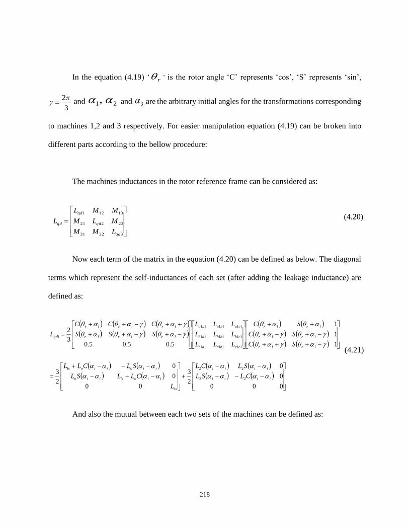
218
In the equation (4.19) ‘ r ’ is the rotor angle ‘C’ represents ‘cos’, ‘S’ represents ‘sin’,
3
2 and 21, and 3 are the arbitrary initial angles for the transformations corresponding
to machines 1,2 and 3 respectively. For easier manipulation equation (4.19) can be broken into
different parts according to the bellow procedure:
The machines inductances in the rotor reference frame can be considered as:
33231
23221
13121
qd
qd
qd
qd
LMM
MLM
MML
L
(4.20)
Now each term of the matrix in the equation (4.20) can be defined as below. The diagonal
terms which represent the self-inductances of each set (after adding the leakage inductance) are
defined as:
000
0
0
2
3
00
0
0
2
3
1
1
1
5.05.05.03
2
22
22
111111
111111
111111
iiii
iiii
ls
iiolsiio
iioiiols
irir
irir
irir
ccbcac
cbbbab
cabaaa
iririr
iririr
qdi
CLSL
SLCL
L
CLLSL
SLCLL
SC
SC
SC
LLL
LLL
LLL
SSS
CCC
L
(4.21)
And also the mutual between each two sets of the machines can be defined as:

219
000
0)2()2(
0)2()2(
2
3
000
0)()(
0)()(
2
3
1
1
1
5.05.05.03
2
1212
1212
313131
313131
313131
kjkkjk
kjkkjk
kjkokjko
kjkokjko
jrjr
jrjr
jrjr
ccbcac
cbbbab
cabaaa
krkrkr
krkrkr
kjqd
djkCLdjkSL
djkSLdjkCL
djkCLdjkSL
djkSLdjkCL
SC
SC
SC
LLL
LLL
LLL
SSS
CCC
M
(4.22)
Where:
0
2
10 arlNL o 2
12
12
arlNL o
(4.23)
The non-diagonal terms of the equation (4.21) are equal to zero. To remove coupling
between the different axis of the machines, the non-diagonal terms of the equation (4.22) should
be equal to zero. By setting them equal to zero the proper initial angles can be calculated as
equations (4.24) and (4.25).
kjkkjk djkdjkS )(0)(
(4.24)
11 )2(0)2( kjkkjk djkdjkS (4.25)
For different combinations of ‘k’ and ‘j’ the initial angles are calculated and given in Table
4.1. This table represents the proper initial values and the coefficients to remove the couplings
between ‘q’ and ‘d’.

220
Table 4.1 The initial angle for the transformation d1 and dk1 for different machines.
1kd 1d
1 2 3
Symmetrical 4 2 0
9
2
9
4
Asymmetrical 1 1 0
9
9
2
By substituting the values of equation (4.23) in the equations (4.21) and (4.22) and
selecting the initial values of Table 4.1 the inductance matrixes change to:
ls
dd
ls
ls
ls
qd
L
L
L
L
LLL
LLL
L
00
00
00
00
00
00
2
311
11
20
20
1
(4.26)
ls
dd
ls
ls
ls
qd
L
L
L
L
LLL
LLL
L
00
00
00
00
00
00
2
322
22
20
20
2
(4.27)
ls
dd
ls
ls
ls
qd
L
L
L
L
LLL
LLL
L
00
00
00
00
00
00
2
333
33
20
20
3
(4.28)
000
00
00
000
00
00
2
331
31
20
20
13 dd
qd L
L
LL
LL
M
(4.29)

221
000
00
00
000
00
00
2
313
13
20
20
31 dd
qd L
L
LL
LL
M
(4.30)
000
00
00
000
00
00
2
321
21
20
20
12 dd
qd L
L
LL
LL
M
(4.31)
000
00
00
000
00
00
2
312
12
20
20
21 dd
qd L
L
LL
LL
M
(4.32)
000
00
00
000
00
00
2
332
32
20
20
23 dd
qd L
L
LL
LL
M
(4.33)
000
00
00
000
00
00
2
323
23
20
20
32 dd
qd L
L
LL
LL
M
(4.34)
Now using equations (4.26) to (4.34) the machines inductances in the rotor reference frame
can be presented as equation (4.35). Unlike the models that were generated in the Sections 3.3 and
3.4, in this matrix the mutual inductances between the d and q axis are zero. This fact is due to
ignoring the higher order harmonics of the winding functions and airgap function. By substituting
the matrix of equation (4.35) in to the model of Section 3.2 the machines model can be expressed
as equation (4.36).

222
ls
lsdddddd
lsqqqqqq
ls
ddlsdddd
qqlsqqqq
ls
ddddlsdd
qqqqlsqq
qd
L
LLLL
LLLL
L
LLLL
LLLL
L
LLLL
LLLL
L
00000000
000000
000000
00000000
000000
000000
00000000
000000
000000
332313
332313
322212
322212
312111
312111
(4.35)
33
32231133333
2231133333
22
233211122222
3321122222
11
13312211111
3312211111
olso
pmddddddddlsddd
qqqqqqqlsqqq
olso
pmddddqddddlsddd
qqqqqqqlsqqq
olso
pmddddddddlsddd
qqqqqqqlsqqq
iL
iLiLiLL
iLiLiLL
iL
iLiLiLL
iLiLiLL
iL
iLiLiLL
iLiLiLL
(4.36)
By substituting the flux linkages of equation (4.36) in to the voltage equations (3.59) to
(3.61) the machines voltages in the rotor reference frame can be expressed as equation (4.37). The
equivalent circuits of the q and d axis and also zero sequence are shown in Figures 4.9 to 4.11.

223
0
0
0
0
0
0
00000000
000000
000000
00000000
000000
000000
00000000
000000
000000
0
0
0
0
0
0
00000000
000000
000000
00000000
000000
000000
00000000
000000
000000
000000000
001000000
010000000
000000000
000001000
000010000
000000000
000000001
000000010
1
1
1
3
3
3
2
2
2
1
1
1
332313
332313
322212
322212
312111
312111
1
1
1
3
3
3
2
2
2
1
1
1
332313
332313
322212
322212
312111
312111
3
3
3
2
2
2
1
1
1
3
3
3
2
2
2
1
1
1
pmd
pmd
pmd
o
d
q
o
d
q
o
d
q
ls
lsdddddd
lsqqqqqq
ls
ddlsdddd
qqlsqqqq
ls
ddddlsdd
qqqqlsqq
pmd
pmd
pmd
o
d
q
o
d
q
o
d
q
ls
dddddd
qqqqqq
ls
dddddd
qqqqqq
ls
dddddd
qqqqqq
r
o
d
q
o
d
q
o
d
q
se
o
d
q
o
d
q
o
d
q
i
i
i
i
i
i
i
i
i
L
LLLL
LLLL
L
LLLL
LLLL
L
LLLL
LLLL
p
i
i
i
i
i
i
i
i
i
L
LLL
LLL
L
LLL
LLL
L
LLL
LLL
i
i
i
i
i
i
i
i
i
r
V
V
V
V
V
V
V
V
V
(4.37)

224
rse
Lq1q1
Lls
1dr
1qV
1qi rseLls2qr
2qV
2qi
rse
Lq3q3
Lls
3qr
3qV3qi
Lq2q2
23q
qL31q
qL
21qqL
1oi
Figure 4.9: The equivalent circuit of the q axis.
1qr
1dV
Ld2d2
rseLls
2qr
2dV
Ld3d3
rse
Lls
3qr
3dV
2di
3di
Ld1d1
rse Lls 1di
21ddL
23d
dL31d
dL
Figure 4.10: The equivalent circuit of the d axis.

225
1oV
rse Lls1oi
2oV
rse Lls2oi
3oV
rse Lls3oi
Figure 4.11: The equivalent circuit of the zero sequence.
Also, substituting the same inductances in to the torque equations presented in section 3.2
results in [122]:
11
133122111113312211111
22
3
22
3
qpmd
dqqqqqqqqqqddddddddde
iP
iiLiLiLiiLiLiLP
T
(4.38)
22
233222212123322221212
22
3
22
3
qpmd
dqqqqqqqqqdddddddde
iP
iiLiLiLiiLiLiLP
T
(4.39)
33
333323213133332321313
22
3
22
3
qpmd
dqqqqqqqqqqddddddddde
iP
iiLiLiLiiLiLiLP
T
(4.40)

226
And finally the mechanical dynamic equation can be expressed as:
rLreeee BTpP
JTTTT
2321
(4.41)
Table 4.2 shows the inductances of the machines in the rotor reference frame for the cases
of symmetrical and asymmetrical connection. It can be seen that the inductances have the same
values for q and d axis of the rotor reference frame.
Table 4.2 The inductances of the symmetrical and asymmetrical machines in rotor reference
frame.
2, 12
120
2
10
arlNLarlNL oo ,
The Inductance in Rotor Reference Frame Symmetrical
Asymmetrical
11qL 202
3LL 20
2
3LL
11dqL 0 0
11qdL 0 0
11dL 202
3LL 20
2
3LL
22qL 202
3LL 20
2
3LL
22dqL 0 0
22qdL 0 0
22dL 202
3LL 20
2
3LL
33qL 202
3LL 20
2
3LL
33dqL 0 0
33qdL 0 0
33dL 202
3LL 20
2
3LL
31ddL 22
3LLo 20
2
3LL
13ddL 22
3LLo 20
2
3LL
31qdL 0 0

227
13qdL 0 0
31dqL 0 0
13dqL 0 0
31qqL 2
2
3LLo
2
2
3LLo
13qqL 22
3LLo 2
2
3LLo
32ddL 22
3LLo 20
2
3LL
23ddL 22
3LLo 20
2
3LL
32qdL 0 0
23qdL 0 0
32dqL 0 0
23dqL 0 0
32qqL 22
3LLo 2
2
3LLo
23qqL 22
3LLo 2
2
3LLo
21ddL 22
3LLo 20
2
3LL
12ddL 22
3LLo 20
2
3LL
21qdL
0
0
12qdL 0 0
21dqL 0 0
12dqL 0 0
21qqL 22
3LLo 2
2
3LLo
12qqL 22
3LLo 2
2
3LLo

228
4.3.1 The MMF Analysis
In this section using the winding functions generated for the symmetrical and asymmetrical
machines the general equations for the stator MMF is generated for symmetrical and asymmetrical
machines. The harmonic currents generated by a polluted voltage source such as an inverter or a
grid with voltage harmonics in winding ‘w’ of a machine can be defined as in equation 4.42 [139].
)(7sin)(5sin)(3sin)sin()( 7531 ksksksksw kdtIkdtIkdtIkdtItI (4.42)
The winding function of the winding ‘w’ is presented in equation (4.9). Using the equations
(4.9) and (4.42) the MMF of the winding ‘w’ can be expressed as:
)(7sin)(5sin)(3sin)sin(
)(7sin)(5sin)(3sin)sin()()(
7531
7531
ksksksks
kkkkww
kdtIkdtIkdtIkdtI
kdNkdNkdNkdNtIN
(4.43)
Expanding the equation (4.43) results in:

229
7147cos77cos
5127cos527cos
3107cos347cos
87cos67cos
2
1
7125cos725cos
5105cos55cos
385cos325cos
65cos45cos
2
1
1073cos473cos
853cos253cos
633cos33cos
43cos23cos
2
1
87cos67cos
65cos45cos
43cos23cos
2coscos
2
1
)()(
77
57
37
17
75
55
35
15
73
53
33
13
71
51
31
11
kss
ksks
ksks
ksks
ksks
kss
ksks
ksks
ksks
ksks
kss
ksks
ksks
ksks
ksks
kss
ww
kdttNI
kdtkdtNI
kdtkdtNI
kdtkdtNI
kdtkdtNI
kdttNI
kdtkdtNI
kdtkdtNI
kdtkdtNI
kdtkdtNI
kdttNI
kdtkdtNI
kdtkdtNI
kdtkdtNI
kdtkdtNI
kdttNI
tIN
(4.44)

230
For each of the machines there are nine equations like equation (4.44) to describe the MMF
of each phase of the machine. For each machine (three phase set) the total MMF of the stator is the
sum of the corresponding phases MMF.
6,3,
)()(iiiw
ww tINMMF (4.45)
By substituting the different parameters (K and dk) from equation (4.17) and Table 4.1 into
equation (4.45) and using MATLAB/Symbolic for simplifying that the MMF for each machine (three
phase) set of symmetrical and asymmetrical machines could be presented. For symmetrical case the
MMF of the machines 1,2 and 3 are presented as equation (4.46), (4.47) and (4.48) respectively.
77cos
5247cos
3487cos
727cos
2
3
7245cos
55cos
3245cos
485cos
2
3
4873cos
2453cos
33cos
243cos
2
3
727cos
485cos
243cos
cos
2
3
)()(
77
57
37
17
75
55
35
15
73
53
33
13
71
51
31
11
7,4,1
1
tNI
tNI
tNI
tNI
tNI
tNI
tNI
tNI
tNI
tNI
tNI
tNI
tNI
tNI
tNI
tNI
tINMMF
s
s
s
s
s
s
s
s
s
s
s
s
s
s
s
s
w
ww
(4.46)

231
77cos
5427cos
3667cos
907cos
2
3
7425cos
55cos
3425cos
665cos
2
3
8473cos
4253cos
33cos
423cos
2
3
907cos
665cos
423cos
cos
2
3
)()(
77
57
37
17
75
55
35
15
73
53
33
13
71
51
31
11
8,5,2
2
tNI
tNI
tNI
tNI
tNI
tNI
tNI
tNI
tNI
tNI
tNI
tNI
tNI
tNI
tNI
tNI
tINMMF
s
s
s
s
s
s
s
s
s
s
s
s
s
s
s
s
w
ww
(4.47)
77cos
5247cos
3487cos
727cos
2
3
7245cos
55cos
3245cos
485cos
2
3
4873cos
2453cos
33cos
243cos
2
3
727cos
485cos
243cos
cos
2
3
)()(
77
57
37
17
75
55
35
15
73
53
33
13
71
51
31
11
9,6,3
3
tNI
tNI
tNI
tNI
tNI
tNI
tNI
tNI
tNI
tNI
tNI
tNI
tNI
tNI
tNI
tNI
tINMMF
s
s
s
s
s
s
s
s
s
s
s
s
s
s
s
s
w
ww
(4.48)
The MMF of the machine is equal to the sum of the equations (4.46) to (4.48) which is
presented in equation (4.49)

232
77cos5247cos
3487cos727cos
2
9
7245cos55cos
3245cos485cos
2
9
4873cos2453cos
33cos243cos
2
9
727cos485cos
243coscos
2
9
)()(
7757
3717
7555
3515
7353
3313
7151
3111
9
1
tNItNI
tNItNI
tNItNI
tNItNI
tNItNI
tNItNI
tNItNI
tNItNI
tINMMF
ss
ss
ss
ss
ss
ss
ss
ss
w
ww
(4.49)
For asymmetrical case, the MMF of the machines 1,2 and 3 are presented as equation (4.49),
(4.50) and (4.51) respectively.
77cos
5247cos
3487cos
727cos
2
3
7245cos
55cos
3245cos
485cos
2
3
4873cos
2453cos
33cos
243cos
2
3
727cos
485cos
243cos
cos
2
3
)()(
77
57
37
17
75
55
35
15
73
53
33
13
71
51
31
11
7,4,1
1
tNI
tNI
tNI
tNI
tNI
tNI
tNI
tNI
tNI
tNI
tNI
tNI
tNI
tNI
tNI
tNI
tINMMF
s
s
s
s
s
s
s
s
s
s
s
s
s
s
s
s
w
ww
(4.50)

233
77cos
5307cos
3547cos
787cos
2
3
7305cos
55cos
3305cos
545cos
2
3
5473cos
3053cos
33cos
303cos
2
3
787cos
545cos
303cos
cos
2
3
)()(
77
57
37
17
75
55
35
15
73
53
33
13
71
51
31
11
8,5,2
2
tNI
tNI
tNI
tNI
tNI
tNI
tNI
tNI
tNI
tNI
tNI
tNI
tNI
tNI
tNI
tNI
tINMMF
s
s
s
s
s
s
s
s
s
s
s
s
s
s
s
s
w
ww
(4.51)
77cos
5367cos
3607cos
847cos
2
3
7365cos
55cos
3365cos
605cos
2
3
6073cos
3653cos
33cos
363cos
2
3
867cos
605cos
363cos
cos
2
3
)()(
77
57
37
17
75
55
35
15
73
53
33
13
71
51
31
11
9,6,3
3
tNI
tNI
tNI
tNI
tNI
tNI
tNI
tNI
tNI
tNI
tNI
tNI
tNI
tNI
tNI
tNI
tINMMF
s
s
s
s
s
s
s
s
s
s
s
s
s
s
s
s
w
ww
(4.52)
The MMF of the machine is equal to the sum of the equations (4.50) to (4.52) which is
presented in equation (4.53).
77cos55cos33coscos2
9
)()(
77553311
9
1
tNItNItNItNI
tINMMF
ssss
w
ww
(4.53)

234
It could be seen that the asymmetrical machine lacks the MMF harmonics that result from the
interactions between the different harmonics of the stator current and the winding function. In the
asymmetrical connection these harmonics simply cancel each other’s.
4.4 Simulation of the Symmetrical Nine-Phase Machine
In this section the average model that was generated is simulated using MATLAB/Simulink
for symmetrical case. First step is to put the machine parameters from Tables 3.1 and 4.1 in to the
generated inductances and plugging the resulting inductances into the voltage equations of the Section
4.3. The machine inductances in the rotor reference frame are shown in Figures 4.12 to 4.17.
Figure 4.12: The inductances of the machine 1 in the rotor reference frame.
0 100 200 300 400 500 600 700
0
5
10
x 10-3
Rotor Angle (Degree)
Hen
ry
Ld1d1
Ld1q1
Lq1d1
Lq1q1

235
Figure 4.13: The inductances of the machine 2 in the rotor reference frame.
Figure 4.14: The inductances of the machine 3 in the rotor reference frame.
0 100 200 300 400 500 600 700
0
5
10
x 10-3
Rotor Angle (Degree)
Hen
ry
Ld2d2
Lq2q2
Ld2q2
Lq2d2
0 100 200 300 400 500 600 700
0
5
10
x 10-3
Rotor Angle (Degree)
Hen
ry
Ld3d3
Lq3q3
Ld3q3
Lq3d3

236
Figure 4.15: The mutual inductances between machines 1 and 2 in the rotor reference frame.
Figure 4.16: The mutual inductances between machines 1 and 3 in the rotor reference frame.
0 100 200 300 400 500 600 700
0
5
10
x 10-3
Rotor Angle (Degree)
Hen
ry
Ld1d2
Lq1q2
Ld1q2
Lq1d2
0 100 200 300 400 500 600 700
0
5
10
x 10-3
Rotor Angle (Degree)
Hen
ry
Ld1d3
Lq1q3
Ld1q3
Lq1d3

237
Figure 4.17: The mutual inductances between machines 2 and 3 in the rotor reference frame.
The magnetic flux linkage of the permanent magnet blocks in the rotor reference frame are
also shown in Figures 4.18 to 4.20.
Figure 4.18: The d and q axis flux linkage due to the rotor permanent magnets of machine 1 in
rotor reference frame.
0 100 200 300 400 500 600 700
0
5
10
x 10-3
Rotor Angle (Degree)
Hen
ry
Ld2d3
Lq2q3
Ld2q3
Lq2d3
0 100 200 300 400 500 600 700-0.1
0
0.1
0.2
0.3
Rotor Angle (Degree)
Wb
pmd1
pmq1

238
Figure 4.19: The d and q axis flux linkage due to the rotor permanent magnets of machine 2 in
rotor reference frame.
Figure 4.20: The d and q axis flux linkage due to the rotor permanent magnets of machine 3 in
rotor reference frame.
Three sets of 60 (Hz) 110 (Volts) three-phase voltages (as shown in Figure 4.21) are applied
to the model while the initial rotor speed is 377 𝑟𝑎𝑑/𝑠𝑒𝑐. After the initial transients are passed the
load torque is applied to the machine. Figure 4.22 shows the rotor speed of the machine.
0 100 200 300 400 500 600 700-0.1
0
0.1
0.2
0.3
Rotor Angle (Degree)
Wb
pmd2
pmq2
0 100 200 300 400 500 600 700-0.1
0
0.1
0.2
0.3
Rotor Angle (Degree)
Wb
pmq3
pmd3

239
Figure 4.21: The phase voltages.
Figure 4.22: The rotor speed.
Figure 4.23 (a) shows the electromagnetic and load torque together. As it can be seen after
initial transients have died and the torque goes to zero. After applying the load, the machine starts
generating electromagnetic torque to keep the synchronous speed. The spectrum of the
electromagnetic torque is shown in the Figure 4.23 (b). The main harmonic frequency is zero and the
0 0.005 0.01 0.015 0.02 0.025 0.03
-100
-50
0
50
100
sec.
Volt
2 4 6 8 10 12 14375
376
377
378
sec.
rad
/sec
r

240
rest of the higher harmonics have a relatively lower magnitude compared to the main one. The
electromagnetic torque is generated by three machines and each of them shares a part of that.
(a)
(b)
Figure 4.23 (a) The total electromagnetic and load torque, (b) The spectrum of the
electromagnetic torque of the machine.
2 4 6 8 10 12 14
0
2
4
6
8
sec.
N.m
TL
Te

241
(a)
(b)
(c)
Figure 4.24: (a) The electromagnetic torque generated by machine 1 for average and full order
model, (b) The spectrum of the electromagnetic torque of the full order model, (c) The spectrum of
the electromagnetic torque for the average model.
2 4 6 8 10 12 14-1
0
1
2
3
sec.
N.m
Te1
-Full Order Model Te1
-Average Model
0 20 40 60 80 100 1200
50
100
Frequency (Hz)
Fundamental (0.1Hz) = 1.18 , THD= 59.12%
Mag (
% o
f F
undam
enta
l)

242
(a)
(b)
(c)
Figure 4.25: (a) The electromagnetic torque generated by machine 2 for average and full order
model, (b) The spectrum of the electromagnetic torque of the full order model, (c) The
spectrum of the electromagnetic torque for the average model.
2 4 6 8 10 12 14-1
0
1
2
3
sec.
N.m
Te2
-Full Order Model Te2
-Average Model
0 20 40 60 80 100 1200
50
100
Frequency (Hz)
Fundamental (0.1Hz) = 1.18 , THD= 59.12%
Mag
(%
of
Fundam
enta
l)

243
(a)
(b)
(c)
Figure 4.26: (a) The electromagnetic torque generated by machine 3 for average and full order
model, (b) The spectrum of the electromagnetic torque of the full order model, (c) The
spectrum of the electromagnetic torque for the average model.
2 4 6 8 10 12 14-1
0
1
2
3
sec.
N.m
Te3
-Full Order Model Te3
-Average Model
0 20 40 60 80 100 1200
50
100
Frequency (Hz)
Fundamental (0.1Hz) = 1.18 , THD= 59.12%
Mag
(%
of
Fundam
enta
l)

244
Figures 4.24 to 4.26 show the electromagnetic torque of each machine along with the
electromagnetic torque of the machine from full order modelling in chapter 3. Also the spectrums of
the electromagnetic torques of the average and full order model are shown in the same figures. It can
be seen that the full order model has some harmonics around the voltage source frequency while the
average model does not generate that harmonics.
(a)
(b)
(c)
(d)
Figure 4.27: (a) The electromagnetic torque generated by all machines, (b) The zoomed view of
the total torque, (d) The zoomed view of the torques of the individual machines (c) The spectrum
of the total electromagnetic torque of the full order model.
For the full order model, generated in chapter 3, the total electromagnetic torque and the
spectrum of that are shown in the Figure 4.27. It can be seen that the total torque of the machine has
less ripple compared to the electromagnetic torque of each machine. It also can be seen from the
spectrum of the torque shown in the figure 4.27 (d), with comparing the harmonics of the torque
around the source frequency by that of each individual machine in Figures 4.24 to 4.26. The spectrum
2 4 6 8 10 12 14
0
2
4
6
8
sec.
N.m
Te1
Te2
Te3
Tet
11.01 11.02
4.9
4.95
5
5.05
5.1
sec.
N.m
Tet
11.01 11.02
1.64
1.66
1.68
1.7
1.72
sec.
N.m
Te1
Te2
Te3

245
of the airgap flux linkage of different machines and the total are shown in the Figure 4.28. The main
component is equal to the source frequency and the harmonics can be seen in the zoomed view of the
figure.
(a)
(b)
(c)
(d)
Figure 4.28: The spectrum of the airgap flux linkage from the average model for, (a) Machine
‘1’, (b) Machine ‘2’, (c) Machine ‘3’, (d) Total.
The stator currents in natural quantities are shown in the Figures 4.29 to 4.31 along with the
currents of the full order modelling. By comparing the currents, the harmonics of the full order model
currents can be seen in these figures.

246
(a)
(b)
(c)
Figure 4.29: The stator currents of machine ‘1’ at steady state for average and full order model,
(a) Phase ‘a’, (b) Phase ‘b’, (c) Phase ‘c’.
10 10.01 10.02 10.03 10.04 10.05 10.06
-5
0
5
10
sec.
Am
per
e
ia1
-Average Model ia1
-Full Order Model
10 10.01 10.02 10.03 10.04 10.05 10.06
-5
0
5
10
sec.
Am
per
e
ib1
-Average Model ib1
-Full Order Model
10 10.01 10.02 10.03 10.04 10.05 10.06
-5
0
5
10
sec.
Am
per
e
ic1
-Full Order Model ic1
-Average Model

247
(a)
(b)
(c)
Figure 4.30: The stator currents of machine ‘2’ at steady state for average and full order model,
(a) Phase ‘a’, (b) Phase ‘b’, (c) Phase ‘c’.
10 10.01 10.02 10.03 10.04 10.05 10.06
-5
0
5
10
sec.
Am
per
e
ia2
-Average Model ia2
-Full Order Model
10 10.01 10.02 10.03 10.04 10.05 10.06
-5
0
5
10
sec.
Am
per
e
ib2
-Full Order Model ib2
-Average Model
10 10.01 10.02 10.03 10.04 10.05 10.06
-5
0
5
10
sec.
Am
per
e
ic2
-Average Model ic2
-Full Order Model

248
(a)
(b)
(c)
Figure 4.31: The stator currents of machine ‘3’ at steady state for average and full order model,
(a) Phase ‘a’, (b) Phase ‘b’, (c) Phase ‘c’.
10 10.01 10.02 10.03 10.04 10.05 10.06
-5
0
5
10
sec.
Am
per
e
ia3
-Full Order Model ia3
-Average Model
10 10.01 10.02 10.03 10.04 10.05 10.06
-5
0
5
10
sec.
Am
per
e
ib3
-Full Order Model ib3
-Average Model
10 10.01 10.02 10.03 10.04 10.05 10.06
-5
0
5
10
sec.
Am
per
e
ic3
-Average Model ic3
-Full Order Model

249
(a)
(b)
(c)
(d)
Figure 4.32: The stator currents in stationary reference frame in, (a) First sequence, (b) Third sequence,
(c) Fifth sequence, (d) Seventh sequence.
The machine currents can be transformed to the stationary reference frame using the
transformation matrix of equation (3.10) to obtain the different sequences of them. Figure 4.32 shows
the first, third, fifth and seventh sequence of the stator currents in the stationary reference frame.
4.5 Simulation of the Asymmetrical Nine-Phase Machine
In this section the average model is simulated using MATLAB/Simulink for the
asymmetrical connection. First step is to put the asymmetrical machine parameters from Tables 3.1
and 4.1 in to the general equation of inductances and substituting the resulting inductances into the
voltage equations of the section 4.3. After that, the triple star IPM machine can be simulated using
MATLAB/ Simulink. The machine inductances in the rotor reference frame are shown in Figures
4.33 to 4.38.
10 10.01 10.02 10.03 10.04 10.05 10.06
-5
0
5
10
sec.
Am
per
e
iq1
id1
10 10.01 10.02 10.03 10.04 10.05 10.06
-0.5
0
0.5
sec.
Am
per
e
iq3
id3
10 10.01 10.02 10.03 10.04 10.05 10.06
-0.2
0
0.2
0.4
sec.
Am
per
e
iq5
id5
10 10.01 10.02 10.03 10.04 10.05 10.06-0.1
-0.05
0
0.05
0.1
0.15
sec.A
mp
ere
iq7
id7

250
Figure 4.33: The inductances of the machine 1 in the rotor reference frame.
Figure 4.34: The inductances of the machine 2 in the rotor reference frame.
0 100 200 300 400 500 600 700
0
5
10
x 10-3
Rotor Angle (Degree)
Hen
ry
Ld1d1
Ld1q1
Lq1d1
Lq1q1
0 100 200 300 400 500 600 700
0
5
10
x 10-3
Rotor Angle (Degree)
Hen
ry
Ld2d2
Lq2q2
Ld2q2
Lq2d2

251
Figure 4.35: The inductances of the machine 3 in the rotor reference frame.
Figure 4.36: The mutual inductances between machines 1 and 2 in the rotor reference frame.
0 100 200 300 400 500 600 700
0
5
10
x 10-3
Rotor Angle (Degree)
Hen
ry
Ld3d3
Lq3q3
Ld3q3
Lq3d3
0 100 200 300 400 500 600 700
0
5
10
x 10-3
Rotor Angle (Degree)
Hen
ry
Ld1d2
Lq1q2
Ld1q2
Lq1d2

252
Figure 4.37: The mutual inductances between machines 1 and 3 in the rotor reference frame.
Figure 4.38: The mutual inductances between machines 2 and 3 in the rotor reference frame.
The magnetic flux linkage of the permanent magnet blocks in the rotor reference frame are
also shown in Figures 4.39 to 4.41.
0 100 200 300 400 500 600 700
0
5
10
x 10-3
Rotor Angle (Degree)
Hen
ry
Ld1d3
Lq1q3
Ld1q3
Lq1d3
0 100 200 300 400 500 600 700
0
5
10
x 10-3
Rotor Angle (Degree)
Hen
ry
Ld2d3
Lq2q3
Ld2q3
Lq2d3

253
Figure 4.39: The d and q axis flux linkage due to the rotor permanent magnets of machine 1 in
rotor reference frame.
Figure 4.40: The d and q axis flux linkage due to the rotor permanent magnets of machine 2 in
rotor reference frame.
0 100 200 300 400 500 600 700-0.1
0
0.1
0.2
0.3
Rotor Angle (Degree)
Wb
pmd1
pmq1
0 100 200 300 400 500 600 700-0.1
0
0.1
0.2
0.3
Rotor Angle (Degree)
Wb
pmd2
pmq2

254
Figure 4.41: The d and q axis flux linkage due to the rotor permanent magnets of machine 3 in
rotor reference frame.
Figure 4.42: The phase voltages.
Three sets of 60 (Hz) 110 (Volts) three-phase voltages (as shown in Figure 4.42) are applied
to the model while the initial rotor speed is 377 (rad/sec). When the machine passes the transients and
goes to the steady state, a mechanical load torque equal to 5 N.m is applied to the machine. The
0 100 200 300 400 500 600 700-0.1
0
0.1
0.2
0.3
Rotor Angle (Degree)
Wb
pmq3
pmd3
0 0.01 0.02 0.03 0.04-200
-100
0
100
200
sec.
Vo
lt
Va3
Vb3
Vc3
Va2
Vb2
Vc2
Va1
Vb1
Vc1

255
simulation results are shown in the following. Figure 4.43 shows the rotor speed, the transients at the
beginning and after load application can be seen on that.
Figure 4.43: The rotor speed.
Figure 4.44 (a) shows the electromagnetic and load torque together. As it can be seen after
initial transients have died the torque goes to zero. After applying the load, the machine starts
generating electromagnetic torque to keep the synchronous speed. The spectrum of the
electromagnetic torque is shown in the Figure 4.44 (b). The frequency of the main harmonic is zero
and the rest of the higher harmonics have a relatively lower magnitude compared to the main one.
The electromagnetic torque is generated by three machines and each of them shares a part of that.
Figures 4.45 to 4.47 show the electromagnetic torque of each machine along with the electromagnetic
torque of the same machine from full order modelling in chapter 3. Also, the spectrums of the
electromagnetic torques of the average and full order model are shown in the same figures.
2 4 6 8 10 12 14375
376
377
378
sec.
rad
/sec
r

256
(a)
(b)
(c)
Figure 4.44: (a) The total electromagnetic torque, (b) The Zoomed view of torque at steady
state, (c) The spectrum of the electromagnetic torque of the machine.
2 4 6 8 10 12 14
0
2
4
6
8
sec.
N.m
TL
Te
10 10.001 10.002 10.003 10.004 10.0054.95
5
5.05
sec.
N.m
TL
Te

257
(a)
(b)
(c)
(d)
Figure 4.45: (a) The electromagnetic torques generated by machine 1 for average and full order model, (b)
The zoomed view of torque at steady state, (c) The spectrum of the electromagnetic torque of the full order
model, (d) The spectrum of the electromagnetic torque for the average model.
2 4 6 8 10 12 14-1
0
1
2
3
sec.
N.m
Te1
-Full Order Model Te1
-Average Model
10 10.001 10.002 10.003 10.004 10.0051.6
1.65
1.7
1.75
sec.
N.m
Te1
- Full Order Model Te1
-Average Model

258
(a)
(b)
(c)
(d)
Figure 4.46: (a) The electromagnetic torque generated by machine 2 for average and full order model, (b) The
zoomed view of torques at steady state, (c) The spectrum of the electromagnetic torque of the full order model, (d)
The spectrum of the electromagnetic torque for the average model.
2 4 6 8 10 12 14-1
0
1
2
3
sec.
N.m
Te2
-Full Order Model Te2
-Average Model
10 10.001 10.002 10.003 10.004 10.0051.6
1.65
1.7
1.75
sec.
N.m
Te2
-Average Model Te2
-Full Order Model

259
(a)
(b)
(c)
(d)
Figure 4.47: (a) The electromagnetic torque generated by machine 3 for average and full order model, (b)
The zoomed view of torques at steady state, (c) The spectrum of the electromagnetic torque of the full order
model, (d) The spectrum of the electromagnetic torque for the average model.
2 4 6 8 10 12 14-1
0
1
2
3
sec.
N.m
Te3
-Full Order Model Te3
-Average Model
10 10.001 10.002 10.003 10.004 10.0051.6
1.65
1.7
1.75
sec.
N.m
Te3
-Average Model Te3
-Full Order Model
260
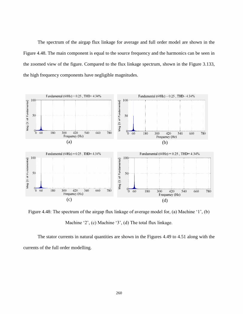
The spectrum of the airgap flux linkage for average and full order model are shown in the
Figure 4.48. The main component is equal to the source frequency and the harmonics can be seen in
the zoomed view of the figure. Compared to the flux linkage spectrum, shown in the Figure 3.133,
the high frequency components have negligible magnitudes.
(a)
(b)
(c)
(d)
Figure 4.48: The spectrum of the airgap flux linkage of average model for, (a) Machine ‘1’, (b)
Machine ‘2’, (c) Machine ‘3’, (d) The total flux linkage.
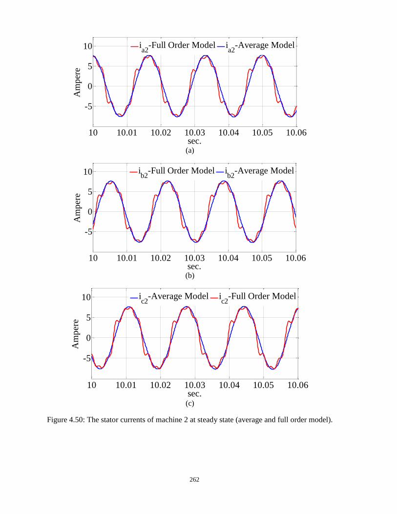
The stator currents in natural quantities are shown in the Figures 4.49 to 4.51 along with the
currents of the full order modelling.

261
(a)
(b)
(c)
Figure 4.49: The stator currents of machine 1 at steady state (average and full order model).
10 10.01 10.02 10.03 10.04 10.05 10.06
-5
0
5
10
sec.
Am
per
e
ia1
-Full Order Model ia1
-Average Model
10 10.01 10.02 10.03 10.04 10.05 10.06
-5
0
5
10
sec.
Am
per
e
ib1
-Average Model ib1
-Full Order Model
10 10.01 10.02 10.03 10.04 10.05 10.06
-5
0
5
10
sec.
Am
per
e
i c 1
-Average Model i c 1
-Full Order Model
262
(a)
(b)
(c)
Figure 4.50: The stator currents of machine 2 at steady state (average and full order model).
10 10.01 10.02 10.03 10.04 10.05 10.06
-5
0
5
10
sec.
Am
per
e
ia2
-Full Order Model ia2
-Average Model
10 10.01 10.02 10.03 10.04 10.05 10.06
-5
0
5
10
sec.
Am
per
e
ib2
-Full Order Model ib2
-Average Model
10 10.01 10.02 10.03 10.04 10.05 10.06
-5
0
5
10
sec.
Am
per
e
ic2
-Average Model ic2
-Full Order Model

263
(a)
(b)
(c)
Figure 4.51: The stator currents of machine 3 at steady state (average and full order model).
The stator current in the stationary reference frame are also shown in Figure 4.52. This
Figure shows the First, third, Fifth and seventh sequence currents of the stationary reference frame.
10 10.01 10.02 10.03 10.04 10.05 10.06
-5
0
5
10
sec.
Am
per
e
ia3
-Full Order Model ia3
-Average Model
10 10.01 10.02 10.03 10.04 10.05 10.06
-5
0
5
10
sec.
Am
per
e
ib3
-Full Order Model ib3
-Average Model
10 10.01 10.02 10.03 10.04 10.05 10.06
-5
0
5
10
sec.
Am
per
e
ic3
-Average Model ic3
-Full Order Model

264
(a)
(b)
(c)
(d)
Figure 4.52: The stator currents in stationary reference frame in, (a) First sequence, (b) Third
sequence, (c) Fifth sequence, (d) Seventh sequence.
4.6 Decoupling the Average Model of the Symmetrical and Asymmetrical Triple-Star IPM
Machines
4.6.1 Background
Generally, a linear system can be defined as:
)()()(
)()()(
tDUtCxty
tBUtAxtx
(4.54)
In this equation ‘A’ represents the system matrix, ‘B’ is the input matrix, ‘U’ is the input of
the system, ‘C’ is the output matrix and ‘X’ represents the state vector of the system [160]. The
couplings between the state variables are due to the non-diagonal terms of the matrix ‘A’. To decouple
the state variables from each other, the system needs to be transformed to a decoupled form. The
10 10.01 10.02 10.03 10.04 10.05 10.06
-5
0
5
10
sec.
Am
per
e
iq1
id1
10 10.01 10.02 10.03 10.04 10.05 10.06
-0.5
0
0.5
sec.
Am
per
e
iq3
id3
10 10.01 10.02 10.03 10.04 10.05 10.06
-0.2
0
0.2
0.4
sec.
Am
per
e
iq5
id5
10 10.01 10.02 10.03 10.04 10.05 10.06-0.1
-0.05
0
0.05
0.1
0.15
sec.
Am
per
e
iq7
id7

265
transformation to the new form is basically multiplying the system by a decoupling matrix. The
decoupling matrix can be generated from the matrix ‘A’. An n×n matrix like ‘A’ with distinct eigen
values is called diagonalizable if there exists an invertible matrix like P such that the APP 1 is
diagonal [160].
By considering the eigen values of the matrix A as nii ,....3,2,1, , then for each
eigen value there will be an associated eigen vector given as niqi ,....3,2,1, such that:
iii qAq (4.55)
The set of the eigen vectors are linearly independent, therefore they can be used as a base to
represent ‘A’ in a new form called ‘ A ’. When ‘ A ’ is the representation of the matrix ‘A’ with the
respect of the niqi ,....3,2,1, basis, then the first column of ‘ A ’ is the representation of
111 qAq with respect to the 1q .
0
.
0...
1
21111
nqqqqAq
(4.56)
It means the first column of the ‘ A ’ can be defined as:
0
.
0
1
1
V
(4.57)
266
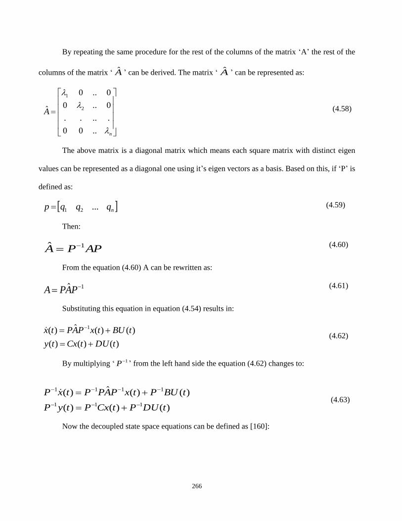
By repeating the same procedure for the rest of the columns of the matrix ‘A’ the rest of the
columns of the matrix ‘ A ’ can be derived. The matrix ‘ A ’ can be represented as:
n
A
..00
.....
0..0
0..0
ˆ 2
1
(4.58)
The above matrix is a diagonal matrix which means each square matrix with distinct eigen
values can be represented as a diagonal one using it’s eigen vectors as a basis. Based on this, if ‘P’ is
defined as:
nqqqp ...21 (4.59)
Then:
APPA 1ˆ (4.60)
From the equation (4.60) A can be rewritten as:
1ˆ PAPA (4.61)
Substituting this equation in equation (4.54) results in:
)()()(
)()(ˆ)( 1
tDUtCxty
tBUtxPAPtx
(4.62)
By multiplying ‘ 1P ’ from the left hand side the equation (4.62) changes to:
)()()(
)()(ˆ)(
111
1111
tDUPtCxPtyP
tBUPtxPAPPtxP
(4.63)
Now the decoupled state space equations can be defined as [160]:

267
)(')(')('
)(')('ˆ)('
tUDtxCty
tUBtxAtx
(4.64)
Where:
DPDCPCBPBtxPtx 1111 ',','),()(' (4.65)
4.6.2 Decoupling the Machine Model
As it can be seen from the equation (4.37) there are some coupling terms between the different
machines inductances. The coupling terms are actually the non-diagonal terms of the inductance
matrix. These inductances can cause some complexity in designing the controller for the machine
[140]. To remove these coupling terms, a new reference frame is needed to be presented. The
transformation will be a combination of the rotor reference frame transformation and a second
transformation that can make the inductance matrix of equation (4.35) diagonal. The procedure of
finding the new transformation can start from diagonalzing the matrix of equation (4.35). To be able
to determine the diagonal matrix of the inductances, the matrix should have distinct eigen values
[143]. To have distinct Eigen values the zero sequence inductances should be removed, therefore the
inductance matrix can shrink to the matrix of equation (4.66).
d
q
md
mq
md
mq
md
mq
d
q
md
mq
md
mq
md
mq
d
q
dd
dd
dd
dd
dd
dd
dd
dd
dd
qd
L
L
L
L
L
L
L
L
L
L
L
L
L
L
L
L
L
L
L
L
L
L
L
L
L
L
L
L
L
L
L
L
L
L
L
L
L
0
0
0
0
0
0
0
0
0
0
0
0
0
0
0
0
0
0
0
0
0
0
0
0
0
0
0
0
0
0
0
0
0
0
0
0
33
33
23
23
31
31
32
32
22
22
12
12
31
31
21
21
11
11
(4.66)

268
Generally, a matrix like qdL is diagnosable if there exists an invertible matrix like P such
that the PLP qd
1 is invertible [147].
P
L
L
L
L
L
L
L
L
L
L
L
L
L
L
L
L
L
L
PL
dd
dd
dd
dd
dd
dd
dd
dd
dd
qdn
33
33
23
23
31
31
32
32
22
22
12
12
31
31
21
21
11
11
1
0
0
0
0
0
0
0
0
0
0
0
0
0
0
0
0
0
0
(4.67)
Where: ‘P’, is a matrix formed by the eigen vectors of the main matrix ( qdL ).
654321 VVVVVVP
(4.68)
To obtain the eigen vectors of the matrix, the eigen values are needed. The eigen values can
be calculated as:
0 ILqd
0
100000
010000
001000
000100
000010
000001
0
0
0
0
0
0
0
0
0
0
0
0
0
0
0
0
0
0
33
33
23
23
31
31
32
32
22
22
12
12
31
31
21
21
11
11
dd
dd
dd
dd
dd
dd
dd
dd
dd
L
L
L
L
L
L
L
L
L
L
L
L
L
L
L
L
L
L
(4.69)
The last equation is equal to:
0
0
0
0
0
0
0
0
0
0
0
0
0
0
0
0
0
0
0
33
33
23
23
31
31
32
32
22
22
12
12
31
31
21
21
11
11
dd
dd
dd
dd
dd
dd
dd
dd
dd
L
L
L
L
L
L
L
L
L
L
L
L
L
L
L
L
L
L
(4.70)

269
Using the MATLAB (Symbolic Toolbox), the eigen values of the matrix are.
31111 qqqq LL
31112 dddd LL
2
8
2
312
212
31
113
qqqqqq
LLLL
2
8
2
312
212
31
114
qqqqqq
LLLL
2
8
2
312
212
31115
dddddddd
LLLL
2
8
2
312
212
31116
dddddddd
LLLL
(4.71)
Using the eigen values the eigen vectors ( iV ) of the matrix can be derived as:
0 ii VIA
(4.72)
Therefore, the eigen vectors corresponding to each of the eigen values are given in equations
(4.73) to (4.77).
0
1
0
85.05.0
0
1
21
3111312
212
3111
1 qq
qqqqqqqqqqqq
L
LLLLLL
V
(4.73)
0
1
0
85.05.0
0
1
21
3111312
212
3111
2 qq
qqqqqqqqqqqq
L
LLLLLL
V
(4.74)

270
0
1
0
0
0
1
3V ,
1
0
0
0
1
0
4V
(4.75)
1
0
85.05.0
0
1
0
21
3111312
212
31115
dd
dddddddddddd
L
LLLLLLV
(4.76)
1
0
85.05.0
0
1
0
21
3111312
212
31116
dd
dddddddddddd
L
LLLLLLV
(4.77)
Substituting the self and mutual inductances from the equation 4.66 into the eigen vectors,
they change to:
0
1
0
2
0
1
0
1
0
85.05.0
0
1
22
1 mq
mqqmqmqmqq
L
LLLLLL
V
(4.78)

271
0
1
0
1
0
1
0
1
0
95.05.0
0
1
2
2 mq
mqqmqmqq
L
LLLLL
V
(4.79)
0
1
0
0
0
1
3V ,
1
0
0
0
1
0
4V
(4.80)
1
0
1
0
1
0
1
0
95.05.0
0
1
0
25
md
mddmdmdd
L
LLLLLV
(4.81)
1
0
2
0
1
0
1
0
95.05.0
0
1
0
26
d
mddmdmdd
L
LLLLLV
(4.82)
Now by arranging the vectors in the same matrix, the matrix P can be formed as:

272
(4.83)
The inverse of the matrix P also can be defined as:
(4.84)
The columns of the matrix iW can be defined as:
0
0
02
1
84
8
84
8
312
212
312
212
31
312
212
312
212
31
1
qqqq
qqqqqq
qqqq
qqqqqq
LL
LLL
LL
LLL
W ,
312
212
312
212
31
312
212
312
212
31
2
84
8
84
8
2
10
0
0
dddd
dddddd
dddd
dddddd
LL
LLL
LL
LLLW
(4.85)
0
0
0
0
8
8
312
212
21
312
212
21
3
qqqq
dd
qqqq
LL
L
LL
L
W ,
312
212
21
312
212
214
8
8
0
0
0
0
dddd
dddd
dd
LL
LLL
LW
(4.86)
1
0
2
0
1
0
1
0
1
0
1
0
1
0
0
0
1
0
0
1
0
0
0
1
0
1
0
1
0
1
0
1
0
2
0
1
P
654321
1 WWWWWWP

273
0
0
02
1
84
8
84
8
312
212
312
212
31
332
212
312
212
31
5
qqqq
qqqqqq
qqqq
qqqqqq
LL
LLL
LL
LLL
W ,
312
212
312
212
31
312
212
312
212
31
6
84
8
84
8
2
10
0
0
dddd
dddddd
dddd
dddddd
LL
LLL
LL
LLLW
(4.87)
Substituting the self and mutual inductances from equation (4.66) into the vectors results in:
0
0
02
13
16
1
0
0
02
1
94
9
94
9
2
2
2
2
1
mq
mqmq
mq
mqmq
L
LL
L
LL
W ,
6
13
12
10
0
0
94
9
94
9
2
10
0
0
2
2
2
22
md
mdmd
md
mdmd
L
LL
L
LLW
(4.88)
0
0
0
03
13
1
0
0
0
0
9
9
2
2
3
mq
mq
mq
mq
L
L
L
L
W ,
3
13
10
0
0
0
9
9
0
0
0
0
2
2
4
md
md
md
md
L
LL
LW
(4.89)

274
0
0
02
13
16
1
0
0
02
1
94
9
94
9
2
2
2
2
5
mq
mqmq
mq
mqmq
L
LL
L
LL
W ,
6
13
12
10
0
0
94
9
94
9
2
10
0
0
2
2
2
26
md
mdmd
md
mdmd
L
LL
L
LLW
(4.90)
Therefore, by arranging the vectors in the same matrix, the matrix 1P can be expressed as:
(4.91)
Now using the P and 1P the inductance matrix can be diagonalized as equation (4.92).
mqq
mqq
mqq
mdd
mdd
mdd
qdqdn
LL
LL
LL
LL
LL
LL
PLPL
00000
020000
00000
00000
000020
00000
1
(4.92)
6
10
3
10
6
10
3
10
3
10
3
10
2
1000
2
10
02
1000
2
1
03
10
3
10
3
1
06
10
3
10
6
1
1P

275
By adding the leakage inductances to the self-inductances of the equations (4.26) to (4.34)
and substitute them into the equation (4.92) the inductance matrix changes to:
ls
mqls
ls
ls
mdls
ls
qdqdn
L
LL
L
L
LL
L
PLPL
00000
030000
00000
00000
000030
00000
1
(4.93)
Where: lsL represents the leakage inductance of the stator phases. Now the whole model of the
machine can be transformed to the new reference frame to get the decoupled model for the machine.
The new transformation matrix which includes the diagonalizing matrix (after inserting the zero
sequence) can be defined as:

276
2
1
2
1
2
1000000
0002
1
2
1
2
1000
0000002
1
2
1
2
1666333666
333333333
222000
222
222000
222
333333333
666333666
3
2
2
1
2
1
2
1000000
0002
1
2
1
2
1000
0000002
1
2
1
2
1
000000
000000
000000
000000
000000
000000
3
2
100000000
010000000
001000000
0006
10
3
10
6
10
0003
10
3
10
3
10
0002
1000
2
10
00002
1000
2
1
00003
10
3
10
3
1
00006
10
3
10
6
1
333222111
333222111
333111
333222
333222111
333222111
333
333
222
222
111
111
1
rrrrrrrrr
rrrrrrrrr
rrrrrr
rrrrrr
rrrrrrrrr
rrrrrrrrr
rrr
rrr
rrr
rrr
rrr
rrr
rrn
SSSSSSSSS
SSSSSSSSS
SSSSSS
CCCCCC
CCCCCCCCC
CCCCCCCCC
SSS
CCC
SSS
CCC
SSS
CCC
TPT
(4.94)

277
And also the reverse of the transformation matrix can be defined as:
100
100
100
0102002
0102002
0102002
001
001
001
100000000
010000000
001000000
000111000
000000111
000210000
000000012
000111000
000000111
1000000
1000000
1000000
0100000
0100000
0100000
0010000
0010000
0010000
333333
333333
333333
2222
2222
2222
111111
111111
111111
33
33
33
22
22
22
11
11
11
11
rrrrrr
rrrrrr
rrrrrr
rrrr
rrrr
rrrr
rrrrrr
rrrrrr
rrrrrr
rr
rr
rr
rr
rr
rr
rr
rr
rr
rrn
SSSCCC
SSSCCC
SSSCCC
SSCC
SSCC
SSCC
SSSCCC
SSSCCC
SSSCCC
SC
SC
SC
SC
SC
SC
SC
SC
SC
PTT
(4.95)

278
Where ‘C’ represents cos, ‘S’ represents sin, 9
,
3
2 and i is defined according
to Table 4.1. Now the machine equations can be transformed to the new reference frame ( nT ) as:
abciabcisabci pirV
qdnrnqdnrnsabci pTiTrV 11
qdnrnrnqdnrnsrnabcirn pTTiTrTVT 11
(4.96)
The different terms of the equation (4.96) can be represented as:
3
2
1
3
3
2
2
1
1
3
3
3
2
2
2
1
1
1
o
o
o
nd
nq
nd
nq
nd
nq
c
b
a
c
b
a
c
b
a
rnabcirn
V
V
V
V
V
V
V
V
V
V
V
V
V
V
V
V
V
V
TVT
(4.97)
3
2
1
3
3
2
2
1
1
3
3
3
2
2
2
1
1
1
o
o
o
nd
nq
nd
nq
nd
nq
c
b
a
c
b
a
c
b
a
rnabcirnqdn
i
i
i
i
i
i
i
i
i
i
i
i
i
i
i
i
i
i
TiTi
(4.98)
The last term in the equation (4.96) which includes derivation can be expanded as:

279
qdnrnrnqdnrnrnqdnrnrn pTTpTTpTT 111
(4.99)
The first term of the equation (4.99) is:
qdnr
qdnrrqdnrnrn
VVVVVVWWWWWW
PpTTPpTT
654321654321
111
(4.100)
Substituting the P , 1P and r into the equation (4.100) and inserting zero sequences,
results in:

280
(4.101)
3
2
1
3
3
2
2
1
1
3
2
1
3
3
2
2
1
1
1
000000000
000000000
000000000
000000001
000000010
000000100
000001000
000010000
000100000
100000000
010000000
001000000
000111000
000000111
000210000
000000012
000111000
000000111
000000000
000000000
000000000
000010000
000100000
000000100
000001000
000000001
000000010
100000000
010000000
001000000
0006
10
3
10
6
10
0003
10
3
10
3
10
0002
1000
2
10
00002
1000
2
1
00003
10
3
10
3
1
00006
10
3
10
6
1
do
do
do
nd
nq
nd
nq
nd
nq
r
do
do
do
nd
nq
nd
nq
nd
nq
r
qdnrnrn pTT

281
The second part of the equation (4.100) is equal to:
3
2
1
3
3
2
2
1
1
1
100000000
010000000
001000000
000100000
000010000
000001000
000000100
000000010
000000001
do
do
do
nd
nq
nd
nq
nd
nq
qdnrnrn
p
p
p
p
p
p
p
p
p
pTT
(4.102)
The resistances of the machine in the new reference frame also can be presented as:
s
s
s
s
s
s
s
s
s
rsrsn
r
r
r
r
r
r
r
r
r
PTrTPr
00000000
00000000
00000000
00000000
00000000
00000000
00000000
00000000
00000000
11
(4. 103)
Substituting the different terms of the machine in the decoupled reference frame in to the
equation (4.96) and adding zero sequences of the machines to that, results in equation (4.104).

282
ndr 1
nqV 1
nqi 1
nqr 1
ndV 1
ndi 1
3Lmq
ndr 2
nqi 2
nqr 2
ndi 2
ndr 3
nqi 3
nqr 3
ndi 3
1oV
1oi
2oV
2oi
3oV
3oi
sr
sr
sr
sr
sr
sr
lsL
lsL
lsL
lsL
lsL
lsL
lsL lsL lsLsr sr sr
nqV 2 nqV 3
ndV 2 ndV 3
3Lmd
Figure 4.53: The equivalent circuit of the machine in the rotor reference frame.
3
2
1
3
3
2
2
1
1
3
2
1
3
3
2
2
1
1
3
2
1
3
3
2
2
1
1
3
2
1
3
3
2
2
1
1
00000000
00000000
00000000
00000000
000030000
00000000
00000000
000000030
00000000
0
0
0
0
0
0
0
0
00000000
00000000
00000000
00000000
000030000
00000000
00000000
000000030
00000000
o
o
o
nd
nq
nd
nq
nd
nq
ls
ls
ls
ls
mqls
ls
ls
mdls
ls
pm
o
o
o
nd
nq
nd
nq
nd
nq
ls
ls
ls
ls
mqls
ls
ls
mdls
ls
rn
o
o
o
nd
nq
nd
nq
nd
nq
sn
o
o
o
nd
nq
nd
nq
nd
nq
i
i
i
pi
pi
pi
pi
pi
pi
L
L
L
L
LL
L
L
LL
L
i
i
i
i
i
i
i
i
i
L
L
L
L
LL
L
L
LL
L
i
i
i
i
i
i
i
i
i
r
V
V
V
V
V
V
V
V
V
(4.104)

283
And finally the voltage equations of the machine can be represented as:
0
0
0
3
3
0
0
0
3
3
000000000
000000000
000000000
000000001
000000010
000000100
000001000
000010000
000100000
3
3
2
2
1
1
3
3
2
2
1
1
3
2
1
3
3
2
2
1
1
3
2
1
3
3
2
2
1
1
ndls
nqmqls
ndls
nqls
ndmdls
nqls
ndls
nqmqls
ndls
nqls
pmndmdls
nqls
r
o
o
o
nd
nq
nd
nq
nd
nq
sn
o
o
o
nd
nq
nd
nq
nd
nq
ipL
iLLp
ipL
ipL
iLLp
ipL
iL
iLL
iL
iL
iLL
iL
i
i
i
i
i
i
i
i
i
r
V
V
V
V
V
V
V
V
V
(4.105)
The flux linkages of the machines can be represented as:
0
0
0
0
0
0
0
0
00000000
00000000
00000000
00000000
000030000
00000000
00000000
000000030
00000000
3
2
1
3
3
2
2
1
1
3
2
1
3
3
2
2
1
1
pm
o
o
o
nd
nq
nd
nq
nd
nq
ls
ls
ls
ls
mqls
ls
ls
mdls
ls
o
o
o
nd
nq
nd
nq
nd
nq
i
i
i
i
i
i
i
i
i
L
L
L
L
LL
L
L
LL
L
(4.106)
The generated torque of the machine can be calculated using the co-energy equation. The
co-energy of the machine can be presented as function of the stator currents and the flux linkages
as [122]:
pm
t
ssss
t
sco IILIW 2
1
(4.107)
Where ssL and sI are the machine inductances and current, defined as:

284
333333232323131313
333333232323131313
333333232323131313
323232222222121212
323232222222121212
323232222222121212
313131212121111111
313131212121111111
313131212121111111
ccbcacccbcacccbcac
cbbbabcbbbabcbbbab
cabaaacabaaacabaaa
ccbcacccbcacccbcac
cbbbabcbbbabcbbbab
cabaaacabaaacabaaa
ccbcacccbcacccbcac
cbbbabcbbbabcbbbab
cabaaacabaaacabaaa
ss
LLLLLLLLL
LLLLLLLLL
LLLLLLLLL
LLLLLLLLL
LLLLLLLLL
LLLLLLLLL
LLLLLLLLL
LLLLLLLLL
LLLLLLLLL
L
(4.108)
From the torque and co-energy equation, the electromagnetic torque can be derived as
[122]:
rm
coe
WT
(4.110)
From the equation (4.110), the torque can be expressed as:
rm
pmt
ss
rm
sst
se IIL
IT
2
1
(4.111)
Since the previous equations are in term of the electrical angle, the mechanical angle needs
to be converted to the electrical angle as presented in equation (4.112).
3
3
3
2
2
2
1
1
1
c
b
a
c
b
a
c
b
a
s
i
i
i
i
i
i
i
i
i
I
(4.109)

285
rmr
P
2
(4.112)
Therefore, the torque equation changes to the equation (4.113):
r
pmt
ss
r
sst
se IP
IL
IP
T
22
1
2
(4.113)
Substituting the stator currents with their corresponding values in rotor reference frame
results in:
r
pm
rn
t
qdnqdnrn
r
ssrn
t
qdne TIP
ITL
TIP
T
)()(
22
3)()()(
22
3 1
(4.114)
This equation can be rewritten as:

286
0
0
0
0
0
0
0
0
22
3
00000000
00000000
00000000
00000000
000030000
00000000
00000000
000000030
00000000
22
3
3
2
1
3
3
2
2
1
1
3
2
1
3
3
2
2
1
1
3
2
1
3
3
2
2
1
1
pm
t
o
o
o
nd
nq
nd
nq
nd
nq
o
o
o
nd
nq
nd
nq
nd
nq
ls
ls
ls
ls
mqls
ls
ls
mdls
ls
t
o
o
o
nd
nq
nd
nq
nd
nq
e
i
i
i
i
i
i
i
i
i
P
i
i
i
i
i
i
i
i
i
L
L
L
L
LL
L
L
LL
L
i
i
i
i
i
i
i
i
i
PT
(4.115)

287
The electromagnetic torque of the machine can be represented as:
pmndndnqmqndnqmd
oolslsoolsls
oolslspmnqndnqlsmqls
ndnqlslsndnqlsmdlse
iiiLiiLP
iiLLP
iiLLP
iiLLP
iP
iiLLLP
iiLLP
iiLLLP
T
13311
3231
21133
2211
4
9
)(4
3)(
4
3
)(4
3
4
3)3(
4
3
)(4
3)3(
4
3
(4.116)
The dynamic equation governing rotor speed can also be derived using the electromagnetic
and load torque. In the equation (4.117) ‘P’ is the pole pairs of the machine, ‘𝜔𝑟’ is the rotor speed,
‘B’ is the friction coefficient and ‘𝑇𝐿’ is the mechanical load torque applied to the machine.
rLre BTpP
JT
2
(4.117)
In equation (4.104) the torque producing voltages (the voltages that have inductances
bigger than the leakage) are nqV 1 and ndV 3 . The rest of the voltages are not able to produce
electromagnetic torque. To generate a simpler model, the torque producing voltages need to be
shifted to the top rows of the model matrix. The model modification can be done by modifying the
diagonalizing matrix. The new diagonalizig matrix ( 1'P and 'P ) are presented in the equations
(4.118) and (4.119) respectively. This matrix has been generated by exchanging the first and fifth
rows of the original matrix and also multiplying the first and second row to ‘-1’.

288
(4.118)
(4.119)
Using the new diagonalzing matrix and inserting the zero sequences, the new
transformation matrix can be generated as equation (4.120).
6
10
3
10
6
10
06
10
3
10
6
12
1000
2
10
02
1000
2
1
03
10
3
10
3
13
10
3
10
3
10
1'P
1
0
2
0
1
0
0
1
0
2
0
1
1
0
0
0
1
0
0
1
0
0
0
1
0
1
0
1
0
1
1
0
1
0
1
0
'P

289
2
1
2
1
2
1000000
0002
1
2
1
2
1000
0000002
1
2
1
2
1666333666
666333666
222000
222
222000
222
333333333
333333333
3
2
2
1
2
1
2
1000000
0002
1
2
1
2
1000
0000002
1
2
1
2
1
000000
000000
000000
000000
000000
000000
100000000
010000000
001000000
0006
10
3
10
6
10
00006
10
3
10
6
1
0002
1000
2
10
00002
1000
2
1
00003
10
3
10
3
1
0003
10
3
10
3
10
3
2
333222111
333222111
333111
333111
333222111
333222111
333
333
222
222
111
111
'1''
rrrrrrrrr
rrrrrrrrr
rrrrrr
rrrrrr
rrrrrrrrr
rrrrrrrrr
rrr
rrr
rrr
rrr
rrr
rrr
rrn
SSSSSSSSS
CCCCCCCCC
SSSSSS
CCCCCC
CCCCCCCCC
SSSSSSSSS
SSS
CCC
SSS
CCC
SSS
CCC
TPT
(4.120)
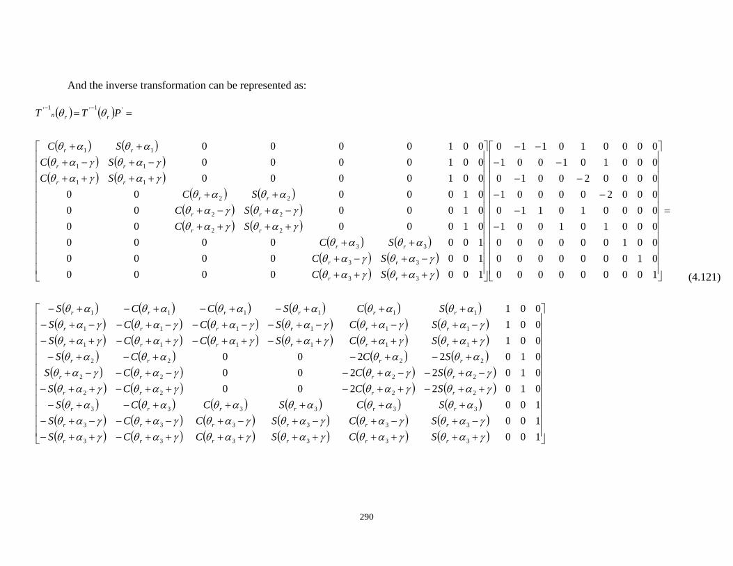
290
And the inverse transformation can be represented as:
100
100
100
0102200
0102200
0102200
001
001
001
100000000
010000000
001000000
000101001
000010110
000200001
000020010
000101001
000010110
1000000
1000000
1000000
0100000
0100000
0100000
0010000
0010000
0010000
333333
333333
333333
2222
2222
2222
111111
111111
111111
33
33
33
22
22
22
11
11
11
'1'1'
rrrrrr
rrrrrr
rrrrrr
rrrr
rrrr
rrrr
rrrrrr
rrrrrr
rrrrrr
rr
rr
rr
rr
rr
rr
rr
rr
rr
rrn
SCSCCS
SCSCCS
SCSCCS
SCCS
SCCS
SCCS
SCSCCS
SCSCCS
SCSCCS
SC
SC
SC
SC
SC
SC
SC
SC
SC
PTT
(4.121)

291
Now the machine voltage equations can be transformed to the new reference frame using
the new transformation matrix. The machine equations in natural quantities can be expressed as:
abciabcisabci pirV
(4.122)
Substituting the currents and flux linkages by their equivalent in the decoupled reference
frame results in:
qdnrnqdnrnsabci pTiTrV 1'1'
(4.123)
Multiplying the rnT 'from the left hand side, the equation changes to:
qdnrnrnqdnrnsrnabcirn pTTiTrTVT 1''1'''
(4.124)
The different components of the equation (4.124) can be represented as:
3
2
1
3
3
2
2
1
1
3
3
3
2
2
2
1
1
1
o
o
o
nd
nq
nd
nq
nd
nq
c
b
a
c
b
a
c
b
a
rnabcirn
V
V
V
V
V
V
V
V
V
V
V
V
V
V
V
V
V
V
TVT
(4.125)
3
2
1
3
3
2
2
1
1
3
3
3
2
2
2
1
1
1
o
o
o
nd
nq
nd
nq
nd
nq
c
b
a
c
b
a
c
b
a
rnabcirnqdn
i
i
i
i
i
i
i
i
i
i
i
i
i
i
i
i
i
i
TiTi
(4.126)

292
The derivative part also is equal to:
qdnrnrnqdnrnrnqdnrnrn pTTpTTpTT 1''1''1''
(4.127)
The first part of the equation (4.127) is equal to:
qdnrqdnrrqdnrnrn PPPpTTPpTT '1''11'1''
(4.128)
Substituting the'P ,
1'P and r into the equation (4.128) results in:

293
(4.129)
3
2
1
3
3
2
2
1
1
3
2
1
3
3
2
2
1
1
1
000000000
000000000
000000000
000010000
000100000
000000100
000001000
000000001
000000010
100000000
010000000
001000000
000101001
000010110
000200001
000020010
000101001
000010110
000000000
000000000
000000000
000010000
000100000
000000100
000001000
000000001
000000010
100000000
010000000
001000000
0006
10
3
10
6
10
00006
10
3
10
6
1
0002
1000
2
10
00002
1000
2
1
00003
10
3
10
3
1
0003
10
3
10
3
10
do
do
do
nd
nq
nd
nq
nd
nq
r
do
do
do
nd
nq
nd
nq
nd
nq
r
qdnrnrn pTT

294
The second part of the equation (4.127) is equal to:
3
2
1
3
3
2
2
1
1
1
100000000
010000000
001000000
000100000
000010000
000001000
000000100
000000010
000000001
do
do
do
nd
nq
nd
nq
nd
nq
qdnrnrn
p
p
p
p
p
p
p
p
p
pTT
(4.130)
The flux linkages in the decoupled reference frame can be explained as:
3,2,1,' iiLTp Pmabciabcissrndqin
(4.131)
Substituting the iabci by their equivalents in the decoupled reference frame, the flux
linkage equation can change to:
Pmabcirnqdnrnssrndqin TiTLTp '1''
(4.132)
The first term of the equation (4.132) is equal to equation (4.133).

295
3
2
1
3
3
2
2
1
1
3
2
1
3
3
2
2
1
1
'1''11'1''
00000000
00000000
00000000
00000000
00000000
00000000
00000000
000000030
000000003
100000000
010000000
001000000
000101001
000010110
000200001
000020010
000101001
000010110
00000000
00000000
00000000
000000
000000
000000
000000
000000
000000
100000000
010000000
001000000
0006
10
3
10
6
10
00006
10
3
10
6
1
0002
1000
2
10
00003
1000
2
1
00003
10
3
10
3
1
0003
10
3
10
3
10
o
o
o
nd
nq
nd
nq
nd
nq
ls
ls
ls
ls
ls
ls
ls
mqls
mdls
o
o
o
nd
nq
nd
nq
nd
nq
ls
ls
ls
dmdmd
qmqmq
mddmd
mqqmq
mdmdd
mqmqq
qdnqdqdn
L
rssrqdnrnssrn
i
i
i
i
i
i
i
i
i
L
L
L
L
L
L
L
LL
LL
i
i
i
i
i
i
i
i
i
L
L
L
LLL
LLL
LLL
LLL
LLL
LLL
iPLPiPTLTPiTLT
qd
(4.133)

296
The second part of the equation (4.132) is equal to:
0
0
0
0
0
0
0
0
0
0
0
0
0
0
100000000
010000000
001000000
0006
10
3
10
6
10
00006
10
3
10
6
1
0002
1000
2
10
00003
1000
2
1
00003
10
3
10
3
1
0003
10
3
10
3
10
1'
3
3
3
2
2
2
1
1
1
'
pm
pm
pm
pm
pmqd
pmc
pmb
pma
pmc
pmb
pma
pmc
pmb
pma
rpmqdn PT
(4.134)
The resistive term also can be transformed to decoupled reference frame as:
s
s
s
s
s
s
s
s
s
rsrsn
r
r
r
r
r
r
r
r
r
PTrTPr
00000000
00000000
00000000
00000000
00000000
00000000
00000000
00000000
00000000
'1''1'
(4.135)
Using the generated parts and by adding the zero sequence circuits to the model, the voltage
equation of the machine in the decoupled reference frame is presented in equation (4.136).

297
3
2
1
3
3
2
2
1
1
3
2
1
3
3
2
2
1
1
3
2
1
3
3
2
2
1
1
3
2
1
3
3
2
2
1
1
00000000
00000000
00000000
00000000
00000000
00000000
00000000
000000030
000000003
0
0
0
0
0
0
0
0
00000000
00000000
00000000
00000000
00000000
00000000
00000000
000000030
000000003
o
o
o
nd
nq
nd
nq
nd
nq
ls
ls
ls
ls
ls
ls
ls
mqls
mdls
pm
o
o
o
nd
nq
nd
nq
nd
nq
ls
ls
ls
ls
ls
ls
ls
mqls
mdls
rn
o
o
o
nd
nq
nd
nq
nd
nq
sn
o
o
o
nd
nq
nd
nq
nd
nq
i
i
i
pi
pi
pi
pi
pi
pi
L
L
L
L
L
L
L
LL
LL
i
i
i
i
i
i
i
i
i
L
L
L
L
L
L
L
LL
LL
i
i
i
i
i
i
i
i
i
r
V
V
V
V
V
V
V
V
V
(4.136)

298
Where the term rn is defined as:
(4.137)
The flux linkages are also defined as:
0
0
0
0
0
0
0
0
00000000
00000000
00000000
00000000
00000000
00000000
00000000
000000030
000000003
3
2
1
3
3
2
2
1
1
3
2
1
3
3
2
2
1
1
pm
o
o
o
nd
nq
nd
nq
nd
nq
ls
ls
ls
ls
ls
ls
ls
mqls
mdls
o
o
o
nd
nq
nd
nq
nd
nq
i
i
i
i
i
i
i
i
i
L
L
L
L
L
L
L
LL
LL
(4.138)
The equation for electromagnetic torque can be generated using the power balance between
the mechanical output power and the electrical input power. The equation (4.139) shows the
relationship between the input and the output power.
3
1
22
3
1
2
3
2
32
i
dindinqinqinrdinqinqindindinqins
i
dindinqinqinre
ipipiiiir
iViVP
T
(4.139)
000000000
000000000
000000000
000010000
000100000
000000100
000001000
000000001
000000010
rrn

299
ndr 1
nqV 1
nqi 1
nqr 1
ndV 1
ndi 1
3Lmq
ndr 2
nqi 2
nqr 2
ndi 2
ndr 3
nqi 3
nqr 3
ndi 3
1oV
1oi
2oV
2oi
3oV
3oi
sr
sr
sr
sr
sr
sr
lsL
lsL
lsL
lsL
lsL
lsL
lsL lsL lsLsr sr sr
nqV 2 nqV 3
ndV 2 ndV 3
3Lmd
Figure 4.54: The equivalent circuit of the machine in the decoupled reference frame.
The first term is the power loss and the derivative part is the changes of the stored energy which
are not effective on the electromagnetic torque. Therefore, using the average stored energy, the power
balance can be expressed equation (4.140).
3
1
3
1 22
3
2
3
i
dinqinqindinr
i
dindinqinqiner iiP
iViVT
(4.140)
By removing the term ‘ r ’ from the both sides of the equation (4.141) the torque equating
can be presented as:
nqpmnqndmqmd
nqndlsnqndlsnqndlsnqndls
ndnqmdlsnqpmnqndmqlse
iiiLLP
iiLiiLP
iiLiiLP
iiLLiiiLLP
T
111
33332222
11111
34
3
22
3
22
3
3322
3
(4.141)

300
4.7 Average Model of the Asymmetrical Double-Star Six-Phase IPM
In this section a double star asymmetrical six-phase IPM is modeled using the Fourier series
of the machine parameters. The modelling starts with the turn functions of the machine phases and
after generating the Fourier series of the turn function, winding function and the airgap function, the
Fourier series of the machine inductances are generated and the generated inductances are used to
derive the model of the machine in the rotor reference frame. Finally, the machine model is decoupled
to remove the coupling terms between different machines. The decoupling matrix and the new
transformation to the decoupled reference frame are generated and presented in this chapter.
4.7.1 Generating the Inductances of Six-Phase Double-Star IPM Machine
To generate the inductances of the machine the clock diagram is needed. The clock diagram of
the machine can be generated using the winding design method. The six-phase machine is composed
of two sets of three phase machines [149]. The machine totally has 24 slots and each machine covers
12 slots. Since the machine has four poles, the slot angular pitch can be calculated as:
)(3024
4180
24
180Degree
P
(4.142)
The slot between phases for each set can be calculated as:
430
120120
SBPH
(4.143)
The full coil pitch is:
122
2424
PFCP
(4.144)

301
Since the machine has concentrated windings then the belt is equal to 1. And also since the
machine is an asymmetrical one the slot between two adjacent machines is:
12
4
MSM
(4.145)
Where ‘M’ is the number of the machines sets. For the machine 1 the winding scheme is:
Table 4.3 The winding connections of set 1. C1- C1+ B1- B1+ A1- A1+
15 9 11 5 7 1
C1+ C1- B1+ B1- A1+ A1-
21 15 17 11 13 7
C1- C1+ B1- B1+ A1- A1+
3 21 23 17 19 13
C1+ C1- B1+ B1- A1+ A1-
21 15 17 11 13 7
The machine 2 has 1 slots shift from the machine 1, therefor the winding scheme for the
machine 2 is:
Table 4.4 The winding connections of set 2. C2- C2+ B2- B2+ A2- A2+
16 10 12 6 8 2
C2+ C2- B2+ B2- A2+ A2-
22 16 18 12 14 8
C2- C2+ B2- B2+ A2- A2+
16 10 24 18 20 14
C2+ C2- B2+ B2- A2+ A2-
22 16 6 24 2 20
Now using the Tables 4.3 and 4.4 the machine clock diagram can be presented as Figure 4.55.
The modeling can start from the turn functions of the machines. The turn functions for the machine 1
and 2 phases and the airgap function of the rotor are shown in the Figures 4.56, 4.57 respectively.
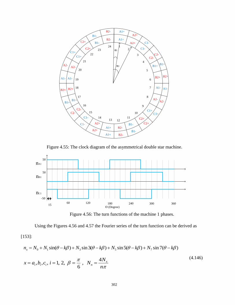
302
12
3
4
5
6
8
9
10
111213
14
15
16
17
18
19
20
21
22
2324
7
A1+
A1+
A1- A1-
A2+
A2+
A2-A2-
A1+
A1+
A2+
A2+
A1-A1-
A2-A2-
B2+ B2+
B1+B1+
B2-
B2-
B1-
B1-
B2+ B2+
B1+B1+
B1-
B1-
B2-
B2-
C1+C1+
C2+
C2+
C1-
C1-
C2-
C2-
C1+
C1+
C2+
C2+
C1-
C1-
C2-C2-
α1
α2
Figure 4.55: The clock diagram of the asymmetrical double star machine.
nA1
Ɵ (Degree)
50
50
-50
nB1
nC1
3601560 120 180 240 300
Figure 4.56: The turn functions of the machine 1 phases.
Using the Figures 4.56 and 4.57 the Fourier series of the turn function can be derived as
[153]:
)(7sin)(5sin)(3sin)sin( 75310 kNkNkNkNNnx
n
NNicbax x
niii
4,
6,2,1,,,
(4.146)

303
Where k is defined in the Table 4.5.
Ɵ (Degree)
50
50
-50
nA2
nB2
nC2
36015 60 120 180 240 300
Figure 4.57: The turn functions of the machine 2 phases.
Table 4.5 The corresponding k for the phases.
x k x k
1a 0 2a 1
1b 4 2b 5
1c 8 2c 9
The machine has the same rotor shape as the nine phase one therefore the air gap function and
the Fourier series of the inverse of the airgap function will be the same. The equation (4.3) which
shows the Fourier series of the inverse airgap function is repeated here [83].
)(14cos)(10cos)(6cos)(2cos),( 43210
1
rrrrr aaaaag (4.147)
Where: 0a , 1a , 2a , 3a and 4a are the Fourier series amplitude of the inverse air gap
function. They are given as:
aa 0 , ba 1 , 3
2
ba ,
53
ba ,
74
ba
bb gga
11
2
1,
ab ggb
11
2
1
(4.148)
Using the Fourier series of the turn functions and the airgap function and equation (4.149) [74]
the winding function of each phase can be calculated as:

304
2
0
2
0
),(
1
),(
)(
)()(
dg
dg
n
nN
r
r
w
ww
(4.149)
The different parts of the equation (4.149) can be expressed as:
2
0
0
43
2102
0
2)(14cos)(10cos
)(6cos)(2cos
),(
1ad
aa
aaad
g rr
rr
r
(4.150)
The nominator integrator also is:
2
0
0000
2
0
432107
432105
432103
432101
432100
2
0 43210
753102
0
2
)(14cos)(10cos)(6cos)(2cos)(7sin
)(14cos)(10cos)(6cos)(2cos)(5sin
)(14cos)(10cos)(6cos)(2cos)(3sin
)(14cos)(10cos)(6cos)(2cos)sin(
)(14cos)(10cos)(6cos)(2cos
)(14cos)(10cos)(6cos)(2cos
)(7sin)(5sin)(3sin)sin(
),(
)(
aNdaN
d
aaaaakN
aaaaakN
aaaaakN
aaaaakN
aaaaaN
daaaaa
kNkNkNkNNd
g
n
rrrr
rrrr
rrrr
rrrr
rrrr
rrrrr
w
(4.151)
The equations (4.149) and (4.151) result in:
22
2
),(
1
),(
)(
10
0
00
2
0
2
0 NN
a
aN
dg
dg
n
r
r
w
(4.152)
Substituting the equation (4.152) into the equation (4.146) results in:
)(7sin)(5sin)(3sin)sin(
)(7sin)(5sin)(3sin)sin()(
7531
075310
wwww
wwwww
kNkNkNkN
NkNkNkNkNNN
(4.153)
Using the generated winding function, airgap function and turn function the mutual
inductances between each couple of the windings can be calculated according to the equation (4.154).

305
2
0
75310
7531
43210
2
0
)(7sin)(5sin)(3sin)sin(
)(7sin)(5sin)(3sin)sin(
)(14cos)(10cos)(6cos)(2cos
)()(),(
1
d
kNkNkNkNN
kNkNkNkN
aaaaa
rl
dNng
rlL
iiii
jjjj
rrrr
o
ij
r
oji
(4.154)
The equation (4.153) can be simplified according the following procedure:
The winding function terms can be multiplied to the turn function according to equation
(4.1155).
2
0
75
310
7
75
310
5
75
310
3
75
310
1
43210
2
0
)(7sin)(5sin
)(3sin)sin()(7sin
)(7sin)(5sin
)(3sin)sin()(5sin
)(7sin)(5sin
)(3sin)sin()(3sin
)(7sin)(5sin
)(3sin)sin()sin(
)(14cos)(10cos)(6cos)(2cos
)()()(),(
1
d
kNkN
kNkNNkN
kNkN
kNkNNkN
kNkN
kNkNNkN
kNkN
kNkNNkN
aaaaa
rl
dNng
rlL
ii
ii
j
ii
ii
j
ii
ii
j
ii
ii
j
rrrr
o
ij
r
oji
(4.155)
The non-zero terms are:
2
0
7770
5550
3330
1110
43210
2
0
)(7sin)(7sin)(7sin
)(5sin)(5sin)(5sin
)(3sin)(3sin)(3sin
)sin()sin()sin(
)(14cos)(10cos)(6cos)(2cos
)()(),(
1
d
kkNNkNN
kkNNkNN
kkNNkNN
kkNNkNN
aaaaa
rl
dNng
rlL
ijj
ijj
ijj
ijj
rrrr
o
ij
r
oji
(4.156)

306
2
0
2
770
2
550
2
330
2
110
43210
2
0
7cos27cos2
)(7sin
5cos25cos2
)(5sin
3cos23cos2
3sin
cos2cos2
sin
)(14cos)(10cos)(6cos)(2cos
)()(),(
1
d
kkkkN
kNN
kkkkN
kNN
kkkkN
kNN
kkkkN
kNN
aaaaa
rl
dNng
rlL
ijijj
ijijj
ijijj
ijijj
rrrr
o
ij
r
oji
(4.157)
2
0
2
770
2
550
2
330
2
110
43210
2
0
7cos27cos2
)(7sin
5cos25cos2
)(5sin
3cos23cos2
3sin
cos2cos2
sin
)(14cos)(10cos)(6cos)(2cos
)()()(),(
1
d
kkkkN
kNN
kkkkN
kNN
kkkkN
kNN
kkkkN
kNN
aaaaa
rl
dNng
rlL
jiijj
jiijj
jiijj
jiijj
rrrr
o
ij
r
oji
(4.158)
Again the non-zero terms are:
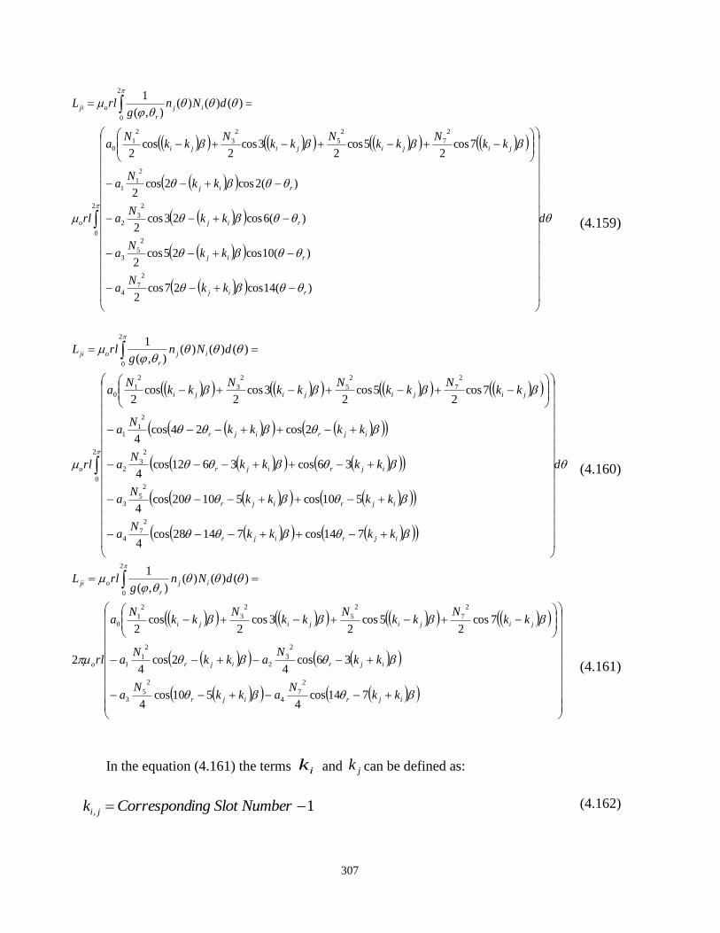
307
2
0
2
74
2
53
2
32
2
11
2
7
2
5
2
3
2
10
2
0
)(14cos27cos2
)(10cos25cos2
)(6cos23cos2
)(2cos2cos2
7cos2
5cos2
3cos2
cos2
)()()(),(
1
d
kkN
a
kkN
a
kkN
a
kkN
a
kkN
kkN
kkN
kkN
a
rl
dNng
rlL
rij
rij
rij
rij
jijijiji
o
ij
r
oji
(4.159)
2
0
2
74
2
53
2
32
2
11
2
7
2
5
2
3
2
10
2
0
714cos71428cos4
510cos51020cos4
36cos3612cos4
2cos24cos4
7cos2
5cos2
3cos2
cos2
)()()(),(
1
d
kkkkN
a
kkkkN
a
kkkkN
a
kkkkN
a
kkN
kkN
kkN
kkN
a
rl
dNng
rlL
ijrijr
ijrijr
ijrijr
ijrijr
jijijiji
o
ij
r
oji
(4.160)
ijrijr
ijrijr
jijijiji
o
ij
r
oji
kkN
akkN
a
kkN
akkN
a
kkN
kkN
kkN
kkN
a
rl
dNng
rlL
714cos4
510cos4
36cos4
2cos4
7cos2
5cos2
3cos2
cos2
2
)()()(),(
1
2
74
2
53
2
32
2
11
2
7
2
5
2
3
2
10
2
0
(4.161)
In the equation (4.161) the terms ik and jk can be defined as:
1, NumberSlotingCorrespondk ji (4.162)

308
Now using the transformation matrix of equation (4.163), the inductances can be transformed
to the rotor reference frame. The self-inductances of the machine 1 can be transformed to the rotor
reference frame as:
000
0
0
2
3
000
0
0
2
3
1
1
1
2
1
2
1
2
13
2
112110112110
1121101121102
1
112110112110
112110112110
0101101101
1011111
1011111
11
11
11
111111
111111
111111
111
111
1
11111
CaCaSaSa
SaSaCaCarlN
CLCLSLSL
SLSLCLCL
LLL
LLL
LLL
SC
SC
SC
LLL
LLL
LLL
SSS
CCC
TLTL
o
dq
dddqd
qdqqq
rr
rr
rr
ccbcac
cbbbab
cabaaa
rrr
rrr
rrqd
(4.163)
Similarly, the self-inductances of the machine 2 can be transformed to the rotor reference frame
as:
000
0
0
2
3
000
0
0
2
3
1
1
1
2
1
2
1
2
13
2
222220222220
2222202222202
1
222220222220
222220222220
0202202202
2022222
2022222
22
22
22
222222
222222
222222
222
222
1
22222
CaCaSaSa
SaSaCaCarlN
CLCLSLSL
SLSLCLCL
LLL
LLL
LLL
SC
SC
SC
LLL
LLL
LLL
SSS
CCC
TLTL
o
dq
dddqd
qdqqq
rr
rr
rr
ccbcac
cbbbab
cabaaa
rrr
rrr
rrqd
(4.164)

309
Also, the mutual inductances between the machine 1 and 2 can be transformed to the rotor
reference frame as:
000
06666
06666
2
3
000
06666
06666
2
3
1
1
1
2
1
2
1
2
13
2
212210212210
212210212210
2
1
212210212210
212210212210
0102201201
1022121
1022121
22
22
22
212121
212121
212121
111
111
1
212112
CaCaSaSa
SaSaCaCa
rlN
CLCLSLSL
SLSLCLCL
LLL
LLL
LLL
SC
SC
SC
LLL
LLL
LLL
SSS
CCC
TLTL
o
dq
dddqd
qdqqq
rr
rr
rr
ccbcac
cbbbab
cabaaa
rrr
rrr
rrqd
(4.165)
000
06666
06666
2
3
000
06666
06666
2
3
1
1
1
2
1
2
1
2
13
2
212120122120
122120122120
2
1
212120122120
122120122120
0201102102
2011212
2011212
11
11
11
121212
121212
121212
222
222
1
121221
CaCaSaSa
SaSaCaCa
rlN
CLCLSLSL
SLSLCLCL
LLL
LLL
LLL
SC
SC
SC
LLL
LLL
LLL
SSS
CCC
TLTL
o
dq
dddqd
qdqqq
rr
rr
rr
ccbcac
cbbbab
cabaaa
rrr
rrr
rrqd
(4.166)

310
To remove the mutual between q and d axis the non-diagonal terms of the inductance matrixes
in the rotor reference frame should be zero. By setting the non-diagonal terms of the matrixes in the
equations (4.165) and (4.166) to zero, the initial angels of the transformations can be calculated as:
6,0
066
066
11
212210
122120
SaSa
SaSa
(4.167)
Substituting the initial angles of the equation (4.167) in to the equations (4.163) to (4.166), the
final transformation to rotor reference frame can be expressed as:
2
1
2
1
2
1000
3
2
63
2
66000
3
2
63
2
66000
0002
1
2
1
2
1
0003
2
3
2
0003
2
3
2
3
2
rrr
rrr
rrr
rrr
r
SinSinSin
CosCosCos
SinSinSin
CosCosCos
T
(4.168)
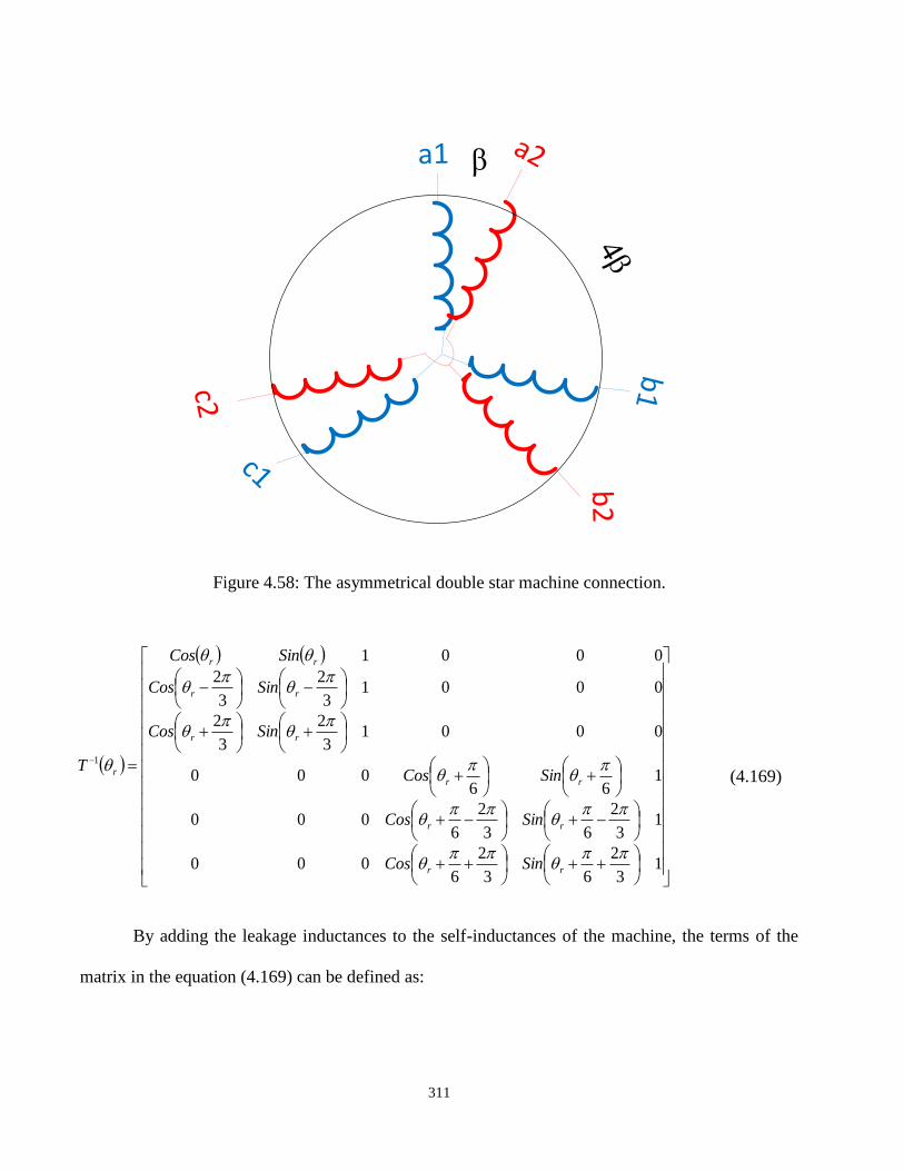
311
a1
b1
c1
a2
b2
c2
β
4β
Figure 4.58: The asymmetrical double star machine connection.
13
2
63
2
6000
13
2
63
2
6000
166
000
00013
2
3
2
00013
2
3
2
0001
1
rr
rr
rr
rr
rr
rr
r
SinCos
SinCos
SinCos
SinCos
SinCos
SinCos
T
(4.169)
By adding the leakage inductances to the self-inductances of the machine, the terms of the
matrix in the equation (4.169) can be defined as:

312
lsqlsqq
lsdlsdd
lsqlsqq
lsdlsdd
LLLLLL
LLLLLL
LLLLLL
LLLLLL
2022
2022
2011
2011
2
3
2
3
2
3
2
3
,
qqq
ddd
qqq
ddd
LLLL
LLLL
LLLL
LLLL
2012
2012
2021
2021
2
3
2
3
2
3
2
3
(4.170)
ls
dddd
qqqq
ls
dddd
qqqq
qd
L
LL
LL
L
LL
LL
L
00000
0000
0000
00000
0000
0000
2212
2212
2111
2111
(4.171)
4.7.2 Modelling of the Asymmetrical Six Phase Double Star IPM Machine
Now, the inductances and the transformation are generated so the model of the machine can
be generated. The modeling can start from the voltage equations of the stator. According to the Figure
4.58, the voltage Equations of the stator can be expressed as equation (4.172).
In this equation ‘𝐼𝑥𝑖’ is the current of phase ‘x’ and ‘𝑝𝜆𝑥’ is the derivation of the flux linkage
seen from the phase ‘x’ of the machine ‘i’ and the term ‘𝑟𝑠’ represents the stator resistance for each
phase of the stator.
cicisci
bibisbi
aiaisai
pirV
ipirV
pirV
2,1,
(4.172)
Therefore, for machine 1 the voltage equations are presented as equation (4.173).
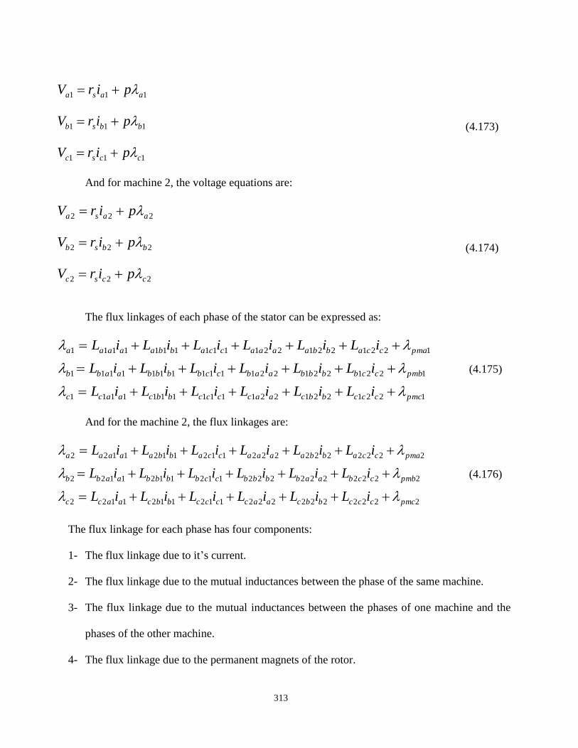
313
111
111
111
ccsc
bbsb
aasa
pirV
pirV
pirV
(4.173)
And for machine 2, the voltage equations are:
222
222
222
ccsc
bbsb
aasa
pirV
pirV
pirV
(4.174)
The flux linkages of each phase of the stator can be expressed as:
12212212211111111111
12212212211111111111
12212212211111111111
pmccccbbcaaccccbbcaacc
pmbccbbbbaabccbbbbaabb
pmaccabbaaaaccabbaaaaa
iLiLiLiLiLiL
iLiLiLiLiLiL
iLiLiLiLiLiL
(4.175)
And for the machine 2, the flux linkages are:
22222222221121121122
22222222221121121122
22222222221121121122
pmccccbbcaaccccbbcaacc
pmbccbaabbbbccbbbbaabb
pmaccabbaaaaccabbaaaaa
iLiLiLiLiLiL
iLiLiLiLiLiL
iLiLiLiLiLiL
(4.176)
The flux linkage for each phase has four components:
1- The flux linkage due to it’s current.
2- The flux linkage due to the mutual inductances between the phase of the same machine.
3- The flux linkage due to the mutual inductances between the phases of one machine and the
phases of the other machine.
4- The flux linkage due to the permanent magnets of the rotor.

314
In this equations the terms ‘𝐿𝑥𝑖𝑥𝑖’ represents the self-inductance of the phase ‘x’ of the machine
‘i’ and ‘𝐿𝑥𝑖𝑦𝑗’ represents the mutual inductance between phase ‘x’ and of the machine ‘i’ and phase
‘y’ of the machine ‘j’. Also the term ‘𝜆𝑝𝑚𝑥𝑖’ represents the flux linkage due to the permanent magnets
of the rotor seen from the phase ‘x’ of the machine ‘i’. The flux linkages can be represented in the
matrix form as:
2
2
2
1
1
1
2
2
2
1
1
1
222222121212
222222121212
222222121212
212121111111
212121111111
212121111111
pmc
pmb
pma
pmc
pmb
pma
c
b
a
c
b
a
ccbcacccbcac
cbbbabcbbbab
cabaaacabaaa
ccbcacccbcac
cbbbabcbbbab
cabaaacabaaa
pmabciabcissabci
i
i
i
i
i
i
LLLLLL
LLLLLL
LLLLLL
LLLLLL
LLLLLL
LLLLLL
iL
(4.177)
The equation (4.177) can be transformed to the rotor reference frame according to the below
procedure:
2,1, ipirV abciabcisabci (4.178)
The abc currents and the flux linkage of the equation (4.178) can be replaced by their
corresponding values in the rotor reference frame to get the equation (4.179).
2,1,11 ipTiTrV qdoirqdoirsabci (4.179)
By multiplying the rT from the left side of the equation the equation (4.179) changes to:
2,1,11 ipTTiTrTVT qdoirrqdoirsrabcir (4.180)
The different parts of the equation (4.180) can be represented as:

315
2
2
2
1
1
1
2
2
2
1
1
1
2
1
2
1
2
1000
3
2
63
2
66000
3
2
63
2
66000
0002
1
2
1
2
1
0003
2
3
2
0003
2
3
2
3
2
o
d
q
o
d
q
c
b
a
c
b
a
rrr
rrr
rrr
rrr
abcir
V
V
V
V
V
V
V
V
V
V
V
V
SinSinSin
CosCosCos
SinSinSin
CosCosCos
VT
(4.181)
The resistive part is:
s
srsr rTrT
100000
010000
001000
000100
000010
000001
1
(4.182)
The term with derivation can be expanded as:
qdoirrqdoirrqdoirr pTTpTTpTT 111
(4.183)
The first part of the equation (4.184) is expanded as:

316
qdoi
rr
rr
rr
rr
rr
rr
rrr
rrr
rrr
rrr
qdoirr
SinCos
SinCos
SinCos
SinCos
SinCos
SinCos
p
SinSinSin
CosCosCos
SinSinSin
CosCosCos
pTT
13
2
63
2
6000
13
2
63
2
6000
166
000
00013
2
3
2
00013
2
3
2
0001
2
1
2
1
2
1000
3
2
63
2
66000
3
2
63
2
66000
0002
1
2
1
2
1
0003
2
3
2
0003
2
3
2
3
2
1
(4.184)

317
By applying the derivative part and simplifying equation (4.184), it results in equation (4.185).
qdoirqdoi
rr
rr
rr
rr
rr
rr
r
rrr
rrr
rrr
rrr
qdoirr
CosSin
CosSin
CosSin
CosSin
CosSin
CosSin
SinSinSin
CosCosCos
SinSinSin
CosCosCos
pTT
000000
001000
010000
000000
000001
000010
03
2
63
2
6000
03
2
63
2
6000
066
000
00003
2
3
2
00003
2
3
2
0000
2
1
2
1
2
1000
3
2
63
2
66000
3
2
63
2
66000
0002
1
2
1
2
1
0003
2
3
2
0003
2
3
2
3
2
1
(4.185)
And the second part of the equation (4.183) is expanded as equation (4.186).

318
qdoiqdoi
rr
rr
rr
rr
rr
rr
rrr
rrr
rrr
rrr
qdoirr
pp
SinCos
SinCos
SinCos
SinCos
SinCos
SinCos
SinSinSin
CosCosCos
SinSinSin
CosCosCos
pTT
100000
010000
001000
000100
000010
000001
13
2
63
2
6000
13
2
63
2
6000
166
000
00013
2
3
2
00013
2
3
2
0001
2
1
2
1
2
1000
3
2
63
2
66000
3
2
63
2
66000
0002
1
2
1
2
1
0003
2
3
2
0003
2
3
2
3
2
1
(4.186)

319
The flux linkage of the machine can also be presented as below.
abcipmrabcissrqdoi TiLT _
(4.187)
Substituting the currents by their corresponding currents in the rotor reference frame results
in:
abcipmrqdorssrqdoi TiTLT _
1
(4.188)
The flux linkage due to the permanent magnet of the machine in the stator phases can be
transformed to the rotor reference frame according to equation (4.189). In this equation since the d
axis of the machine 1 and 2 are aligned with the flux linkage of the permanent magnet seen from the
machine 1 and 2, the flux linkage of the permanent magnet in the q axis will be zero.
0
0
0
0
2
1
2
1
2
1000
3
2
63
2
66000
3
2
63
2
66000
0002
1
2
1
2
1
0003
2
3
2
0003
2
3
2
3
2
2
2
1
1
2
2
2
1
1
1
_
pm
pm
pmo
pmd
pmq
pmo
pmd
pmq
pmc
pmb
pma
pmc
pmb
pma
rrr
rrr
rrr
rrr
abcipmr
SinSinSin
CosCosCos
SinSinSin
CosCosCos
T
(4.189)
The equation (4.188) also has a term which includes ‘𝐿𝑠𝑠’ and represents the inductances of
the stator of the machine. The inductances can be transformed to the rotor reference frame as equation
(4.190).
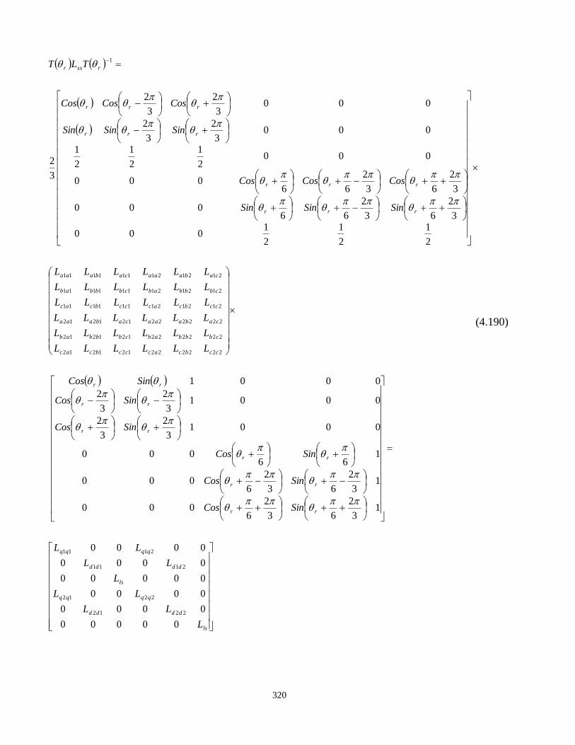
320
ls
dddd
qqqq
ls
dddd
qqqq
rr
rr
rr
rr
rr
rr
ccbcacccbcac
cbbbabcbbbab
cabaaacabaaa
ccbcacccbcac
cbbbabcbbbab
cabaaacabaaa
rrr
rrr
rrr
rrr
rssr
L
LL
LL
L
LL
LL
SinCos
SinCos
SinCos
SinCos
SinCos
SinCos
LLLLLL
LLLLLL
LLLLLL
LLLLLL
LLLLLL
LLLLLL
SinSinSin
CosCosCos
SinSinSin
CosCosCos
TLT
00000
0000
0000
00000
0000
0000
13
2
63
2
6000
13
2
63
2
6000
166
000
00013
2
3
2
00013
2
3
2
0001
2
1
2
1
2
1000
3
2
63
2
66000
3
2
63
2
66000
0002
1
2
1
2
1
0003
2
3
2
0003
2
3
2
3
2
2212
2212
2111
2111
222222121212
222222121212
222222121212
212121111111
212121111111
212121111111
1
(4.190)

321
Then, using the permanent magnet flux linkages and the inductances of the machine in the
rotor reference frame, the flux linkages of the machines in equation (4.188), can be represented in
rotor reference frame as below:
22
21122222
1122222
11
12211111
2211111
olso
pmdddddddd
qqqqqqq
olso
pmdddddddd
qqqqqqq
iL
iLiL
iLiL
iL
iLiL
iLiL
(4.191)
Also the voltages and the currents of the machines can be transformed to the rotor reference
frame as:
2
2
2
1
1
1
12
2
2
2
1
1
1
c
b
a
c
b
a
rsr
o
d
q
o
d
q
i
i
i
i
i
i
TiT
i
i
i
i
i
i
(4.192)
Using the different components of the machines the voltage equations of the machine can be
presented as equation (4.193).

322
0
0
0
0
00000
0000
0000
00000
0000
0000
0
0
0
0
00000
0000
0000
00000
0000
0000
2
2
2
1
1
1
2212
2212
2111
2111
2
2
2
1
1
1
2212
2212
2111
2111
2
2
2
1
1
1
2
2
2
1
1
1
pm
pm
o
d
q
o
d
q
ls
dddd
qqqq
ls
dddd
qqqq
pm
pm
o
d
q
o
d
q
ls
dddd
qqqq
ls
dddd
qqqq
r
o
d
q
o
d
q
s
o
d
q
o
d
q
i
i
i
i
i
i
L
LL
LL
L
LL
LL
p
i
i
i
i
i
i
L
LL
LL
L
LL
LL
i
i
i
i
i
i
r
V
V
V
V
V
V
(4.193)
The equivalent circuit if the machine for different axis are shown in the Figures 4.59 to 4.61.
rs
Lq1q1
Lls
1dr
1qV
1qi rsLls2qr
2qV
2qi
Lq2q221qqL
Figure 4.59: The equivalent circuit of the q axis.
1qr
1dV
Ld2d2
rsLls
2qr
2dV
2di
Ld1d1
rs Lls 1di
21ddL
Figure 4.60: The equivalent circuit of the d axis.

323
1oV
rs Lls1oi
2oV
rs Lls2oi
Figure 4.61: The equivalent circuit of the zero sequence.
The equation for electromagnetic torque can be generated using the power balance between
the mechanical output power and the electrical input power. The equation (4.194) shows the
relationship between the input and the output power [152].
2
1
22
2
1
2
3
2
32
i
didiqiqirdiqiqididiqis
i
didiqiqire
ipipiiiir
iViVP
T
(4.194)
The first term is the power loss and the derivative part is the changings of the stored energy
which are not effective on the electromagnetic torque, therefore using the average stored energy, the
torque can be expressed as equation (4.195).

324
31122222112222
12211111221111
31122222112222
12211111221111
2
1
2
1
22
3
22
3
22
3
22
3
2
3
dqqqqqqqpmdddddd
dqqqqqqqpmdddddd
dqqqqqqqpmdddddd
dqqqqqqqpmdddddd
i
diqiqidi
i
didiqiqie
iiLiLiiLiL
iiLiLiiLiLP
iiLiLiiLiLP
iiLiLiiLiLP
iiP
iViVT
(4.195)
4.8 Decoupling the Model
From equation (4.193) it can be seen that there are coupling terms between different machines
q and d axis (The off-diagonal terms are not zero). To remove the couplings, a new transformation is
needed. The new transformation is a combination of two different transformations, the rotor reference
frame and decoupled reference frame transformation. The decoupled transformation can be derived
by diagonalzing the matrix of the machine inductances in the rotor reference frame. The diagonalizing
procedure can be done by finding the matrix P such that the equation (4.196) is diagonal. It should be
noted that the zero sequence inductances need to be neglected to let the inductance matrix have distinct
eigen values to be diagonalizable [144].
P
LL
LL
LL
LL
PPTLTPL
dddd
qqqq
dddd
qqqq
L
rssrqdn
qd
2212
2212
2111
2111
111
00
00
00
00
(4.196)
The matrix P is built from the eigen vectors of the inductance matrix.
4321 VVVVP (4.197)

325
To obtain the eigen vectors, the eigen values are needed, the eigen values can be calculated
according to the equation (4.198).
0
00
00
00
00
0
1000
0100
0010
0001
00
00
00
00
0
1212
1111
2111
2111
2212
2212
2111
2111
dddd
qqqq
dddd
qqqq
dddd
qqqq
dddd
qqqq
qd
LL
LL
LL
LL
LL
LL
LL
LL
IL
(4.198)
The eigen values of the last matrix in the equation (4.198) are equal to:
lsqqqqqq LLLLLLLLLL 1120202021111 232
3
2
3
lsdddddd LLLLLLLLLL 1120202021112 232
3
2
3
lsqqqq LLLLLLL 2020211132
3
2
3
lsdddd LLLLLLL 2020211142
3
2
3
(4.199)
Using the eigen values, the eigen vectors of the matrix can be obtained as:
0 ii VIA (4.200)
Therefore, the eigenvectors corresponding to each of the eigen values are presented in equation
(4.201).

326
1
0
1
0
1V
0
1
0
1
2V
1
0
1
0
3V
0
1
0
1
4V
(4.201)
Using the eigen vectors, the matrix P can be formed as:
0101
1010
0101
1010
P
(4.202)
From the P the matrix, 1P also can be obtained as:
0101
1010
1010
0101
2
11P
(4.203)
Now using the generated P, the new transformation matrix can be developed as equation
(4.204).

327
3
2
63
2
663
2
3
2
3
2
63
2
663
2
3
2
3
2
63
2
663
2
3
2
3
2
63
2
663
2
3
2
3
1
3
2
63
2
66000
3
2
63
2
66000
0003
2
3
2
0003
2
3
2
0101
1010
1010
0101
3
1
1
rrrrrr
rrrrrr
rrrrrr
rrrrrr
rrr
rrr
rrr
rrr
rrn
CosCosCosCosCosCos
SinSinSinSinSinSin
SinSinSinSinSinSin
CosCosCosCosCosCos
SinSinSin
CosCosCos
SinSinSin
CosCosCos
TPT
(4.204)

328
3
2
63
2
63
2
63
2
6
3
2
63
2
63
2
63
2
6
6666
3
2
3
2
3
2
3
2
3
2
3
2
3
2
3
2
0101
1010
0101
1010
3
2
63
2
600
3
2
63
2
600
6600
003
2
3
2
003
2
3
2
00
11
rrrr
rrrr
rrrr
rrrr
rrrr
rrrr
rr
rr
rr
rr
rr
rr
rrn
CosSinCosSin
CosSinCosSin
CosSinCosSin
CosSinCosSin
CosSinCosSin
CosSinCosSin
SinCos
SinCos
SinCos
SinCos
SinCos
SinCos
PTT
(4.205)

329
Now using the new transformation, the machine voltage equation can be transformed to
the decoupled reference frame. The machine equations are presented in equation (4.172). By
substituting currents and flux linkages by their corresponding values in the decoupled reference
frame (equation (4.206)), the voltage equation changes to the equation (4.207).
qdnrnabciqdnrnabci TiTi 11 ,
(4.206)
2,1,11
ipTiTrV qdnrnqdnrnsabci (4.207)
By multiplying rnT from the left side of the equation (4.207), this equation changes to:
qdnrdnrnqdnrnsrnabcirn pTTiTrTVT 11
(4.208)
The different parts of the equation (4.208) can be expanded following:
The voltages in decoupled reference frame are:
nd
nq
nd
nq
c
b
a
c
b
a
rnabcirn
V
V
V
V
V
V
V
V
V
V
TVT
2
2
1
1
2
2
2
1
1
1
(4.209)
The currents in decoupled reference frame are:
nd
nq
nd
nq
c
b
a
c
b
a
rnabcirn
i
i
i
i
i
i
i
i
i
i
TiT
2
2
1
1
2
2
2
1
1
1
(4.210)
The resistive part of the equation (4.208) presented in equation (4.211).

330
s
s
s
s
rsrrnsrnsn
r
r
r
r
PTrTPTrTr
000
000
000
000
111
(4.211)
The last term in the equation (4.208), which includes derivation, can be expanded as:
qdnrnrnqdnrnrnqdnrnrn pTTpTTpTT 111
(4.212)
The first term of the equation (4.212) is:
qdnr
qdnr
qdnrrqdnrnrn
r
pTTPpTT
0100
1000
0001
0010
0101
1010
0101
1010
0100
1000
0001
0010
0101
1010
1010
0101
2
111
(4.213)
Also, the second term of the equation (4.212) is:
qdnqdnrnrn ppTT
1000
0100
0010
0001
1
(4.214)
The flux linkage in the decoupled reference frame can be obtain according to equation
(4.215).

331
Pmabciabcissrnabcirnqdn iLTT (4.215)
By substituting the currents from the equation (4.214) in to the equation (4.215) flux
linkages can be expressed as:
Pmabcirnqdnrnssrnabcirnqdn TiTLTT 1 (4.216)
The first term of the equation (4.216) is equal to:
qdnrn
ccbcacccbcac
cbbbabcbbbab
cabaaacabaaa
ccbcacccbcac
cbbbabcbbbab
cabaaacabaaa
rn
qdnrnssrn
iT
LLLLLL
LLLLLL
LLLLLL
LLLLLL
LLLLLL
LLLLLL
T
iTLT
1
222222121212
222222121212
222222121212
212121111111
212121111111
212121111111
1
(4.217)
The inductance matrix in the decoupled reference frame is equal to:
ls
ls
lsdd
lsqq
rn
ccbcacccbcac
cbbbabcbbbab
cabaaacabaaa
ccbcacccbcac
cbbbabcbbbab
cabaaacabaaa
rn
L
L
LL
LL
T
LLLLLL
LLLLLL
LLLLLL
LLLLLL
LLLLLL
LLLLLL
T
000
000
0020
0002
11
11
1
222222121212
222222121212
222222121212
212121111111
212121111111
212121111111
(4.218)

332
The second part of equation (4.216) (permanent magnet flux linkages seen from the stator phases, transformed to the decoupled
reference frame) can be expanded as:
0
0
0
0
0
0101
1010
1010
0101
2
1
0101
1010
1010
0101
2
1
3
2
63
2
66000
3
2
63
2
66000
0003
2
3
2
0003
2
3
2
0101
1010
1010
0101
3
1
2
2
1
1
2
2
2
1
1
1
2
2
2
1
1
1
1
2
2
2
1
1
1
pm
pm
pm
pmd
pmq
pmd
pmq
pmc
pmb
pma
pmc
pmb
pma
rrr
rrr
rrr
rrr
pmc
pmb
pma
pmc
pmb
pma
r
pmc
pmb
pma
pmc
pmb
pma
rnpmn
SinSinSin
CosCosCos
SinSinSin
CosCosCos
TPT
(4.219)

333
Therefore, the total flux linkage of the machines in the decoupled reference frame can be
represented as:
0
0
0
000
000
0020
0002
2
2
1
1
11
11
2
2
1
1
pm
nd
nq
nd
nq
ls
ls
lsdd
lsqq
nd
nq
nd
nq
i
i
i
i
L
L
LL
LL
(4.220)
Substituting the generated parts into the machine voltage equation and inserting the zero
sequence circuits to that results in:
2
1
2
2
1
1
11
11
2
1
2
2
1
1
11
11
2
1
2
2
1
1
2
1
2
2
1
1
00000
00000
00000
00000
000020
000002
0
0
0
0
0
00000
00000
00000
00000
000020
000002
000000
000000
000100
001000
000001
000010
o
o
nd
nq
nd
nq
ls
ls
ls
ls
lsdd
lsqq
pm
o
o
nd
nq
nd
nq
ls
ls
ls
ls
lsdd
lsqq
r
o
o
nd
nq
nd
nq
sn
o
o
nd
nq
nd
nq
pi
pi
pi
pi
pi
pi
L
L
L
L
LL
LL
i
i
i
i
i
i
L
L
L
L
LL
LL
i
i
i
i
i
i
r
V
V
V
V
V
V
(4.221)

334
The equivalent circuit of the machine in the decoupled reference frame is shown in Figure
4.62.
ndr 1
nqV 1
nqi 1
nqr 1
ndV 1
ndi 1
2Ld1d1
nqi 2
ndi 2
1oV
1oi
2oV
2oi
sr
sr
sr
sr
lsL
lsL
lsL
lsL
lsL lsLsr sr
nqV 2
ndV 2
2Lq1q1
ndr 2
nqr 2
Figure 4.62: The equivalent circuit of the six phase machine in decoupled reference frame.
The equation for electromagnetic torque can be generated using the power balance between
the mechanical output power and the electrical input power. The bellow equation shows the
relationship between the input and the output power.
2
1
22
2
1
2
i
dindinqinqinrdinqinqindindinqins
i
dindinqinqinre
ipipiiiir
iViVP
T
(4.222)

335
The first term is the power loss and the derivative part is the changings of the stored energy
which are not effective on the electromagnetic torque generation, therefore, using the average
stored energy, the torque can be expressed as:
nqpmnqndqqddnqndlsnqndls
nqndqqlsnqpmndnqddls
i
dinqinqindinre
iiiLLPiiLiiLP
iiLLiiiLLP
iiP
T
11111112222
111111111
2
1
2
222
2
(4.223)
New transformation matrix for the new reference frame is presented as equation (4.224).

336
2
1
2
1
2
1000
0002
1
2
1
2
13
2
63
2
663
2
3
2
3
2
63
2
663
2
3
2
3
2
63
2
663
2
3
2
3
2
63
2
663
2
3
2
3
1
rrrrrr
rrrrrr
rrrrrr
rrrrrr
rn
CosCosCosCosCosCos
SinSinSinSinSinSin
SinSinSinSinSinSin
CosCosCosCosCosCos
T
(4.224)
The inverse of the transformation matrix is also presented as:
103
2
63
2
63
2
63
2
6
103
2
63
2
63
2
63
2
6
106666
013
2
3
2
3
2
3
2
013
2
3
2
3
2
3
2
01
1
rrrr
rrrr
rrrr
rrrr
rrrr
rrrr
rn
CosSinCosSin
CosSinCosSin
CosSinCosSin
CosSinCosSin
CosSinCosSin
CosSinCosSin
T
(4.225)

337
4.9 Conclusion
In this chapter first an average model for a triple-star nine phase IPM is derived for the
symmetrical and asymmetrical connections. In this model the Fourier series of the machines
parameters are used to generate the Fourier series of the machines inductances. After calculating
the inductances of the machine, the model is simulated using MATLAB Simulink and the
simulation results are presented. Finally, the model is decoupled to remove the coupling terms
between the q and d axis of the different machines. The decoupled model is also derived and
essential transformations are presented for the both symmetrical and asymmetrical machines.
Finally, an asymmetrical six phase machine is modeled using the Fourier series of the machine
parameters. The average model of the machine is presented and the model is decoupled to remove
the coupling terms between different sets of three phase machines. The essential transformation
matrixes for the new transformation are also presented in this chapter. The major contribution of
this chapter is the generation of decoupled models that can be used for designing controllers for
the multiple star machines without facing the complexities that are raised by the coupling between
different machine sets.