50

CHAPTER 4

MATHEMATICAL MODELLING

4.1 INTRODUCTION

A mathematical model usually describes a system by a set of

equations that establish relationships between the variables of the system. The

values of the variables can be practically anything. However the variables

which represent some properties of the system, has a definite range. The

actual model is the set of functions that describe the relations between the

different variables. A general approach to the mathematical modelling process

is as follows.

1. Identifying the problem and defining the terms in the problem

with diagrams.

2. Beginning with a simple model stating the assumptions.

3. Identifying the important variables and constants and

determining how they are related to each other.

4. Developing the equations that express the relationships

between the variables and constants relaxing the assumptions.

Once the model has been developed and applied to the problem, the

resulting model solution must be analysed and checked for accuracy. It may

require modifying the model for obtaining reasonable output. This refining

process should continue until obtaining a model that agrees as closely as

possible with the experimental observations.

51

4.2 IMPORTANT POINTS CONSIDERED IN MODELLING

The important points considered in the development of

mathematical model are

1. Model should be simple to build, simple to modify,

understand and to communicate its output.

2. Simulation should not necessarily be thought of as another

technique for finding optimal solutions to problems. However,

once a simulation model has been developed, a quantitative

analyst may vary certain key design parameters and observe

the effect on the output of the computer runs.

3. In ideal compressors, the suction and discharge take place at

constant pressure. Constant pressure suction or discharge is

possible only for the compressors with open head during

suction or discharge, or the compressor speed should be

maintained zero. But, both the conditions are impossible in

actual practice. The ideal compressor operation is not affected

by valve area or speed.

4. The polytropic index of compression and expansion is

constant and the value is less than adiabatic index for an ideal

compressor. But, in actual case, the polytropic index may have

any value depending on the direction of heat transfer. During

compression, it is assumed that the surrounding temperature is

less than the air temperature and heat transfer from the air to

the surrounding makes an index of compression less than

adiabatic index, for ideal case. In the actual case, at the earlier

stages of compression, the wall temperature will be greater

than the air temperature and the heat will be transferred from

52

the wall to the air. This will make the index of compression

more than adiabatic index. Once the air temperature reaches

the wall temperature, the index of compression will be equal

to adiabatic index, and thereafter the value will be less than

adiabatic index. The same is true for index of expansion.

5. The cylinder wall temperature will not be constant along the

length of the cylinder during compression and expansion. This

will vary the heat transfer pattern and index of compression or

expansion.

6. The volume just above the valve plate is called ‘Head

volume’. The air enters the cylinder from atmosphere to the

cylinder through the head. The air first enters the head and then

to the cylinder. During suction, there will be a sudden pressure

drop on the suction side head and this greatly affects the mass of

air drawn by the compressor. Similarly, the air from the cylinder

is discharged to the delivery head and then to the reservoir.

There will be a pressure rise in the head and the discharge will

be between the head pressure and the cylinder pressure and not

between the discharge pressure and the cylinder pressure.

7. Since the pressure during suction is not constant, the

volumetric efficiency cannot be determined from the

discharge pressure and clearance ratio as in the ideal

compressor. It should be determined from the mass of air

drawn or mass of air delivered by the compressor per cycle.

8. The indicated power should be calculated using integration

method from pressure and volume at different crankangles.

(Area enclosed by the curves in a p-V diagram is equal to the

net work transfer or net heat transfer as per first law of

thermodynamics).

53

9. Hitting of valve on valve stop by sudden opening, may make

the valve to vibrate. The valve will get stabilised only after

some degrees of crankangle rotation. This phenomenon may

reduce the mass of air discharged. This loss is dependent on

the velocity of valve with which it hits the stop.

10. The temperature of air entering the cylinder will not be at

atmospheric temperature. The air enters the cylinder from the

hot head chamber. There will be heating of the incoming air

and this will reduce the volumetric efficiency. In addition,

there will be an increase in indicated power due to increased

initial temperature of air during compression.

11. The discharge coefficient cannot be taken as constant during

discharge process or suction process. It varies with valve lift,

pressure ratio and the compressor speed.

12. Whenever the valve closes there will be a flow of some

discharged air back into the cylinder and this reduces the mass

discharged per cycle. Similarly during suction process, when the

valve closes some air would flow out of the cylinder. This will

reduce the mass drawn in per cycle. This phenomenon is called

back flow that results reducing the volumetric efficiency.

13. Blow-by losses are also considered while estimating the

volumetric efficiency.

4.3 FUNDAMENTAL EQUATIONS

The equations corresponding to the instantaneous energy balance of

the air compressor during suction, compression, re-expansion and discharge

are given below. The derivations are given in Appendix 1.

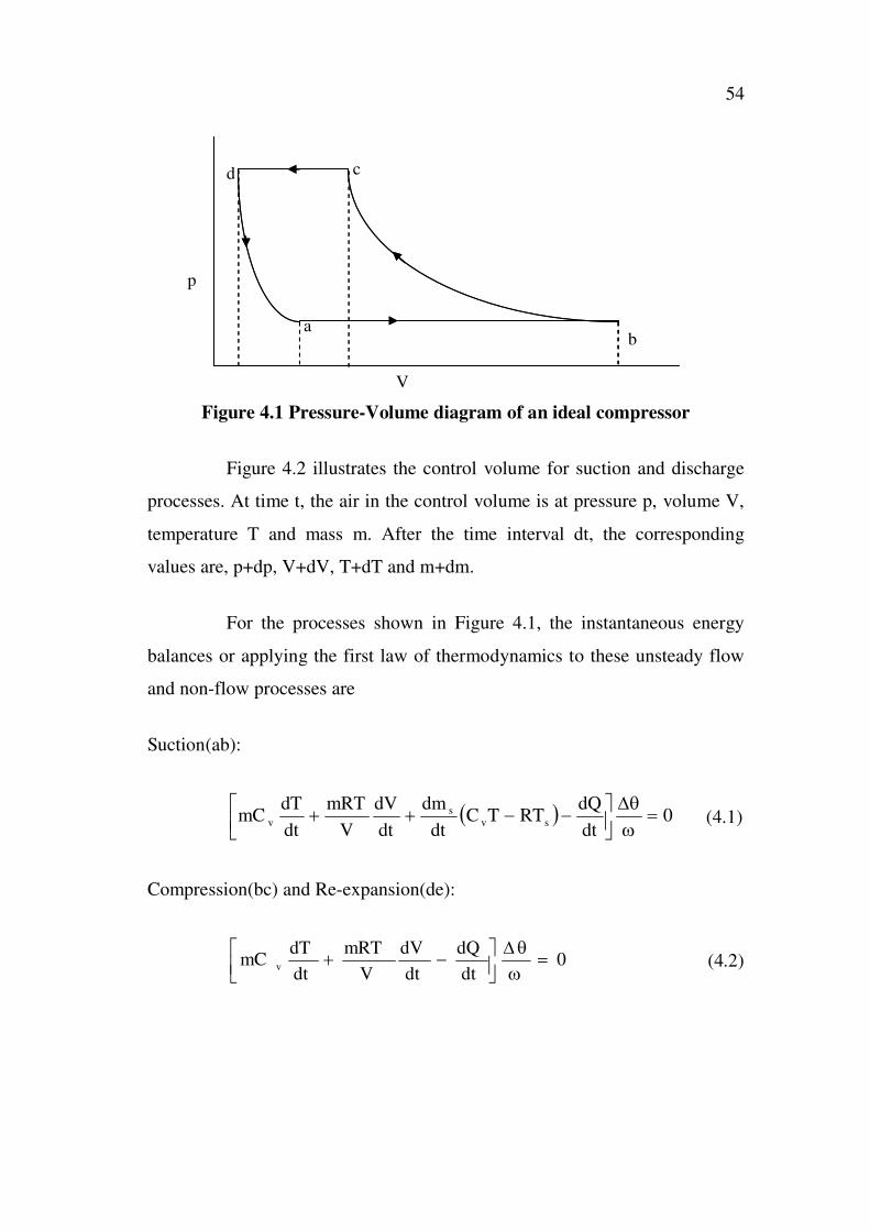
Figure 4.1 shows the p-V diagram of an ideal compressor cycle. All the

processes are assumed reversible.

54

d

p

ab

c

V

Figure 4.1 Pressure-Volume diagram of an ideal compressor

Figure 4.2 illustrates the control volume for suction and discharge

processes. At time t, the air in the control volume is at pressure p, volume V,

temperature T and mass m. After the time interval dt, the corresponding

values are, p+dp, V+dV, T+dT and m+dm.

For the processes shown in Figure 4.1, the instantaneous energy

balances or applying the first law of thermodynamics to these unsteady flow

and non-flow processes are

Suction(ab):

0dt

dQRTTC

dt

dm

dt

dV

V

mRT

dt

dTmC sv

sv (4.1)

Compression(bc) and Re-expansion(de):

0dt

dQ

dt

dV

V

mRT

dt

dTmC

v (4.2)

55

PistonPiston

t+dt t+dt

p+dp

V+dV

m+dm

T+dT

p+dp

V+dV

m+dm

T+dT

F F

dm - dm

p,V,T,m p,V,T,m

t t

Discharge(cd):

0dt

dQTCRT

dt

dm

dt

dV

V

mRT

dt

dTmC vd

dv (4.3)

4.2 a Suction process 4.2 b Discharge process

Figure 4.2 Control volume for suction and discharge processes

Governing equation for determining the instantaneous cylinder

pressure is

n

1i

ii )T(B1RT

pv (4.4)

The second term in equation (4.4) accounts for compressibility

factor and is negligible for single stage reciprocating air compressors.

Governing equation for determining the mass flow is

d

dm

d

dm

d

dm

d

dm opoi (4.5)

56

Q2

where, mop is the mass of air flowing through the gap between the piston and

the cylinder wall.

Governing equation for determining the working volume is

22

c

cc

sin)r/l(1

cossin)r/l(sin

2

LA

d

dV (4.6)

The volume of air trapped between the piston and cylinder head at

any crankangle can be determined using the properties of crank mechanism in

terms of the length of the crank lever r, the length of the connecting rod lc, the

stroke L and the cross-sectional area Ac.

The instantaneous heat transfer between the cylinder and air at any

crankangle ( ) consists of three quantities.

Q1 = Heat transfer between the air and the cylinder surface

Q2 = Heat transfer between the air and the piston surface

Q3 = Heat transfer between the air and the cylinder cover

Figure 4.3 shows the various elements of heat transfer in a

compressor.

Figure 4.3 Heat transfer in reciprocating compressor

Q1

Q3

57

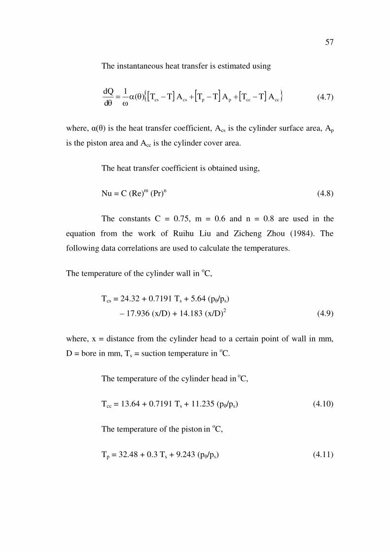
The instantaneous heat transfer is estimated using

ccccppcscs ATTATTATT)(1

d

dQ (4.7)

where, ) is the heat transfer coefficient, Acs is the cylinder surface area, Ap

is the piston area and Acc is the cylinder cover area.

The heat transfer coefficient is obtained using,

Nu = C (Re)m (Pr)

n (4.8)

The constants C = 0.75, m = 0.6 and n = 0.8 are used in the

equation from the work of Ruihu Liu and Zicheng Zhou (1984). The

following data correlations are used to calculate the temperatures.

The temperature of the cylinder wall inoC,

Tcs = 24.32 + 0.7191 Ts + 5.64 (p /ps)

– 17.936 (x/D) + 14.183 (x/D)2

(4.9)

where, x = distance from the cylinder head to a certain point of wall in mm,

D = bore in mm, Ts = suction temperature inoC.

The temperature of the cylinder head in oC,

Tcc = 13.64 + 0.7191 Ts + 11.235 (p /ps) (4.10)

The temperature of the piston inoC,

Tp = 32.48 + 0.3 Ts + 9.243 (p /ps) (4.11)

58

4.4 INDEX OF COMPRESSION AND EXPANSION

The details of index of compression and expansion are summarised

as follows from the work of Werner Soedel and Rajendra singh (1984). The

compression and expansion of air in the reciprocating compressors may

follow any one of the following thermodynamic processes:

1. Isentropic 2. Adiabatic 3. Polytropic 4. Isothermal

The compression and expansion are said to be isentropic if

the cylinder is perfectly insulated, so that there is no heat

transfer between the air and atmosphere

there is no heat generation due to friction between the piston

and the cylinder wall

During isentropic compression and expansion, the entropy is

constant. n = 1.4 if the law of compression and expansion is pVn = C. The

compression and expansion are said to be adiabatic if the cylinder is perfectly

insulated so that there is no heat transfer between the air and atmosphere and

there is heat generation due to friction between the piston and the cylinder

wall.

During adiabatic compression and expansion, the entropy is

increased since the heat of friction is added to the air. n = 1.4 if the law of

compression is pVn = C

The compression and expansion are said to be polytropic if

the cylinder is not insulated and there is heat transfer between

the air and the atmosphere

59

there is heat generation due to friction between the piston and

cylinder wall

This type of compression and expansion is preferable in

reciprocating compressor cycle. The law of compression is pVn = C.

The compression and expansion are said to be isothermal if

the cylinder is a perfect heat conductor, so that the

temperature remains constant during compression and

expansion

This type of compression is ideal and requires minimum power for

compression. n = 1 if the law of compression and expansion is pVn = C.

4.4.1 Value of index of compression (nc)

Case (i) The cylinder wall temperature is assumed to be equal to the

ambient temperature

The temperature of air will be greater than the wall

temperature throughout the compression

The value of nc is always greater than 1 and less than 1.4

The heat is transferred from the air to the surroundings

through the cylinder wall

The value of nc depends on the rate of heat transfer between

the air and the surroundings (or depends on the thermal

conductivity of the material and the surface area)

60

Case (ii) The cylinder wall temperature is greater than the temperature

of air at the beginning of compression

In practice, the temperature of the cylinder wall will be higher

than the ambient temperature

During the earlier stages of compression the heat may be

transferred from hot cylinder to relatively cold air and thus

reversing the heat transfer making the value of index of

compression greater than 1.4

The index of compression becomes 1.4 when the air

temperature equals the wall temperature

The index will be less than 1.4 if the air temperature is greater

than the wall temperature and thus reversing the direction of

heat transfer

In general,

for heat flow from air to wall 1 < nc < 1.4

for heat flow from wall to air nc > 1.4

for no heat flow between wall and air nc = 1.4

(Temperature of wall = Temperature of air)

4.4.2 Value of index of expansion (ne)

Case (i) The cylinder wall temperature is assumed to be equal to the

ambient temperature

The temperature of air will be greater than the wall

temperature throughout the expansion

61

The value of ne is always greater than 1 and less than 1.4

The heat is transferred from air to the surroundings through

the cylinder wall

The value of ne depends on the rate of heat transfer between

the air and the surroundings (or depends on the thermal

conductivity of the material and surface area)

Case (ii) The cylinder wall temperature is less than the temperature of

cylinder air at the beginning of expansion

In practice the temperature of the cylinder wall will be

marginally higher than the ambient temperature but less than

the temperature of cylinder air (at high pressure) at the

beginning of expansion

During the later stages of expansion the temperature of the

wall may become equal to the temperature of the cylinder air

thus making the index of expansion equal to 1.4.

Usually there will not be a reversal of heat transfer during

expansion since the duration of expansion is less compared to

the compression

Reversed heat flow will make ne greater than 1.4

In general, for heat flow from air to wall 1<ne< 1.4, for heat flow

from wall to air ne > 1.4 and for no heat flow between wall and air ne = 1.4.

(Temperature of wall = Temperature of air)

62

3

p

41

2

VV2V4V3 V1

4.5 ANALYSIS OF AN IDEAL COMPRESSOR

Figure 4.4 shows the p-V diagram of a complete cycle of an ideal

compressor. All the processes are reversible.

Figure 4.4 p-V diagram of an ideal compressor cycle

Process 1-2 Polytropic compression with index of compression ‘n’

Process 2-3 Constant pressure discharge

Process 3-4 Polytropic re-expansion with index of expansion ‘n’

Process 4-1 Constant pressure suction

Compression of air in the cylinder follows the law pVn = C. Work

is done on the air during compression.

The work of compression is given by

1n

VpVpW 1122

21 (4.12)

63

The flow work during discharge is given by

)VV(pW 32232 (4.13)

The work of expansion is given by

1n

VpVpW 4433

43 (4.14)

The flow work during suction is given by

)VV(pW 41414 (4.15)

The indicated power (IP) is given by

= Wnet N/60 (4.16)

where, Wnet is the net work in the cycle.

60

N1

p

p)VV(p

1n

nIP

n/)1n(

1

2411 (4.17)

The volumetric efficiency ( v) is given by

31

41

n/1

1

2v

VV

VV

p

pkk1 (4.18)

where, k = Clearance ratio = V3/(V1 – V3) (4.19)

64

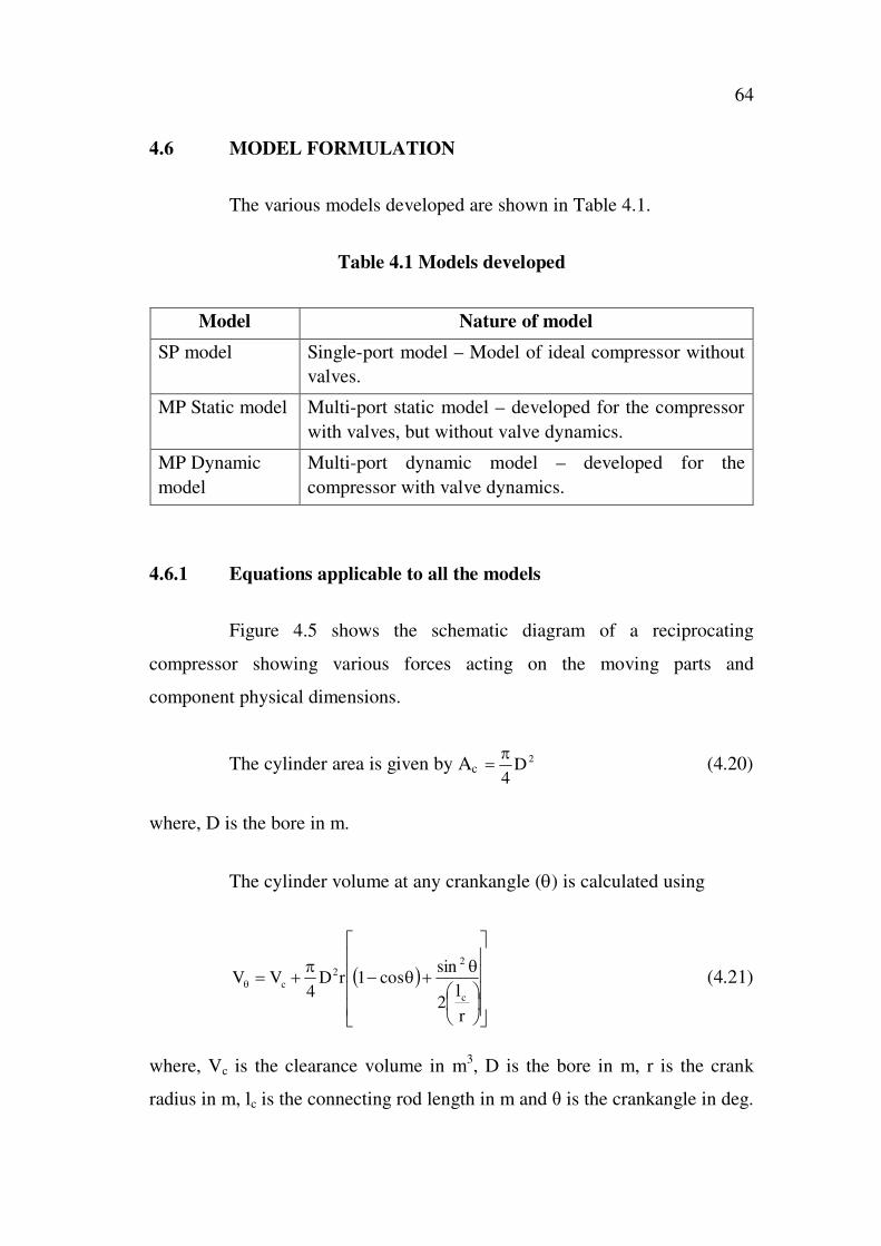
4.6 MODEL FORMULATION

The various models developed are shown in Table 4.1.

Table 4.1 Models developed

Model Nature of model

SP model Single-port model – Model of ideal compressor without

valves.

MP Static model Multi-port static model – developed for the compressor

with valves, but without valve dynamics.

MP Dynamic

model

Multi-port dynamic model – developed for the

compressor with valve dynamics.

4.6.1 Equations applicable to all the models

Figure 4.5 shows the schematic diagram of a reciprocating

compressor showing various forces acting on the moving parts and

component physical dimensions.

The cylinder area is given by Ac2D

4(4.20)

where, D is the bore in m.

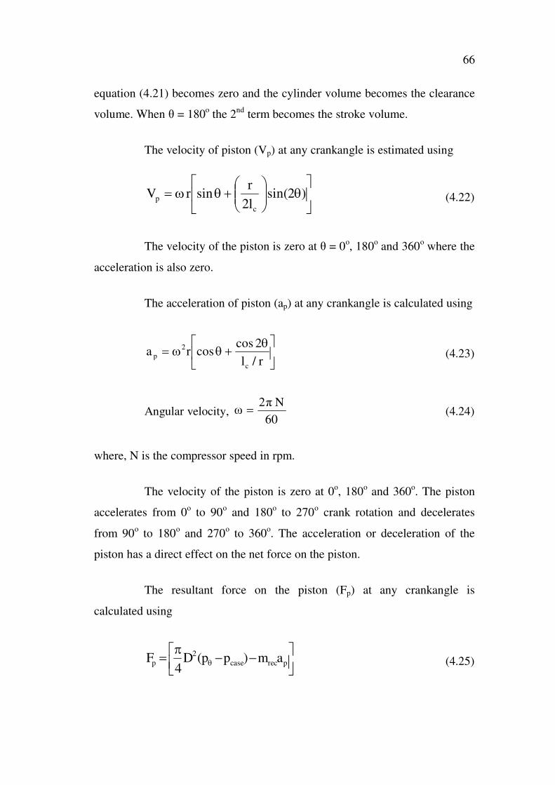
The cylinder volume at any crankangle ( ) is calculated using

r

l2

sincos1rD

4VV

c

22

c (4.21)

where, Vc is the clearance volume in m3, D is the bore in m, r is the crank

radius in m, lc is the connecting rod length in m and is the crankangle in deg.

65

BDC

TDCFp

D

Vc

lc

Fcr

Figure 4.5 Schematic diagram of reciprocating compressor showing

physical dimensions

Cylinder volume is the sum of clearance volume and swept or

stroke volume. The first term Vc in equation (4.21) is constant at all the

crankangles. The second term indicates the instantaneous cylinder volume.

The cycle of operation is completed in 360o crank rotation. When the piston

moves from TDC (Top Dead Centre) towards BDC (Bottom Dead Centre),

the position of the TDC is assigned a crankangle of 0o and BDC is assigned a

value of 180o. When the piston moves from BDC towards TDC, the BDC is

assigned 180o and TDC is assigned 360

o. When = 0

o or 360

o the 2

nd term in

66

equation (4.21) becomes zero and the cylinder volume becomes the clearance

volume. When = 180o the 2

nd term becomes the stroke volume.

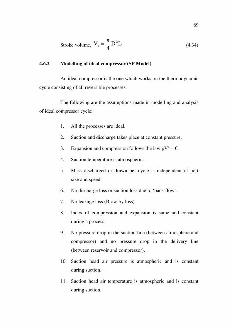
The velocity of piston (Vp) at any crankangle is estimated using

)2sin(l2

rsinrV

c

p (4.22)

The velocity of the piston is zero at = 0o, 180

o and 360

o where the

acceleration is also zero.

The acceleration of piston (ap) at any crankangle is calculated using

r/l

2coscosra

c

2

p (4.23)

Angular velocity,60

N(4.24)

where, N is the compressor speed in rpm.

The velocity of the piston is zero at 0o, 180

o and 360

o. The piston

accelerates from 0o to 90

o and 180

o to 270

o crank rotation and decelerates

from 90o to 180

o and 270

o to 360

o. The acceleration or deceleration of the

piston has a direct effect on the net force on the piston.

The resultant force on the piston (Fp) at any crankangle is

calculated using

preccase

2

p am)pp(D4

F (4.25)

67

where, p is the pressure at any crankangle in Pa, pcase is the crankcase

pressure in Pa and mrec is the mass of reciprocating parts in kg.

The resultant force on the crank (Fc) at any crankangle is calculated

using

22

c

pc

sin)r/l(2

2sinsinFF (4.26)

The resultant torque (Tr) at any crankangle is calculated using

rFT cr (4.27)

The area of port (Ao) is calculated using

2

oo d4

A (4.28)

where, do is the diameter of port in m

The density of air ( ) at any crankangle is calculated using

RT

p(4.29)

where, R is the gas constant in J/(kg.K)

The cylinder pressure (p ) at any crankangle during compression

and re-expansion is calculated using

n

11

V

Vpp (4.30)

68

where, = 0 corresponds to TDC, ( -1) denotes the previous crankangle

n = nc during compression process and n = ne during re-expansion

process

The temperature of air (Tc) at any crankangle during compression

and re-expansion is calculated using

1n

11

V

VTT (4.31)

The Free Air Delivered (FAD) by the compressor is calculated

using

a

aos

a

aod

p

RTm

p

RTm

FAD

1

4

3

2

(4.32)

where,3

2

odm is the total mass of air delivered to the reservoir in kg/s,

1

4

osm is the total mass of air inducted into the cylinder in kg/s, Ta is the

ambient temperature in K and pa is the atmospheric pressure in Pa.

The volumetric efficiency ( v) of the compressor based on mass is

calculated using

a

sa

od

v

RT

Vp

m3

2

(4.33)

69

Stroke volume, LD4

V 2

s (4.34)

4.6.2 Modelling of ideal compressor (SP Model)

An ideal compressor is the one which works on the thermodynamic

cycle consisting of all reversible processes.

The following are the assumptions made in modelling and analysis

of ideal compressor cycle:

1. All the processes are ideal.

2. Suction and discharge takes place at constant pressure.

3. Expansion and compression follows the law pVn = C.

4. Suction temperature is atmospheric.

5. Mass discharged or drawn per cycle is independent of port

size and speed.

6. No discharge loss or suction loss due to ‘back flow’.

7. No leakage loss (Blow-by loss).

8. Index of compression and expansion is same and constant

during a process.

9. No pressure drop in the suction line (between atmosphere and

compressor) and no pressure drop in the delivery line

(between reservoir and compressor).

10. Suction head air pressure is atmospheric and is constant

during suction.

11. Suction head air temperature is atmospheric and is constant

during suction.

70

12. Delivery head air pressure is equal to the discharge pressure

and is constant during discharge.

13. Delivery head air temperature is equal to the cylinder air

temperature during discharge.

14. No effect of heat transfer on index of compression and

expansion.

15. Coefficient of discharge is constant.

4.6.2.1 Suction and discharge

The pressure during suction and discharge is constant. The work

done on the air during discharge is utilised only for the removal of air from

the cylinder.

The mass of air inducted in or discharged out (mo) during is

calculated from

)VV(m 1o (4.35)

where, denotes the crankangle while -1 denotes the previous crankangle

The net mass in the cylinder during suction at any crankangle (mrs, )

is calculated from

os,1rs,rs, mmm (4.36)

The mass remaining in the cylinder during discharge at any

crankangle (mrd, ) is calculated from

od,1rd,rd, mmm (4.37)

71

The temperature of air at any crankangle (T ) is calculated from

11r,

11r,

Vpm

TmVpT (4.38)

The pressure at any crankangle (p ) is calculated from

r,

V

RTmp (4.39)

The total mass inducted in per cycle (mo) is

o,o mm (4.40)

Suction and discharge are flow processes and the indicated power

at any crankangle (IP ) is calculated using

60

NVpVpIPIP 111 (4.41)

4.6.2.2 Compression and expansion

Compression and expansion are non-flow processes and the

indicated power at any crankangle (IP ) is calculated using

60

N

1n

VpVpIPIP 11

1 (4.42)

n = nc during compression

n = ne during re-expansion

Though the equations (4.41) and (4.42) are similar, the values of p

and V are different for the non-flow and flow processes.

72

p -1

p

V -1 V

4.6.3 Development of MP static model from SP model

The suction and discharge valves are introduced in MP static

model. The model is developed with constant flow area without valve

dynamics. The maximum flow area both in suction and delivery sides is

considered. An effective model for determining the indicated power is

introduced in the model. The following assumptions have been eliminated

from the ideal compressor cycle analysis for modelling the reciprocating

compressor without valve dynamics:

1. All the processes are ideal

2. Constant pressure suction and discharge.

3. Mass discharged out or drawn in per cycle is independent of

port size and speed.

4.6.3.1 Estimation of indicated power

The area under the curve in a p-V diagram is work transfer or

indicated power transfer. Figure 4.6 shows the integration method of

determining the indicated power of the actual compressor cycle.

Figure 4.6 Integration method of determining IP

Since all the processes do not follow the particular thermodynamic

law, equations (4.41) and (4.42) cannot be used for estimating the IP. The

73

xs

general and effective model used for estimating IP during any incremental

crankangle is

60

N

2

pp)V(VIPIP 1

11 (4.43)

4.6.3.2 Suction process

The flow area is calculated assuming that the valve opens

immediately and occupies maximum effective lift. And the area is assumed to

be constant during suction. Figure 4.7 shows the plan and side views of

suction ports on the valve plate. The actual holes are shown by circles.

However for mathematical modelling the holes are assumed to be in-line as

shown by the dotted circles. Valve plate

Holes in plate

Plan view Side view

Figure 4.7 Suction port plan and side views

The maximum flow area considering only first mode of vibration isgiven by

Afs = dos Ssmax (4.44)

where, Ssmax = Maximum effective suction valve lift.

74

s

ss

maxsl

xhS (4.45)

where, xs is the distance between the centre of the port and base of the suction

valve in m.

The flow of air through the valve is considered as flow through a

nozzle. The mass of air entering the cylinder during is estimated using

ss n/)1n(

a

aa

s

sdsfsos

p

p1/p

1n

n2CAm (4.46)

where, a is the density of air at atmospheric pressure and temperature, ns is

the suction index and Cds is the suction side coefficient which is dependent on

the compressor speed and from the test results of the present work the

following empirical equation was developed for estimating Cds. The details

are given in Appendix 6.

)N00022.0N10x3N10x2.2(6.0C 28312

ds (4.47)

where, N is the speed in rpm.

The temperature of air in the cylinder at any crankangle is

calculated from

rs,

sos11rs,

m

TmTmT (4.48)

The mass of air remaining in the cylinder, the total mass of air and

the pressure of air are estimated from equations (4.36) to (4.40).

75

Stop

hSmax

l

Valve

X

Y

ValveValve

Stop

Valve PlateF

4.6.3.3 Discharge process

The discharge flow area is calculated assuming that the valve opens

immediately and occupies maximum lift. The area is assumed to be constant

during discharge. Figure 4.8 shows a reed valve in closed position and Figure

4.9 shows a reed valve in fully open position.

Figure 4.8 Reed Valve in closed position

Figure 4.9 Reed Valve in open position

The maximum flow area considering only first mode of vibration is

given by Afd = dod Sdmax (4.49)

where, Sdmax = Maximum valve lift ,d

dd

maxdl

xhS (4.50)

76

Mass of air leaving the cylinder during is estimated using

p

p1p

1n

2nCAm

dd 1)/n(n

d

d

dddfddod (4.51)

where, d is the density of air at discharge pressure and temperature, nd is the

discharge index and Cdd is the discharge side coefficient which is dependent

on the compressor speed and from the test results of the present work the

following empirical equation was developed for estimating Cdd. The details

are given in Appendix 6.

)N0002.0N10x3N10x2(65.0C 28312

dd (4.52)

where, N is the speed in rpm.

The temperature of air in the cylinder is calculated using

vrd,

2

p1pod1v1rd,

Cm

/2VTCmTCmT (4.53)

where, Vp is the velocity of piston in m/s and Cp and Cv are the specific heat at

constant pressure and constant volume respectively in J/(kg.K).

The mass remaining in the cylinder, the total mass of air and the

pressure of air are estimated using equations (4.37) to (4.40).

4.6.4 Development of MP dynamic model from MP static model

MP dynamic model is developed with valve dynamics considering

various losses and head volume. The only assumption in the MP dynamic

model is ‘expansion and compression follows the law pVn = C’. The suction

and delivery valve lifts at different crankangles are considered in the flow

77

area apart from other equations used in MP static model. The various

assumptions are relaxed in stages to study their effects on model performance.

4.6.4.1 Stage 1

In Stage 1, a simple valve dynamics concept is used to study the

behaviour of the valves. The assumptions eliminated from MP static model

are as follows.

1. No pressure drop in the suction line (between atmosphere and

compressor)

2. No pressure drop in the delivery line (between reservoir and

compressor)

The net force on the suction valve (Fs) is calculated using

soshss ZAppF (4.54)

where, phs is the pressure of air in the suction head in Pa, Aos is the suction

port area in m2 and Zs is the number of suction ports.

The initial force on the suction valve (Fsi) is calculated using

soseshssi ZAppF (4.55)

where, pes is the effective suction pressure in Pa.

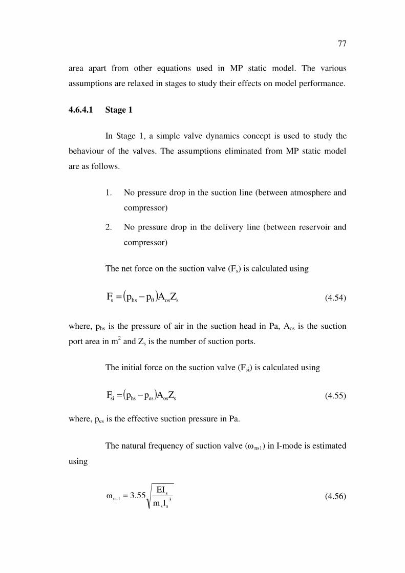
The natural frequency of suction valve ( ns1) in I-mode is estimated

using

3

ss

s1ns

lm

EI55.3 (4.56)

78

where, ms is the mass of suction valve in kg and Is is the area moment of

inertia of suction valve in m4.

The suction valve stiffness (ks) is estimated using

2

nsss mk (4.57)

Using simple valve dynamics, the suction valve lift is calculated

from

s

siss

k

FFS (4.58)

The suction flow area in the I-mode is estimated using

2

)YS(dA ss

os1fs (4.59)

where,s

ossss

x

2/dxSY (4.60)

The natural frequency of suction valve in II-mode as stated by

Francis (1965) is obtained using 3

ss

s2ns

lm

EI22 (4.61)

Suction valve stiffness and lift are calculated from Equation (4.57)

and Equation (4.58).

The suction flow area in II-mode is calculated from

Afs2 = dos (Ssmax + Ss in second mode) (4.62)

79

where, Ssmax = Maximum suction valve lift and is calculated using equation

(4.45).

The net force on the discharge valve (Fd) is calculated using

dodhdd ZAppF (4.63)

where, phd is the pressure of air in the delivery head in Pa, Aod is the area of

the discharge port in m2 and Zd is the number of discharge ports.

The initial force on the discharge valve (Fdi) is calculated using

dodhdeddi ZAppF (4.64)

where, ped is the effective discharge pressure in Pa.

The movement of the valve till it hits the valve stop is considered as

the vibration in I-mode and the movement of the valve beyond the stop is

considered as the vibration in II-mode.

Note: The II-mode of vibration in suction reed and I-mode in delivery

reed are shown in Figure 3.3.

The natural frequency of discharge valve ( nd1) in I-mode as stated

by Francis (1965) is estimated using 3

dd

d1nd

lm

EI55.3 (4.65)

where, E is the young’s modulus of valve material in N/m2, md is the mass of

discharge valve in kg and Id is the area moment of inertia of discharge valve

in m4.

80

The discharge valve stiffness (kd) is estimated using

2

nddd mk (4.66)

Using simple valve dynamics the discharge valve lift (Sd) is

estimated from

d

didd

k

FFS (4.67)

The discharge flow area in the I-mode is obtained using Figure 4.9

as

2

)YS(dA dd

od1fd (4.68)

where,d

odd

ddx

2/dxSY (4.69)

The natural frequency of discharge valve in II-mode ( nd2) as stated

by Francis (1965) is obtained from

3

dd

d2nd

lm

EI22 (4.70)

Discharge valve stiffness and lift in II-mode are calculated using

Equation (4.66) and Equation (4.67).

The discharge flow area in II-mode is estimated from

Afd2 = dod (Sdmax + Sd in second mode) (4.71)

81

where, Sdmax = Maximum valve lift and is calculated using

equation (4.50)

4.6.4.2 Stage 2

In Stage 2, the effective valve dynamics and improved flow model

are used. Backflow in suction and delivery sides is considered.

Using improved valve dynamics the suction valve lift as stated by

Piechna (1984) is estimated from

ss

vsessiss

Jk

amFFS (4.72)

where,

2

ns

22

ns

s 21J (4.73)

Fsi = Force due to initial compression of suction valve in N

mes = Equivalent mass of suction reed in kg (Details are given in

Appendix 2 and Appendix 3)

avs = Acceleration of suction reed in m/s2

= Damping factor

The air enters the port in the valve plate axially, and flows through

the gap between the reed valve and the valve plate radially. Considering the

flow through the suction reed to be a nozzle flow, equation (4.74) can be used

to estimate the mass of air drawn in through the suction reed.

The mass of air entering during incremental angle (mos) is

calculated using

82

p

p1p

1n

2nVCCAm

ss 1)/n(n

es

eses

s

s2

oasdsfsos (4.74)

Suction area correction factor is given by

c

fsc

os

fsosas

A

AA

A

AAC (4.75)

The velocity of air at the outlet of the port using continuity equation

is obtained ass

p

os

c

oZ

V

A

AV (4.76)

The loss due to back flow on the suction side is estimated using

ss

2

ossbs ZSd4

m (4.77)

The total mass drawn-in per cycle is

bsos,os mmm (4.78)

Using improved valve dynamics the delivery valve lift as stated by

Piechna (1984) is estimated by

dd

vddidd

Jk

aFFS (4.79)

where,

2

nd

22

nd

d 21J (4.80)

83

= Damping factor

Fdi = Force due to initial compression of discharge valve in N

med = Equivalent mass of discharge reed in kg (Details are given

in Appendix 2 and Appendix 3)

avd = Acceleration of discharge reed in m/s2

The mass of air discharged during an incremental angle (mod) is

calculated using

p

p1p

1n

2nVCCAm

dd 1)/n(n

d

d

d2

oadddfddod (4.81)

Discharge area correction factor is given by

c

fdc

od

fdodad

A

AA

A

AAC (4.82)

where, Ac is the cylinder cross sectional area in m2.

The flow is taking place from the cylinder through the port, valve

and head. The above correction factor increases the flow area.

The velocity of air at the outlet of the port is

d

p

od

c

oZ

V

A

AV (4.83)

The loss due to back flow is estimated using dd

2

oddbd ZSd4

m (4.84)

where, d is the density of air during discharge process in kg/m3

Equation (4.84) is derived from, m = V

84

SdDelivery reed

Delivery reed Valve plate

The reverse flow of discharged air into the cylinder is shown in

Figure 4.10. Back flow reduces the amount of air discharged through the

delivery valve.

Figure 4.10 Back flow in reed valve

The total mass discharged per cycle is

bdod,od mmm (4.85)

4.6.4.3 Stage 3

In Stage 3 of MPD model the effect of head volume and blow-by

losses are considered.

The mass of air discharged from the suction head to the cylinder

(mohs) is estimated using

pp2CAm hsdhsohshsohs, (4.86)

where, hs is the density of air in the suction head in kg/m3, Aohs is the area of

orifice in the suction head in m2 and hs is the density of air in the suction

head in kg/m3, Cdhs is the coefficient of discharge for the port in suction head.

85

The coefficient of discharge for the port provided in the head is dependent on

head volume and diameter of port in the head. Werner Soedel (1976)

suggested the following equation to estimate the coefficient, Cdh:

)]ad(a[d/VaC 3oh2ohh1dh (4.87)

where, Vh is the volume of head, doh is the diameter of port in the head and a1,

a2 and a3 are the constants obtained from the experimental results of

refrigeration compressor. The value of a1 varies from 0.008 to 0.02, a2 from

0.45 to 0.55 and a3 from 0.0058 to 0.0064.

Therefore, the coefficient of discharge on the suction side for air

compressor is estimated as

0.0061)]d(0.513[d/V0.015C ohsohshssdh, (4.88)

The net mass in the suction head (mrhs, ) at any crankangle is given

by

os,ohs,1rhs,rhs, mmmm (4.89)

The temperature of air in the suction head (Ths, ) at any crankangle

is calculated using

rhs,

1hs,1ohs,os,1hs,1rhs,

hs,m

TmTmTmT (4.90)

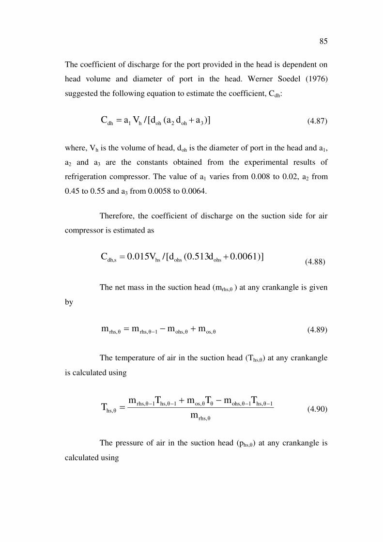
The pressure of air in the suction head (phs, ) at any crankangle is

calculated using

86

hs

hs,rhs,

hs,V

RTmp (4.91)

The mass of air discharged from the delivery head to the reservoir

(mohd ) is estimated using

pp2CAm dhddhdohdhdohd, (4.92)

where, hd is the density of air in the head in kg/m3, Aohd is the area of the

orifice in the discharge head and Cdhd is the coefficient of discharge head

which is estimated using equation (4.87) with a1 = 0.01, a2 = 0.5 and

a3 = 0.006.

0.006)]d(0.5[d/V0.01C ohdohdhdddh, (4.93)

where, Vhd is the volume of air in the discharge head in m3 and dohd is the

diameter of orifice in the discharge head in m.

The mass remaining in the discharge head (mrh, ) at any crankangle

is given by

od,ohd,1rhd,rhd, mmmm (4.94)

The temperature of air in the discharge head at any crankangle

(Thd, ) is calculated using

rhd,

1hd,1ohd,od,1hd,1rhd,

hd,m

TmTmTmT (4.95)

87

The pressure of air in the discharge head (phd, ) at any crankangle is

calculated using

hd

hd,rhd,

hd,V

RTmp (4.96)

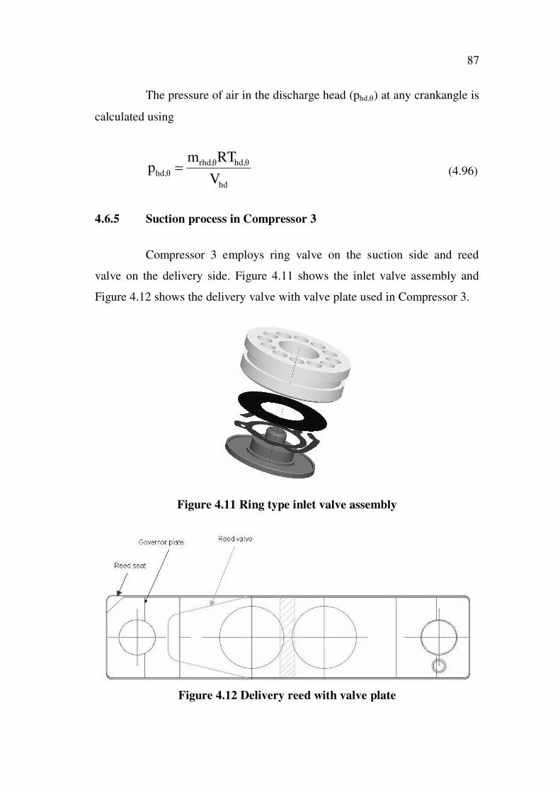
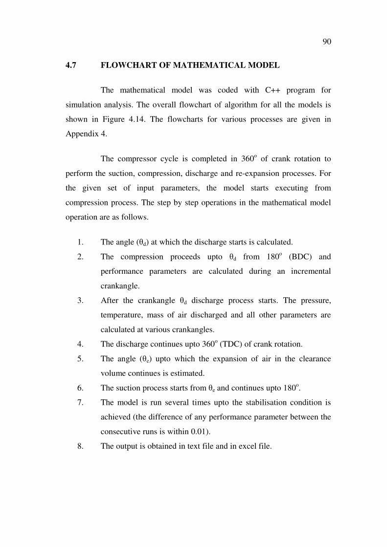
4.6.5 Suction process in Compressor 3

Compressor 3 employs ring valve on the suction side and reed

valve on the delivery side. Figure 4.11 shows the inlet valve assembly and

Figure 4.12 shows the delivery valve with valve plate used in Compressor 3.

Figure 4.11 Ring type inlet valve assembly

Figure 4.12 Delivery reed with valve plate

88

The air enters the port in the valve plate axially. Considering, the

flow through the suction valve to be an orifice flow, equation (4.97) can be

used to estimate the mass of air drawn in through the suction valve.

The mass of air entering during incremental angle (mos) iscalculated using,

)p(pVCAm hs

2

odsfsos, (4.97)

The inlet ring valve was tested for determining the stiffness (ks) at

different loads. Table 4.2 shows the stiffness of valve at different loads.

Table 4.2 Stiffness of ring valve at various loads

Load (N) Stiffness (N/mm)

0.18 0.50

0.56 0.53

0.93 0.56

1.31 0.60

1.68 0.65

2.07 0.71

2.25 0.74

An equation to determine the inlet valve stiffness has been

developed from the test results of the present work as given below. The

details are shown in Figure 4.13.

89

Figure 4.13 Variation of ring valve stiffness with load

4902.0F0429.0F0306.0k 2

s (4.97)

Using effective valve dynamics the deflection of suction valve is

estimated froms

vsssiss

k

amFFS (4.98)

4.6.6 Suction process in Compressor 4

Compressor 4 is a high speed and water cooled air compressor. It

employs ring valve on delivery and suction sides. There are 12 ports on the

suction side and 10 ports on the delivery side. The air leaves the port in the

valve plate axially. Considering the flow through the delivery valve as an

orifice flow, the mass of air leaving through the discharge port during

incremental angle is calculated using

)p(pVCAm hd

2

oddfdod, (4.99)

where, Vo is the velocity of air through the port in m/s.

90

4.7 FLOWCHART OF MATHEMATICAL MODEL

The mathematical model was coded with C++ program for

simulation analysis. The overall flowchart of algorithm for all the models is

shown in Figure 4.14. The flowcharts for various processes are given in

Appendix 4.

The compressor cycle is completed in 360o of crank rotation to

perform the suction, compression, discharge and re-expansion processes. For

the given set of input parameters, the model starts executing from

compression process. The step by step operations in the mathematical model

operation are as follows.

1. The angle ( d) at which the discharge starts is calculated.

2. The compression proceeds upto d from 180o (BDC) and

performance parameters are calculated during an incremental

crankangle.

3. After the crankangle d discharge process starts. The pressure,

temperature, mass of air discharged and all other parameters are

calculated at various crankangles.

4. The discharge continues upto 360o (TDC) of crank rotation.

5. The angle ( e) upto which the expansion of air in the clearance

volume continues is estimated.

6. The suction process starts from e and continues upto 180o.

7. The model is run several times upto the stabilisation condition is

achieved (the difference of any performance parameter between the

consecutive runs is within 0.01).

8. The output is obtained in text file and in excel file.

91

The important points to be considered while developing a

mathematical model of automotive air compressor were discussed in this

chapter. In addition, the development of actual compressor model from the

ideal model has also been explained. In Chapter 5 the details of experimental

set up with an error analysis on measured quantities are discussed.

92

Figure 4.14 Overall flowchart of mathematical model

START

Input Parameters

Calculate angle up to which expansion takes place and angle of start of delivery

Initiate the process by assigning theta=180

< d

Compression

Process

> d and

<360

Discharge Process

< e

Expansion process Suction Process= +

= +

= + = +

End

Check for stablisation

conditions

Transfer final conditions as initial

conditions

Output

<180

Yes NoNo No

92