[Type text] [Type text] 4-1

An exact Relation of the constant and periodical winds… is a part of Natural History no less desirable and useful,

than it is difficult to obtain, and its Phenomena hard to explicate

Halley, 1686

Chapter 4 Mass and Wind Fields

Overview: Radiative balance showed there must be winds to transport heat. Temperature

variations create pressure patterns. Pressure is a force initiating and sustaining the winds. Thus,

the pressure and wind patterns are intertwined. Mass and motion can be broadly explained using

simple models, including models that loop back to build further understanding of the heat

transport.

4.1 Mass Fields

4.1.1 Geopotential Height Fields Overview

The hypsometric equation (C.13) shows that the spacing between isobaric surfaces is

proportional to the temperature of the air between those surfaces. Figure 4.1 shows that the zonal

and seasonal average 1000 hPa heights, Z1000 (i.e. near sea level) have small variation compared

to the variation of higher elevation pressure surfaces. Hence, the warmer tropics have much

higher geopotential heights at 500 hPa (Z500; Figure 4.1a) than do colder higher latitudes. Though

high, the middle and upper troposphere geopotential heights are relatively flat in the tropics, as

anticipated from the similarly weak horizontal temperature gradient there (Figure 3.20). The

horizontal gradients of temperature and height are both larger in middle latitudes. This gradient

has an obvious seasonal shift with most of the gradient located from ~20-60 degrees latitude in

winter and higher latitudes in summer. The midtropospheric pressure surface heights are lower in

polar regions and lowest during winter. Thus the midlatitude Z500 gradient is strongest in winter

in both hemispheres. The seasonal shift in the latitude range of the gradient and the change in

gradient magnitude are both larger in the Northern Hemisphere. Troughs in Z1000 are found near

the equator and in middle latitudes; between is relatively higher pressure in the subtropics.

[Type text] [Type text] 4-2

Several other general comments about Figure 4.1 are as follows.

1) As anticipated in §1.2, the meridional gradient of pressure in the troposphere increases

with height.

2) Generally, the 1000hPa height has less meridional variation than isobaric surfaces for

lower pressures. The 100 hPa height field has similar shape to the 500 hPa field shown

but the amplitude is approximately twice as large (Grotjahn, 1993; Fig. 3.21).

3) The meridional pressure gradient at high altitudes is less in summer due to strong solar

heating that is rather uniform with latitude (Figure 3.6).

4) The hemispheric average surface pressure is less in the summer and greater in the winter

in both hemispheres. This indicates a net shift of mass between the two hemispheres.

5) The difference between the hemispheres is largely removed as one goes to higher

altitudes; it is almost gone by 100 hPa.

6) The Z1000 equatorial trough combined with the subtropical highs creates a low level

pressure gradient force that is opposite to the pressure gradient visible for Z500. These

gradients are consistent with Hadley circulations.

7) The Z1000 tropical trough (later located with moist convection) moves seasonally into the

summer hemisphere. Thus the Z1000 pattern is consistent with the Hadley cell being

stronger in the winter hemisphere and expanding across the equator.

8) Low pressure lies at the extratropical cyclone “storm tracks”.

4.1.2 Midlatitude Planetary Waves and Storm Tracks

As discussed in Chapter 1, the midlatitude weather is dominated by traveling frontal cyclones,

also known as extratropical cyclones. The time mean Z500 fields (Figures 4.2 and 4.3) show that

the mid and upper tropospheric pressure pattern has long waves, especially in the Northern

Hemisphere.

Also called ‘planetary waves,’ the long wave pattern in the mass fields can be anticipated

from the mid tropospheric temperature (T700) pattern shown in Chapter 3 (Figure 3.24) and

hypsometric balance. The Northern Hemisphere has main troughs near the east coasts of North

America and Asia that are associated with the cold air over Canada/Greenland and eastern

Siberia. The Asian east coast upper-level trough is not present during summer, but the eastern

North American trough remains. Presumably, the melting of the snow cover over Siberia allows

that region to warm up enough during summer. But, the Greenland and Baffin Island ice sheets

[Type text] [Type text] 4-3 inhibit this process (thus acting rather like Antarctica in the opposite hemisphere). A weaker

trough extends over the Mediterranean and Northwest Africa during DJF. Ridges are found in

between, most prominently in northwestern North America and Europe. In contrast, the time

average Southern Hemisphere height pattern tends to be rather zonal with one deep low centered

over very cold Antarctica. Southern Hemisphere time average troughs are harder to see and are

barely visible in each of the three ocean basins at 50S.

Both the Z500 and T700 fields have troughs near the east coasts of North America and Asia

during winter. Close inspection shows that the T700 trough is slightly west of the Z500 trough. The

colder temperatures at lower levels (Figure 3.23) are also over those continents but while the

1000-500hPa thickness is less there, the sea level pressure (SLP; Figure 4.4) is higher there.

Close inspection finds time mean SLP troughs to be slightly east of the Z500 troughs.

These orientations of the thermal and pressure troughs support frontal cyclogenesis. The thermal

trough upstream of the geopotential trough creates an ‘upstream tilt’ of the trough axis with

increasing elevation. How this offset of temperature and mass can amplify the mid-tropospheric

geopotential trough can be shown several ways. One way is with the so-called baroclinic

equivalent barotropic vorticity equation (or BEBVE).

The BEBVE is a variant on the vertical component vorticity equation. Cartesian

geometry is sufficient to show how the thermal trough being upstream of the geopotential trough

promotes growth of the pressure trough. The derivation is as follows (after Carlson, 1991).

Consider the quasi-geostrophic vorticity equation

gV f ft pζ ωζ∂ ∂+ ∇ + =

∂ ∂

(4.1)

Partition the geostrophic wind into two parts:

( )g B p= +gm ThV V V (4.2)

Parameter B contains all the variation of Vg with pressure. Since Vgm is the vertical average

geostrophic wind, then B=0 at the level where the geostrophic wind (Vg) equals Vgm and the

vertical (pressure) average of B is zero. This level is near 500 hPa. Thus Vgm and associated

vertical average geostrophic vertical component of vorticity, gmζ are defined as:

00 0

1

•

s sp p

s s

gm

gdp k Z dpp f p

ζ

= = ×∇

= ×

∫ ∫

∇

gm g

gm

V V

k V (4.3)

[Type text] [Type text] 4-4 The VTh wind component is a variation on the ‘thermal wind’ (shear) concept in being calculated

from the vertical average thickness field (Th). This geostrophic wind Vg can have turning when

the directions of VTh and Vgm differ. They differ when the thermal field is offset from the mass

field. Turning indicates temperature advection, but the turning is simplified by the separation of

variables placing all the vertical variation of VTh in B(p). This ‘thermal wind’ has an associated

‘thermal vorticity’. Their definitions are:

0 0

( )

sp

s

Th

g Thf p

B pζ

= ×

= • ×

∫Th

Th

V k

k V

∇

∇

(4.4)

Therefore

gm Thζ ζ ζ= + (4.5)

The equivalent barotropic vorticity equation is derived by substituting (4.2) and (4.5) into (4.1)

and integrating over the range of pressure.

0 0 0

0 0

1 1

1 1

s s s

s s

p p p

s s s

p pg Th

Th gm Th sfcs s s

fdp f dp dpp t p p p

fB dp B B f dpp t t p p

ζ ωζ

ζ ζ ζ ζ ω

∂ ∂+ ∇ + =

∂ ∂

∂ ∂+ + + ∇ + + = ∂ ∂

∫ ∫ ∫

∫ ∫

g

gm

V

V V

(4.6)

Where ωsfc is the pressure velocity at p=ps. The nonlinear terms do not have ‘cross’ products of

thermal and geostrophic components because the vertical integral of B vanishes. However the

vertical integral of B2 will not vanish. Simplifying obtains the BEBVE:

2

0

1 spgm

gm Th sfcs s

ff B dpt p p

ζζ ζ ω

∂= − ∇ + − ∇ +

∂ ∫ gm ThV V (4.7)

The B2 term is the key for the growth of the geostrophic vorticity and by extension growth of the

vertical mean geopotential trough. If the thermal trough is upstream from the geopotential

trough, then the B2 term will be positive where ζgm is positive thereby amplifying ζgm and thus the

geopotential trough at 500 hPa.

At the base (equatorward side) of each trough the height contours are more closely

spaced; from geostrophic wind balance one expects the wind speeds to be relatively stronger

there. Consistent with the zonal average distribution (Figure 4.1) the time average Z500 gradient

(Figure 4.2) is strongest in middle latitudes. While the peak gradient (the slope in figure 4.1a) is

similar all year in the Southern Hemisphere, the net change from equator to pole is smaller in the

[Type text] [Type text] 4-5 summer. In the Northern Hemisphere the net change and the gradient are both weaker during

summer.

Frontal cyclones form, propagate, and decay in specific regions. Figure 4.2 shows various

archetypal tracks followed by many frontal cyclones. The tracks are a schematic synthesis of

material presented in these sources: van Loon (1966), Whitaker and Horn (1984) ,Simmonds and

Murray (1999), Hoskins and Hodges (2002), Hoskins and Hodges (2005), and Dos Santos

Mesquita (2008). Individual tracks of cyclones vary, but the thicker dashed arrows indicate

schematically the more common paths.

Cyclogenesis is favored in three types of regions: i) near the east coasts of continents, ii)

where large-scale surface temperature gradients are strong, and iii) on the lee side of major

mountain ranges. The long wave troughs near those east coasts have stronger height gradient and

therefore stronger geostrophic winds. From simple baroclinic instability arguments, perturbations

on the flow can amplify more rapidly where the vertical shear is larger (1.5). As discussed in

Chapter 1, there are qualifiers such as the latitude and static stability. Consistent with thermal

wind shear, the stronger winds lie above stronger temperature gradients so one can base the

baroclinic instability argument on either the vertical shear or the horizontal temperature gradient.

The time mean surface temperature gradient is also strong near the east coasts of North America

and Asia due to the juxtaposition of cold land mass and oceanic WBCs. A region of stronger

meridional sea surface temperature gradient lies south of Africa and across much of the Southern

Indian Ocean. Further south, the near-surface temperature gradient is intensified at the edge of

Antarctic sea ice. Finally, simple potential vorticity arguments can explain cyclogenesis

preference downwind of mountain ranges with meridional extent.

The Ertel potential vorticity (QE) is a conserved quantity for adiabatic motion in potential

temperature coordinates (Appendix C.3); from (C.49):

gE

fQ g p

ζ

θ

+=

∂∂

(4.8)

In middle latitudes, the flow is generally westerly. Imagining a westerly flow encountering the

mountain ranges of the western North America, such a straight flow has no curvature vorticity

where it first encounters the mountains. Ascending the mountains, the spacing (i.e. ∂p) between θ

surfaces decreases thereby reducing the denominator in (4.8). To maintain a constant QE the

numerator must also decrease, by developing some anticyclonic vorticity. The flow develops an

equatorward component and as the latitude changes f decreases as well. As air crosses the ridge

line it descends on the lee side, so the θ surfaces spread apart again and the denominator

[Type text] [Type text] 4-6 increases. The absolute vorticity must increase to match, but the air is at a lower latitude than

before encountering the mountains and must have positive relative vorticity to conserve QE.

Expressed as curvature, the positive vorticity eventually turns the flow poleward. This motion

and vorticity imply a geopotential height trough. It is this trough that can be a ‘seed’ for cyclone

formation.

Frontal cyclones generally progress eastward and poleward as they evolve. These

cyclones often merge with or supplant the ‘semi-permanent’ Aleutian and Icelandic lows that are

visible in the SLP field of Figure 4.4. The storm tracks show up in the precipitation fields

(Chapter 5) as bands of heavier precipitation across the oceans in middle latitudes. Precipitation

also is enhanced where these storm tracks encounter mountain ranges of northwestern North

America, the southern Andes, and Western Europe.

Close inspection of Figure 4.2 shows the Northern Hemisphere storm tracks tend to lie

just east (downstream) of the time average troughs. The analysis above provides a simple

explanation to maintain the time average Z500 troughs. To understand the extratropical storm

track location requires a few more concepts. First, the baroclinic instability theory (of Chapter 1)

finds greater instability where the wind shear is greater. One may estimate the vertical wind

shear from gradient winds and by assuming the time average flow is much stronger at 500hPa

than near the surface. The southeastern sides of these troughs have the greater vertical shear and

thus more baroclinic instability. Second, it takes time for frontal cyclones to grow to appreciable

size by this mechanism and they are swept downstream as they grow. Third, as will be shown

later, these baroclinic eddies grow by transporting heat from warmer to colder regions and vice

versa. This transport occurs by warm advection ‘ahead of’ and cold air advection ‘behind’ the

lower troposphere trough. The trough in the thermal field must be offset from the pressure trough

to have temperature advection. Fourth, the trough axis develops a tilt compatible with these

temperature advections. The time mean Z500 trough is built in part by lower thicknesses created

by the time mean cold air below that level (applying the hypsometric equation). While the Z500

trough will be centered closer to the cold air than the developing surface low, it will remain

ahead of the colder air and grow mainly by the BEBVE mechanism. It would be a mistake to

assume the upper and lower troughs begin with upstream tilt. Instead, prior to cyclogenesis, the

upper and lower troughs typically are vertical and have little or no upstream tilt with elevation.

Thus, when an upper level trough comes into proximity with a surface trough, they interact and

cyclogenesis develops upstream tilt of the trough axis in the vertical (Grotjahn and Tribbia, 1995;

Grotjahn, 1996). This tilt is evident when comparing the troughs near the east coasts of North

[Type text] [Type text] 4-7 America and Asia in Figures 4.2 and 4.4. The SLP trough is east of the Z500 trough in both

places. Similarly, ahead of the lower troposphere trough, the warm air advection builds thickness

and thus builds an upper level ridge in Z500. Classic works link surface cyclogenesis to upper

level positive vorticity advection (e.g. Sutcliffe, 1947) and or temperature advection (e.g.

Petterssen, 1956).

Figures like 4.2 are static images of the time mean patterns, however weather systems

travel and the pressure pattern oscillates. The storm tracks like those shown in Figure 4.2 can be

obtained several ways and tend to fall into two groups: direct techniques that track individual

centers and proxy techniques that track frontal cyclone quantities. Proxy techniques include band

pass time filtering of height or meridional wind (e.g. Hoskins et al., 1989; Blackmon et al.,

1977), tracking deviations from a zonal average, and energetic quantities (e.g. Cai et al., 2006,

review). Direct techniques include tracking pressure centers (e.g. Whitaker and Horn, 1984),

tracking Laplacian of SLP centers (e.g. Simmonds and Murray,1999; Sinclair, 1997), and using

closed contours (Wernli and Schwierz, 2006). These techniques vary in complexity and have

different advantages and disadvantages. For example, vorticity is a better estimator of cyclone

strength since large pressure falls may arise mainly by the system tracking over a region of

generally lower pressures (e.g. Sanders and Gyakum, 1980). However, vorticity tends to be very

‘noisy’ with multiple centers associated with a single low pressure center. The storm tracks have

fascinating details (such as the midwinter suppression of the North Pacific storm track, e.g.

Nakamura et al., 2004) mainly collected in Chapter 10. Reviews include Chang et al. (2002) and

Shaw et al. (2016).

An easily calculated indirect storm track metric, square root of the time variance

geopotential ( )' 'RMS Z is shaded in Figure 4.3. Several of the metrics listed here, including that

in Figure 4.3, have the drawback of emphasizing the later stages in the frontal cyclone life-cycle

because they are proportional to the amplitude of the storm and missing the early, small

amplitude period of cyclone development. Hence, maximum values are located downstream

from the long wave troughs.

Four general features are seen the zonal average time variances of Figure 4.3b,d. This

figure uses more recent reanalysis data to update a similar figure by van Loon (1973, reproduced

in Grotjahn, 1993).

1) The variability is greater in midlatitudes than in the tropics. The pressure

variations are small in the tropics (Figure 4.2) as is the time mean variance

(Figures 4.3b,d) because the temperature variations are small there. The

[Type text] [Type text] 4-8

( )' '1000RMS Z has similar variation as SLP variance; the increase of sea level

pressure variance with latitude has been known for a long time; van Loon cites

Lockyer (1910) and Köppen (1882).

2) The activity is highest during winter, but the seasonal change of the peak values is

generally smaller in the Southern Hemisphere. The frontal cyclones gain much of

their energy from baroclinic energy conversions that are proportional to the

horizontal temperature gradient. The horizontal temperature gradient decreases

more from winter to summer in the Northern Hemisphere than in the Southern

Hemisphere (recall Figure 3.22).

3) The maximum values of variance are centered near 62N and 58S during winter.

These locations are poleward of the locations in van Loon. These locations fit the

characteristic of frontal cyclones progressing eastward and poleward. At the storm

track end, semi-permanent “cut-off” lows are sometimes developed and

sometimes the tracks merge with these deep lows. In the Northern Hemisphere,

the tracks often terminate near the Aleutian and Iceland islands leading to the

maximum variance between 50 to 60N. In the Southern Hemisphere there are

maxima near 50 to 60S. These data do not show another maximum van Loon

found near 75°S.

4) The larger values of variance are spread out more broadly in latitude in the

Northern Hemisphere. The greater spread reflects the greater meandering of the

storms as they follow the persistent long wave pattern. In contrast, the Southern

Hemisphere storms tend to track along a latitude circle more closely, especially

during summer (Figure 4.2b).

4.1.3 Sea Level Pressure, Subtropical Highs, and Hadley Cells

Near surface pressure maps showing much of the globe were produced in the late 1800’s (e.g.,

Buchan, 1889). Figure 4.4 shows the global sea level pressure pattern during seasons of 3-month

length. The equatorial trough is weak and quite longitudinally variable. In the subtropics, the

lowest pressures are over land areas during the summer. SLP over southern Asia during JJA is

especially low. The time-mean pattern over subtropical oceans is dominated by large

anticyclonic gyres. In midlatitudes the pressure is relatively higher or lower between ocean and

[Type text] [Type text] 4-9 continent, depending on season. Some areas have persistent low pressure, the main example

being off the Antarctic coastline.

Figure 4.4 shows a striking reversal of the near-surface pressure pattern from winter to

summer in the Northern Hemisphere. During winter there are deep lows centered over the north

Atlantic and north Pacific (the Icelandic and Aleutian lows) with high pressure over the

continents (the Siberian and Canadian highs). The Northern Hemisphere subtropical highs are

comparatively weak during winter. The summer pattern is the reverse of this; the subtropical

highs have expanded in area over the oceans and the pressure is lower over the land. The

Aleutian low has all but disappeared (in the summertime mean), while the Icelandic low has

shrunk and is centered over Baffin Island. The pressure pattern over the land can be explained as

a surface thermal effect. Pressure at any level is the weight of the air above that point. In winter

the cold surface air is denser; in summer the warm air is less dense compared to the nearby

ocean. The hypsometric equation also makes that colder air less thick than warmer air so the cold

high is shallow. Similar reasoning explains how the hot low is also shallow. The shallowness is

evident by comparison to Figure 4.3. The opposite pressure pattern prevails in the mid and upper

troposphere.

The Southern Hemisphere SLP pattern is different. The subtropical highs tend to be

centered over the oceans all year. The midlatitude pattern is clearly much more zonal on a time

average, with a belt of intense low-pressure cells centered near the coast of Antarctica. The

pattern explains the very low Z1000 heights remarked upon earlier (Figure 4.1). Little seasonal

change is apparent except over the continents.

A Chapter 1 ‘thought problem’ concluded that the Hadley cell was a reasonable

approximation to the zonal average circulation of the tropics. Chapter 3 temperature patterns

revealed that the Hadley cell of the winter hemisphere is stronger than of the summer

hemisphere. Geostrophic wind balance breaks down in the boundary layer and near the equator.

Thus the pressure gradient accelerates the winds ageostrophically, and recalling Ekman balance

(§1.4.2) the motion has a component from higher to lower pressure from these subtropical highs.

Synthesizing this information, it is immediately apparent that the equatorial sides of the

subtropical highs generate equatorward flow consistent with the low-level branch of each Hadley

cell (Figure 4.5). What is less apparent is why the Northern Hemisphere subtropical highs are

stronger in summer when the Hadley cell is stronger in winter. Close inspection of Figures 4.4 or

4.5 resolves this seeming contradiction. The strength of the subtropical high as measured by the

peak central pressure is not an infallible indicator of the meridional gradient from that high in the

[Type text] [Type text] 4-10 deep tropics. To wit: around 10N, the SLP gradient and meridional component of the near-

surface winds are stronger in DJF than in JJA in the Indian, western and central Pacific, and

Atlantic oceans as well as over Africa (Figure 4.5). The two Northern Hemisphere subtropical

highs are stronger in summer (over the oceans) because there is less frontal cyclone intensity in

the oceanic storm tracks. The frontal cyclones suppress the subtropical highs over a seasonal

average. However, the winter continental high in central Asia is much stronger than any

subtropical high during summer, consistent with the stronger Hadley cell. Specifically, one might

argue this consistency from Figure 4.5 at longitudes 100E-120E.

In the Southern Hemisphere, the conundrum largely vanishes. Southern Hemisphere

subtropical highs have quite different seasonal change than the Northern Hemisphere (Grotjahn,

2004; Grotjahn and Osman, 2007). The Indian and South Atlantic subtropical highs are strongest

during winter (JJA) while the South Pacific subtropical high is strongest during spring. Figure

4.5, around 10S, shows the stronger SLP gradient and equatorward winds during winter over the

Atlantic Ocean and the Indian Ocean across most of the Pacific.

The midlatitude, zonal average troughs result from preferred tracks by frontal cyclones.

A prominent difference between hemispheres is the Southern Hemisphere zonal average trough

is much deeper than in the Northern Hemisphere. This difference arises from the different

amounts of land masses shown in Figure 1.2 and the orientation of the frontal cyclone storm

tracks seen in Figure 4.2. The land mass differences are evident in Figure 4.4. The continental

regions tend to have higher sea level pressure in winter and the oceans lower pressure. Therefore,

when averaging around a latitude circle there are regions of high and low pressure that partly

compensate in the Northern Hemisphere. In contrast, between 40 S and 70 S one finds SLP

contours nearly parallel to latitude circles on a time average. Further south, hugging the

Antarctic coast is chain of low pressure centers in Figure 4.4; thus, the zonal mean pressure is

very low. This minimum has been discussed before (e.g., van Loon and Shea, 1988).

The distribution of Z1000 in the tropics and subtropics can be explained by general

physical arguments. A set of simple arguments, paralleling those in Grotjahn (1993), provide a

starting place, but to understand the circulation requires additional development.

To begin, one might imagine a horizontally uniform atmosphere from 30S to 30N. The

temperature surfaces are ‘flat’ but the temperature profile is conditionally stable, meaning the

lapse rate lies between the moist (saturated) and dry (unsaturated) rates. Initially, there is no

moist convection. Imagine moist convection introduced near the equator, where a Hadley cell

circulation has upward motion. The rising air within those clouds releases latent heat that reduces

[Type text] [Type text] 4-11 the cooling by adiabatic ascent enough so the air where the convection occurs is warmed.

Technically, the latent heating increases the potential temperature of the air that feeds into local

sinking adjacent to those clouds where it is expressed as higher temperatures. In this way, the

latent heating warms the tropical atmosphere indirectly (Randall, 2015; p.172). From the

hypsometric relation, this warmer air causes high pressure aloft compared with the subtropics,

setting up an equatorward pressure gradient in the upper troposphere. This gradient would drive

upper troposphere ageostrophic motion poleward that could shift mass from the equatorial to the

subtropical regions. Since the pressure at an elevation is the weight of all the air above, the

pressure in the lower troposphere would become higher in the subtropics and lower below the

equatorial convection. Hence, a pressure gradient in the lower troposphere is set up that forces

ageostrophic motion from higher latitudes towards the equatorial thunderstorms. This picture

(illustrated in Grotjahn, 1993, figure 3.22) is tidy but does not address several key questions,

such as: Why is the Hadley circulation stronger in the winter hemisphere? How does the local

sinking compare with the far field sinking? How much of the tropics has deep convection? How

does the Hadley cell transport the heat? The first three questions are answered next, while the

last question is answered later, in §4.2.2.

Digging deeper, the concept that the latent heating, even indirectly, generates the Hadley

cell might be misleading (Emmanuel, 2000). Much of the tropical troposphere has lapse rate

similar to the pseudoadiabatic lapse rate, so one might argue that the latent heating is already in

an approximate balance with the cooling from rising motion. Hence, the moist convection creates

that environment but if latent heating was the only driver, then one might think the Hadley cell

would be stronger in the summer hemisphere since the convection is strongest there. One might

expect stronger convection in the summer hemisphere from simple arguments like the Sun being

more directly overhead, heating up land areas (or ocean surface) that feeds low-level, large scale

convergence. However, to find a strong thermal contrast and hence meridional pressure gradient

to drive the ageostrophic motion, one must look beyond the tropics of the summer hemisphere.

The winter hemisphere subtropics have a much larger contrast with the tropical temperatures

(and pressure field) than the summer hemisphere subtropics. The stronger pressure gradient

forces stronger winds, making the Hadley cell stronger in the winter hemisphere. So, the tropical

convection is indirectly maintaining conditions in the tropics while strong net radiative cooling

in the winter subtropics sustains a strong contrast with the tropics. Figure 4.6 contrasts the

summer and winter hemisphere Hadley circulations.

[Type text] [Type text] 4-12

The summer hemisphere has net radiative warming in the subtropics (Figure 3.12c,f) at

the TOA. The temperature gradient in the summer hemisphere is weak as well (Figure 3.20). The

winter hemisphere has net radiative cooling at the TOA with a strong meridional gradient. The

winter hemisphere subtropics have a strong temperature gradient, mainly from 20 degrees

latitude poleward within the figure. That high altitude cooling air is easily imagined to sink

adiabatically. The adiabatic warming by compression only partially compensates leading to net

cooling of the air (e.g. Trenberth and Smith, 2008, figure 5). In this view, the upper level

pressure gradient is created by the strong cooling within the winter hemisphere subtropics

providing the contrast with the otherwise quasi-uniform tropical conditions. This view obviously

demonstrates how the winter Hadley cell is stronger.

The simple schematic of Figure 4.6 also provides a context to introduce some additional

complexity fundamental to the Hadley cell tropical convection. The rising motion is drawn

within thunderstorms by necessity for the following reason. The distribution of moist static

energy (MSE; see appendix C) inhibits vertical motion except within the lower troposphere.

Figure 4.7a,b shows the distribution of MSE . There is a general tendency for dry static energy

(DSE) to increase towards the ICZ (due to warmer temperatures) and to increase with elevation

(due to the atmosphere being statically stable so that the gZ term dominates the CPT term). The

dotted lines in the vertical cross sections show that low level air flowing towards the ICZ is

gaining DSE. The air flowing towards the ICZ is also being moistened so MSE increases more

than DSE. Eventually, the MSE rises to values at 1000hPa that exceed corresponding MSE

values above until a level near 250hPa (~10km). In regions of preferred climatological

convergence (Figure 4.7c,d) the time mean values are another 5-10% higher (>3.4x105 m2s-2)

than the MSE values at 1000hPa. These preferred regions include: southern Amazonia, Congo

basin, Australia’s Northern Territory, and the island of Papua New Guinea during DJF; while

during JJA the regions cover Panama, Bangladesh and northeastern India, and the Philippines

(along with adjacent ocean of the so-called Pacific ‘warm pool’). So, at low levels the time mean

MSE has horizontal variation created by the wind field (convergence) and land-ocean

temperature contrasts. In the upper troposphere, the MSE pattern is much smoother.

Accordingly, above these preferred regions, the time mean MSE at 1000hPa is comparable to the

corresponding MSE at 150hPa (~16km). One can imagine that at specific times, smaller-scale

low-level moisture convergence creates even higher MSE values (approaching 3.6x105 m2s-2)

matched again only at even higher levels (e.g. 18km). As discussed in Chapter 3, these

[Type text] [Type text] 4-13 extraordinarily deep thunderstorms elevate the tropical tropopause and sustain the ‘cold trap’ that

‘freeze dries’ air entering the stratosphere. For air to move through such a great depth it must not

be substantially mixing with the lower MSE values of the environment around these clouds.

Therefore the upward motion of the Hadley cell is insulated in what Riehl and Malkus (1958)

labelled ‘hot towers’.

The insulated ‘hot towers’ cover a far smaller area than is feasible to draw in Figure 4.7.

This follows from the asymmetry of rising and sinking motion locally. Bjerknes (1938;

summarized in Randall, 2015, p. 168-170) has a brief mathematical explanation. For local mass

balance the upward mass flux within the thunderstorm cores (= ρ wc bc) must equal the

downward mass flux in the clear air (= ρ ws bs) where the b’s are the normalized fraction of area

of cloudy and sinking regions. Hence, bs+bc=1. One might estimate the sinking from a simple

balance between the vertical advection and the radiative cooling:

s Tw DΓ= (4.9)

In the middle and lower tropical troposphere, DT ~ -2K/day and Γ~5K/km giving a vertical

velocity estimate of ws ~ -400m/day. Neglecting organized downdrafts, and horizontal

temperature gradients, the temperature tendency equations in the cloud and in the sinking air

reduce to

( )cc m

T wt

∂= Γ −Γ

∂ (4.10)

( )ss d

T wt

∂= Γ −Γ

∂ (4.11)

Within the cloud, the latent heating elevates the temperature of the ambient air if the lapse rate is

conditionally unstable (Γm < Γ < Γd). This temperature change makes the air more buoyant and

fosters the rising. In the clear air, the sinking also elevates the temperature since ws<0 and Γd>Γ.

The warming in the sinking environment around the cloud thereby reduces the buoyancy of that

rising air within the cloud. For there to be the net rising of the Hadley cell, then the increase of Tc

must exceed that of Ts and

c c s s H 0b w b w w+ = > (4.12)

It is understood that all the vertical motions are time and area averages. Subtracting (4.11) from

(4.10) yields

( ) ( ) ( )c sc m s d

T Tw w

t∂ −

= Γ −Γ − Γ −Γ∂

(4.13)

[Type text] [Type text] 4-14 Using (4.12) to substitute for ws in (4.13) yields:

( ) ( ) ( ) ( )

1 1 1c s c c c H

m m d dc c c

T T w w b wt b b b

∂ −= Γ −Γ − Γ −Γ − Γ −Γ

∂ − − − (4.14)

One notes that ( ) ( ) 0m d dandΓ −Γ Γ −Γ < and ( ) 0mΓ −Γ > . Also, the updraft velocity is far

larger than the Hadley motion if it were averaged over the entire tropical region, so the wH term

in (4.14) is neglected. In order for the convection to be sustained, the left hand side must be

positive and thus the first term must be larger than the second term. Thus

( )( )

0.5 mc

d m

bΓ −Γ

<Γ −Γ

(4.15)

The smaller the bc the larger the Tc-Ts tendency. Hence a small fraction of the area will have the

deep thunderstorms. Charney (1963) arrived at a similar conclusion using scale analysis applied

to the vertical component vorticity equation to show that dry vertical motion is smaller in the

tropics than the higher latitudes and must be concentrated within ‘a narrow band’ of moist

convection. Observations show that 4-10% of the area with ICZ convection is covered by deep

convective clouds (Mace et al, 2009). Using 5 m/s as a threshold updraft speed within these hot

towers (LeMone and Zipser, 1980) estimate that updrafts covering <1% of the equatorial tropics

are sufficient to provide the Hadley Cell rising branch. Thus, local sinking causes tropical

thunderstorms to cover about ten times the area needed to sustain the Hadley cell.

4.2 Winds

4.2.1 Hadley Cell Winds

The Hadley cell discussion continues as the emphasis segues to winds while the pressure field

recedes from (but remains in) the discussion.

Halley (1686) made the earliest known large-scale chart of the general circulation winds.

Halley’s chart (reproduced in Grotjahn, 1993, figure 1.1) shows tropical surface winds over the

oceans (30S to 30N) and it corresponds well with modern charts. The time mean wind vectors at

950 hPa in Figure 4.8 illustrate the near-surface wind pattern. The arrow length is proportional to

the vector wind speed. Since vectors are added to create this figure, areas with short arrows on

the chart are not necessarily regions of light winds. For example, equally strong winds that blow

half the time from the east and half the time from the west would have zero magnitude on this

chart. However, if the wind speed and direction are approximately steady, then the vector

average used here approximates the time mean wind speed. Consequently, the figure emphasizes

the tropical latitudes over oceans where winds reliably blow in a similar direction and speed

[Type text] [Type text] 4-15 during the season. Those tropical ocean winds have been labeled ‘trade winds’ for centuries due

to their reliability for powering sailing ships. Thus, larger arrows in Figure 4.8 in part indicate

persistence of wind direction.

From angular momentum conservation considerations in Chapter 1, one expects the

equatorward motion to have a westward component. Northeasterly and Southeasterly ‘trade

winds’ are indeed visible over the tropical Pacific and Atlantic oceans.

As noted in connection with Figure 4.5, motion around the equatorial sides of the

subtropical highs feeds the low level winds of the Hadley cells. The large scale, time average

convergence is also plotted in Figure 4.8. In connection with schematic Figure 4.6, the vertical

motion is concentrated in a small fraction of the tropics. The intertropical convergence zone

(ICZ) is revealed as these quite narrow bands of low-level convergence. Even these narrow

bands are in some sense an exaggeration, as deep, troposphere-spanning convection is only

filling 4-10% of the area within these bands (Mace et al., 2009) at any one time.

Precisely-speaking, the Hadley cell is a zonal average circulation and Figure 4.8 shows a

lot of zonal variations. To simplify the discussion, ‘regional Hadley cell’ will be used to label

longitudinal portions that are consistent with the zonal mean circulation by that name. The ICZ

across the central to eastern Pacific is remarkable in its persistence in nearly the same narrow

latitude range year round. This persistence can explain the narrowness and the larger time mean

convergence values. In contrast, broader bands: across the southern Indian ocean (DJF and SON)

and the South Pacific Convergence Zone (SPCZ) have lower average convergence due to

fluctuations in where the ICZ occurs on different days. Areas of convergence over land appear

less regular than over oceans, in part due to thermodynamic differences from the oceans. So,

these time mean maps show large ICZ meridional meanders.

Geographical variations reinforce or inhibit the seasonal change at different longitudes.

The seasonal change is subtle across the central to eastern Pacific and also in the tropical

Atlantic. The eastern Pacific ICZ has little seasonal change mainly because of the persistent sea

surface temperatures (SSTs) with cold water upwelling along the equator on a time average and

the persistent sea level pressure subtropical high off South America’s west coast. The eastern

Pacific SSTs change on a longer time scale than seasonally, in part captured by the ‘El Nino –

Southern Oscillation’ net. The regional Hadley cell is more obviously stronger in winter from

Africa over the Indian Ocean and into the western Pacific. Figure 4.8 also reveals that one might

interpret the Asian summer monsoon over Southern Asia as part of regional Southern

Hemisphere Hadley cell whose ICZ is over the continent. That monsoon convergence occurs

[Type text] [Type text] 4-16 well north of the equator. Hence, the JJA cross-equator flow over the western Indian Ocean

extends over a very large range of latitudes. Finally, it is also clear that the seasonal divisions

based on 3-month averages are not symmetric as MAM differs from SON over much of the

Eastern Hemisphere.

4.2.2 Zonal Mean Meridional Circulation Perspectives

The Hadley cell is vigorous enough that it shows up when averaging meridional winds

over all longitudes and over time. As implied by our thought experiment in Chapter 1 and by the

low level winds of Figure 4.8, the Hadley cell extends into the subtropics but not beyond. Is there

a zonal and time mean meridional circulation outside the tropics?

Above the boundary layer, the local, instantaneous zonal velocity, u has comparable

magnitude to the time and zonal average zonal velocity [u]. Such is not the case for the

meridional velocity outside the tropics. The zonal mean meridional velocity, [v], has much

smaller magnitude (by a factor of 10) than typical velocities, v measured at individual stations for

two main reasons. First, the meridional wind component is approximately geostrophic at these

latitudes above the boundary layer. So, when a zonal average is taken, a large part of that average

is an integral over all longitudes of a derivative with respect to longitude of a mass field. Since

the mass field does not have discontinuities and the integral has an uninterrupted circuit around

the earth, the geostrophic portion of the meridional wind does not contribute to [v]. Thus, the

zonal mean meridional velocity is an ageostrophic wind. Second, in middle and higher latitudes,

as deduced in Chapter 1, the primary circulation consists of eddies with large flows north and

south at a given level. However, meridional wind across a latitude circle must be balanced by a

wind the opposite direction at another level or longitude otherwise mass would accumulate (or be

lost) over time. There is some mass exchange back and forth between the hemispheres

seasonally, but the associated net meridional wind is not large. Hence, [v] is small and has been

difficult to estimate outside the tropics by direct means because the observational errors and

biases have been comparable to [v]. So, some care is needed in order to answer the question

posed in this paragraph.

One solution to obtaining [v] is to approach the problem indirectly by exploiting angular

momentum (M; eqn. 1.1) conservation with some simplifying assumptions. Namely to neglect: i)

mountain torques, ii) friction, iii) any net shift of mass across a latitude circle, and iv) time

tendency of M. Dividing a meridional cross section into latitude by pressure ‘boxes’ then the flux

of M across one face of the ‘box’ equals the sum of the fluxes across the other three faces. At the

[Type text] [Type text] 4-17 highest elevation box at a pole, there is no flux from a latitude higher than the pole and none

from above p=0 leaving two remaining box sides to be determined. One uses the continuity

equation to expresses the mean meridional vertical motion [ω] in terms of the mean meridional

velocity [v]. Then the flux of M through the box bottom is expressed in terms of [v] as is the flux

of M through the side box. The key that makes this work is [vM] includes [vu] which can have a

geostrophic contribution (as discussed in Chapter 6) and the observational network of the mid

twentieth century and beyond is good enough to estimate [vu] with sufficient accuracy to obtain

a midlatitude “Ferrel” cell. Since the formula no longer contains [ω], one solves for [v]. Next, the

continuity equation obtains [ω] and the estimates for that box are complete. An adjacent box is

solved next and again, two sides of the box are known and one proceeds in this fashion filling

every box of the cross section. In practice, directly measured [v] is used in parts of the tropics

where the meridional transport by the Hadley cell is strong. Since the continuity equation is two

dimensional (2-D), so is the resulting flow, and a 2-D flow can be represented by a stream

function. The stream function, [ψ] can be obtained from the time and zonal mean meridional

wind.

[ ] [ ]0

2 pR v dpgπψ = ∫ (4.16)

where stream function represents a two-dimensional flow:

[ ] [ ]2 cos

gvr p

ψπ ϕ

∂=

∂ (4.17)

[ ] [ ]22 cos

gr

ψω

π ϕ ϕ∂−

=∂

(4.18)

This procedure gives approximate velocity magnitudes, but the resultant stream function gives a

useful picture of the circulation patterns.

Modern reanalyses process observations through an atmospheric model having higher

order balances than geostrophic. Reanalyses can produce estimates of the mean meridional cells,

though they differ with the reanalysis used (e.g. Grotjahn, 2004). Figure 4.9 shows both the

vector motion and the stream function in each of four seasons found using winds in a current

reanalysis. The stream functions calculated in this way are depicted in Figure 4.9. A constant

amount of mass flows between each pair of contours, hence more closely spaced contours

indicate faster speed. (The contour interval is not constant in this figure.) The direction of the

[Type text] [Type text] 4-18 motion is indicated by the arrows. The most obvious pattern is a three-cell circulation in each

hemisphere similar to that envisioned by Ferrel (1856; 1859; 1893).

Six general comments about the detailed structure of the mean meridional circulations in

isobaric coordinates follow.

(1) As expected, the meridional circulation is dominated by a thermally-direct Hadley

cell in the winter hemisphere. Northern Hemisphere during DJF; Southern Hemisphere during

JJA. In both cases the Hadley cell in the summer hemisphere has much less magnitude. During

the two other seasons shown, the two Hadley cells have roughly equivalent magnitude.

(2) Also expected, the latitudinal position varies seasonally as well. The winter Hadley

cell extends on the winter side to ~30° and crosses the equator with rising centered at 5 to 10°

latitude in the summer hemisphere. During MAM and SON, the ICZ is north of the equator,

consistent with the regional Hadley cell in the Atlantic and eastern Pacific (Figure 4.8).

(3) A thermally indirect Ferrel cell is seen during all seasons in both hemispheres. The

Ferrel cells have significantly weaker circulations than the Hadley cells in this depiction.

‘Thermally indirect’ means rising where temperatures are relatively colder (at higher latitudes)

with sinking where temperatures are relatively warmer (at lower latitudes) with horizontal

motion to complete the circuit; hence the opposite flow as a ‘Hadley’ cell.

(4) The Ferrel cells do not have much variation from season to season in the Southern

Hemisphere. However, in the Northern Hemisphere the Ferrel cell is strongest during winter and

nearly disappears during summer.

(5) Figure 4.9 has slight evidence of thermally direct polar cells. The polar cells are very

weak and this apparent verification of Ferrel’s three-cell hypothesis may only be fortuitous

coincidence. Some prior calculations of the mean meridional circulation have shown polar cells

(e.g. Pauluis et al., 2008), others (e.g. Kjellsson et al., 2014) have not.

(6) The lower level horizontal flow in the cells takes place in a shallow layer near the

earth’s surface (p>700 hPa) while the upper-level return flow is somewhat concentrated near the

tropopause (300 >p> 150 hPa). Hence, examining the flow at 950 hPa (Figure 4.8) or 850 hPa

and at 200 hPa (later figures) captures the horizontal flow of these cells.

As discussed in the previous section, Figure 4.9 creates the misleading impression that

the ICZ is broad zone of relatively weak rising. Instead, the upward motion is concentrated

within thunderstorms in the zone. That is not the only mistaken impression. Another problem

was very familiar to William Ferrel. Namely, how does one account for the thermally indirect

cell in midlatitudes? The “Kuo-Eliassen” equation (Chapter 9) demonstrates that indirect

[Type text] [Type text] 4-19 meridional circulations are driven by eddy fluxes and diabatic fields. For now, the picture is

better understood by looking at the mean meridional circulation using alternative vertical

coordinates.

Potential temperature (θ) is considered first, then equivalent potential temperature (θe).

An advantage of θ coordinates is that adiabatic flow is confined to isentropic surfaces (constant θ

surfaces). Theta surfaces bend upwards over cold regions and downward over hot regions.

Hence, adiabatic flow is not limited to surfaces of constant pressure or height. Diabatic processes

cause air parcels to migrate from one θ surface to another. If the only diabatic process is latent

heat release by condensation, then air parcels stay on constant θe surfaces. Time and zonal mean

seasonal distributions of both variables are shown in Figure 4.10. The patterns for these variables

are similar to those for dry and moist static energy (Figure 4.7) because the quantities are

thermodynamically similar. Potential temperature increases with elevation as expected from

large scale static stability and is greater in the stratosphere. The meridional gradient of θ is weak

in the tropics and largest in the middle latitudes. Equivalent potential temperature is strongly

influenced by moisture in the tropical, lower troposphere. As a result, surface values of θe are

comparable to values at ~300 hPa in the tropics, with a relative minimum near 650 hPa. Also, θe

values in the lower (polar regions) to upper (deep tropics) troposphere are clearly higher than θ.

The meridional gradient of θe is much larger and shifted toward lower latitudes than the

corresponding θ gradient. The differing gradient and values result in nearly vertical θe contours

in middle latitudes and negative θe lapse rate in the tropics and subtropics.

Near frontal cyclones, constant θ surfaces dip low where warm air is drawn ahead of

surface low pressure and rise high in the cold air behind the low pressure center. Since air

moving adiabatically remains on a θ surface, then the mean meridional circulation is more

clearly depicted by zonal averaging along constant θ surfaces than over p or z surfaces. Figure

4.11 schematically shows the motion of air relative to a θ surface near a developing frontal

cyclone. This figure reveals how a Ferrel cell in pressure coordinates is actually a thermally

direct cell in θ coordinates. In the cold air sector, to the west of the surface low, air is sinking as

it moves equatorward adiabatically. In the warm sector, to the east of the surface low, air is

moving poleward towards a colder air mass and will rise as does the potential temperature

surface where it resides. Crucially, the colder air parcel, while higher in z, is lower in θ

compared with the warm air parcel.

In broad terms, trajectories follow paths much like the schematic illustration in Palmén

and Newton (1969; their Figure 10.20). Palmén and Newton make a pair of simple heuristic

[Type text] [Type text] 4-20 arguments for the air mass moving equatorward becoming progressively shallower. Consider the

potential vorticity formula in isentropic coordinates (C.49). If the air parcels are restricted from

having or developing relative vorticity, then equatorward motion decreases the Coriolis

parameter and the pressure spacing between θ surfaces must decrease. The cold air becomes thin

enough so surface heating can moderate the air causing the cold front to stall or dissipate. If

parcels are turned anticyclonically by descending to the equatorward side of a surface high the

cold air layers thin even more rapidly. If the flow were to develop positive relative vorticity as f

decreases, then an eastward component develops so the equatorward progression again slows.

Only very cold and deep air masses can penetrate beyond 25 degrees latitude (Palmén and

Newton, 1969).

When the paths traced out by the warm and cold air parcels in Figure 4.10 are projected

onto the meridional plane, then the paths look like a Ferrel cell when height or pressure is the

vertical coordinate. When θ is the vertical coordinate, the parcels trace out a thermally direct

circulation shown in Figure 4.12a,b. Diabatic processes cause parcels to follow paths that

migrate to different elevations of θ seen in the figure.

(1) Since cold air (low θ) sinking behind a cold front is becoming more shallow the further

equatorward it moves, it can be more easily warmed by absorbing solar radiation, by

exchanging heat with the earth’s surface (if it is near the surface), and/or from penetrative

convection (if it is not near the surface). Hence, the low level flow has lower θ values that

increase along the path toward the equator.

(2) As frontal cyclone warm sector air parcels (middle θ values) reach a front, precipitation

forms and consequently latent heat is released. The latent heating increases θ. The result

is the paths with increasing θ in middle latitudes. The latent heat release in frontal

cyclones is most prominent in broad warm frontal cloud masses. The upward motions

near 40 degrees latitude in Figure 4.12a,b correspond well with the location of secondary

maximum (annual average) precipitation shown earlier (Figure 1.1a). Seasonal

precipitation patterns (Chapter 5) match even better.

(3) At high altitudes and most latitudes, radiational cooling is the dominant diabatic process,

causing θ to decrease.

Perhaps the most striking feature about Figure 4.12 is that the indirect, Ferrel cell is

missing. Instead of a Ferrel cell, the Hadley cell is extended further poleward by an embedded

cell circulating in the same direction. These coincident, thermally direct cells in each hemisphere

[Type text] [Type text] 4-21 seem more intuitive since they transport heat poleward as required. (They accomplish this

transport since the DSE in the poleward moving upper levels is greater than the DSE of the

equatorward moving lower levels, Figure 4.7.)

The stream function in θ coordinates can be decomposed into ageostrophic and

geostrophic components. Doing so finds an ageostrophic component primarily in the tropics and

geostrophic component primarily in middle latitudes (Townsend and Johnson, 1985).

The mean meridional cells (MMC) in isentropic coordinates can be obtained using the

transformed Eulerian mean (TEM) formulation. When the zonal component momentum equation

is zonally-averaged, the result includes both zonal mean flow and divergence of eddy momentum

fluxes. (These eddies are defined by subtracting the zonal average from each total wind

component.) The meridional and vertical motions are ‘transformed’ by adding a contribution by

the meridional heat flux; in turn these define an associated MMC stream function. The eddy

fluxes of momentum and heat are separate terms. The TEM stream function (e.g. Juckes, 2001)

in ln(p) coordinates closely resembles the MMC in θ coordinates (e.g. Townsend and Johnson,

1985). The TEM formulation yields some advantages: 1) it can reproduce the isentropic

thermally-direct circulation in isobaric coordinates and 2) the separate eddy fluxes allows their

contributions to the MMC to be isolated. One problem with the formulation is it depends on the

vertical coordinate to be monotonic. As Figure 4.10 makes clear, θe has a vertical gradient that

changes sign in the tropics and part of the subtropics.

By using a ‘statistical’ extension of the TEM formulation, Pauluis et al. (2011) calculate

the MMC in θe coordinates while still retaining the ability to separate the heat and momentum

fluxes. Figure 4.12c,d shows the circulation in θe coordinates. The meridional cell is further

simplified, revealing that indeed the rising motion near 40 degrees latitude is due to latent

heating (to the extent it can overcome cooling by radiation). Consistent with Figure 4.10, the

lower portion of the circulation is at θe values that are noticeably higher than corresponding θ

values. Paulius et al. also partitioned the heat flux into sensible and latent contributions. In so

doing, the single cell in each hemisphere is shown to have somewhat larger contribution by

sensible heat flux at higher latitudes: stream function magnitude peaking at latitudes 40-50

degrees, while latent heat flux creates a stream function peaking around latitudes 25-35 degrees.

Schematic Figure 4.11 is based on the growing stage of a frontal cyclone. During the

decaying stage, the surface and upper level low centers have migrated away from the frontal

zone. Often the surface low merges with or displaces a pre-existing ‘semi-permanent’ low. Semi-

permanent lows are the Aleutian and the Icelandic lows visible in Figure 4.4. The surface high

[Type text] [Type text] 4-22 may merge with a subtropical high. A divergent circulation can be imagined as rising near the

surface lows (in part by surface friction: Ekman pumping, Chapter 1) with sinking near

subtropical highs. This circulation is like a ‘regional’ Ferrel cell when viewed in isobaric

coordinates, at least at upper levels. This motion is a divergent circulation, so it is an order of

magnitude smaller than the geostrophic components, hence one argues that even in θ coordinates

the ‘regional’ MMC for the decay stage may be much weaker than where frontal cyclones grow

baroclinically. Also, the meridional motions in θ coordinates (e.g. Johnson, 1989; his figure 10a)

do not separate vertically during the decaying stage as they do in Figure 4.11. Finally, the

decaying stage eddies transport little sensible or latent heat (Lau, 1978) in the net compared with

the growing stage, so one expects little contribution to the MMC in θ coordinates.

As indicated, the Hadley circulation in all three coordinate frames shown is thermally

direct. That statement raises the obvious question of how does the Hadley cell transport heat?

Figure 3.18 suggests that the net (vertical and zonal average) heat flux is a smaller difference

between two larger quantities of opposite sign. There is a net heat transport poleward even

though there is no net transport of mass because the potential temperature increases with

elevation (i.e. the atmosphere is statically stable). Similarly, DSE (Figure 4.10) is larger at higher

than lower elevations, leading to a net sensible heat flux.

The vertical and zonal average sensible heat flux was discussed in §3.2.2. The formula

(3.17) can be used to obtain the atmospheric sensible heat flux (ASHF) across a latitude φ within

an atmospheric layer Δp thick.

[ ] ( ) 1[ ] 2 cosASHF DSE v r g pπ ϕ −= ∆ (4.19)

where the vertical integral over pressure has been approximated using vertical average values for

the layer. From values of [v], one can estimate the net atmospheric sensible heat flux and

compare it with observed values. To make a comparison, the transport across 20 N is assumed to

occur in an atmospheric column encircling the earth that is divided into northward and southward

flowing layers. The meridional flow must have no net transport so [v] = +1 m/s in a layer from

100-400 hPa while the lower layer has stronger [v] = -2 m/s, but is proportionally thinner: 850-

1000hPa. From Figure 4.7, a reasonable annual average value for the dry static energy (using

upper tropospheric values at 20 N) is DSE 3.5 × 105 J/kg and DSE 3.3 × 105 J/kg for the

lower layer. These values imply heat fluxes of +4.0 × 1016 W in the upper layer and -3.8 × 1016

W in the lower layer. The net transport in this simple model is close to the observed values. The

observed annual sensible heat transport in the subtropics is about ASHF = 2.5 × 1015 W (Newton,

[Type text] [Type text] 4-23 1972). Thus, only a small amount of the energy being transported at upper and lower levels

(~6%) is transported in the net across latitude φ and therefore goes into reducing the pole to

equator gradient. In a related way, it will be shown later (Chapter 7) that only a small amount

(0.1 to 0.2%) of the potential energy present in the atmosphere is used to drive the general

circulation.

4.2.2 Zonal Mean Zonal Wind

The uneven distribution of radiation sets up an uneven distribution of temperature; the

primary variation of both quantities is a meridional gradient. From simple dynamics, the

temperature gradient is proportional to wind shear in the orthogonal horizontal direction. Hence

thermal wind shear means the general circulation in the middle and upper troposphere is

dominated by westerly wind.

Figure 4.13 shows the time and zonal mean zonal wind, u fields for the extreme

seasons. Winds blowing from west to east are u >0. Negative values (winds from east to west)

are shaded. Thermal wind shear (westerly wind shear proportional to negative meridional

temperature gradient) is also evident with the included zonal and time average potential

temperature θ contours. The general pattern of u is described as follows.

Figure 4.13 creates the subjective impression of approximately no net torque applied to

the Earth as the area of tropical and Antarctic surface easterlies (shaded) is comparable to the

area of surface westerlies. High SLP resides over Antarctica (Figures 4.1 and 4.4) causing

easterlies there. Equatorward motion in Hadley cells develops easterlies from angular momentum

conservation as anticipated in Chapter 1. The latitude scale of Figure 4.13 exaggerates the area

occupied by high latitudes and true angular momentum balance for the Earth also depends on the

zonal wind speed (and other factors) but to first order there is approximate balance.

Easterly winds (shaded) occur through the depth of the troposphere in most of the tropical

latitudes and in the summer hemisphere stratosphere. A relative speed maximum of easterly wind

occurs in the winter hemisphere lower troposphere this extremum is related to the winter

hemisphere Hadley cell. The stronger Hadley cell has stronger meridional motion and thus

stronger easterly component. During JJA, another easterly speed maximum occurs in the upper

troposphere and it will be shown related to an easterly jet stream over the Indian Ocean. Easterly

winds are strongest in the stratosphere during summer.

[Type text] [Type text] 4-24 Westerly winds reach several maxima. Each westerly wind maximum in the middle

latitudes of each hemisphere at tropopause level near 200 hPa is a ‘subtropical jet’ stream in the

winter hemisphere. These subtropical jets clearly lie above the stronger meridional gradient of

potential temperature. Above the subtropical jets the θ gradient reverses sign in the lower

stratosphere which reverses the vertical shear. The subtropical jets lie at the HCBE boundary

(between the Hadley and Ferrel cells of Figure 4.9). Thus, subtropical jet locations visible in

Figure 4.13 are ~30N during DJF, ~30S and ~45N during JJA. In the summer hemisphere a jet

lies near the tropopause, but close inspection of Figures 4.9 and 4.13 reveals the summer jet is

poleward of the HCBE. Since the summer jet lies in the Ferrel cell, and the Ferrel cell is created

by eddy fluxes and diabatic processes, this jet is sometimes called an ‘eddy-driven’ jet (e.g. Lee

and Kim, 2003) or a merged jet (a merger of subtropical and eddy-driven jets, e.g. Lachmy and

Harnik, 2014). The so-called eddy-driven jet has been called the ‘polar front’ jet (e.g. Palmén,

1951; Palmén and Newton, 1969) for many decades. Polar front jets are visible in Figure 4.13:

during DJF ~50S and JJA ~70N and ~50S (the latter for p≥450hPa elevation). Notably, the polar

front (or eddy-driven or merged) jet occurs year round; its horizontal fluctuations make it less

visible in wintertime and zonal averages. (Arguably, the DJF jet in Figure 4.13 near 30N may

have contributions from the ‘merged’ subtropical and polar front jets.) At the highest elevations

shown, a polar night jet is found in each winter hemisphere (most easily seen ~60S in JJA at the

diagram top). The potential temperature gradient continues into the lower stratosphere beneath

each polar night jet. These jets are centered at much higher latitudes than the subtropical jets.

All these velocity maxima occur above regions where there exist strong meridional

temperature gradients, as one expects from weaker surface winds plus thermal wind shear. The

meridional temperature gradient is often stronger in the upper troposphere for the subtropical jet,

but is often stronger in the lower troposphere for the polar front jets. These temperature gradient

elevations were also well-known decades ago (e.g. Palmén and Newton). Since the polar front jet

is associated with the thermal fronts of a frontal cyclone, the jet location migrates north and

south over time and longitude so one should not expect it to be particularly strong on a time and

zonal average. In contrast, the subtropical jet is more steady in time as is the Hadley cell and can

be captured better with a time average. Also, the polar and subtropical jet streams are not always

distinct, but often merge. Since the wind is primarily geostrophic (outside of the tropics), the

strongest meridional height gradients also correlate well with the areas of maximum wind speed

(Figure 4.1a).

[Type text] [Type text] 4-25 The processes that produce these local enhancements in the temperature gradients are

different between the stratosphere and the troposphere. Photochemical processes and the

tropopause being highest in the tropics set up the stratospheric temperature gradient (Figure

3.20). The tropospheric jets arise from the mean meridional cells and the midlatitude eddies, as

detailed in Chapter 9.

Seasonal variations are complex. This stratospheric reversal of wind direction with

season could be anticipated from the zonal average temperature fields (Figure 3.20). The

seasonal variation of the subtropical jet is also noticeable. The winter jet is stronger (>40 m/s)

than the summer jet (SHem: 30m/s; NHem: >20m/s). The jet stream core moves to lower

latitudes in winter, centered at ~30° latitude in winter and ~45° in summer. As with other

variables, the seasonal variation of the Northern Hemisphere jet is greater than in the Austral

Hemisphere. However, the polar night jet has bigger seasonal change in the Southern

Hemisphere. The polar night jet is much stronger in the Southern Hemisphere, reflecting the

much colder polar, tropospheric temperatures during winter. The polar night jet is not well

identified in Figure 4.13 due to the choice of vertical axis. The location of the polar night jet

varies strongly and rapidly with the seasons; its elevation typically ranges from 35 to 60 km (5 to

0.3 hPa) during the winter months (e.g., Hartmann, 1985). During June through August 1979,

Lau (1984) finds the maximum wind speed at 50 hPa to be about 52 m/s.

If eddies try to build time mean [u] poleward of the HCBE by momentum convergence,

then the meridional flux of zonal mean absolute vorticity, opposes the change. To show this, one

can partition the wind components due to zonal average and eddies (deviations from zonal mean)

in the zonal component momentum equation (C.26) in Cartesian and isobaric coordinates:

[ ]( ) [ ]( ) [ ]( ) [ ]( ) [ ]( ) [ ]( ) [ ]( )' ' ' '' ' ' a

u u u u u u u uu u v v fv

t x y pω ω

∂ + ∂ + ∂ + ∂ ++ + + + + + =

∂ ∂ ∂ ∂

(4.20)

Here, va is defined using a variable Coriolis parameter for the geostrophic wind definition for

convenience. The continuity equation (C.30) is used to write meridional and vertical advections

in (4.20) into flux form. Applying a zonal average eliminates all eddy/zonal mean cross product

terms to obtain:

[ ] [ ] [ ] [ ] [ ] [ ]a

u u u v u u vv u f vt y p y p y p

ω ωω ∂ ∂ ∂ ′ ′ ′ ′ ′ ′ ∂ ∂ ∂ ∂′+ + + + + + = ∂ ∂ ∂ ∂ ∂ ∂ ∂

(4.21)

Assuming the divergence multiplied by the eddy zonal wind is negligible compared to other

terms and dropping the time tendency of the eddy zonal wind obtains:

[Type text] [Type text] 4-26

[ ] [ ] [ ] [ ] [ ]a

u u u v u uv ft y p y p

ωω ∂ ∂ ∂ ′ ′ ′ ′ ∂ ∂

= − − − − ∂ ∂ ∂ ∂ ∂ (4.22)

Assuming we are at jet stream level (to ignore [ω]) and at that level the vertical eddy flux is

much smaller than the horizontal (Dima et al., 2005) leaves:

[ ] [ ] [ ]a

u u v uv ft y y

∂ ∂ ′ ′ ∂= − − ∂ ∂ ∂

(4.23)

If the center of the subtropical jet is at the HCBE, then [va]=0 since that spot is at the boundary

between the Hadley and ‘Ferrel’ cells. If the jet does not change magnitude over time then the

tendency term vanishes in (4.23) and the eddy momentum flux term must be zero or negligible

and cancelled by terms neglected. Poleward of the subtropical jet, eddies are present, perhaps

eddy momentum convergence could create a local change of [u] and move the zonal average jet

axis poleward? The horizontal eddy momentum convergence (second term on the RHS of (4.23)

would be positive. But, [va]<0 there and the horizontal shear, ∂[u]/∂y<0, reinforces the Coriolis

parameter to make the first term on the RHS of (4.23) negative and oppose that change in [u]. On

either annual or seasonal averages, both terms on the RHS are larger in the upper troposphere but

nearly cancel (Dima et al., 2005). The planetary boundary layer (where the first term balances

frictional drag upon zonal momentum) could be different. The cancellation poleward of the

subtropical jet is consistent with maintaining thermal wind balance as will be shown when

discussing the ‘Kuo-Eliassen’ equation (Chapter 9).

Chapter 1 has a general discussion of baroclinic instability where the instability (and

hence the growth rate of an eddy) is proportional to the meridional temperature gradient, and

hence the zonal wind vertical shear. One might expect the strong shears of the subtropical jet to

favor eddy growth at the subtropical jet location and some linear models find that (e.g. Baines

and Frederiksen, 1978). Nonlinear idealized studies find that eddies form on an initial jet but

through their upper level momentum fluxes build a jet at a higher latitude (initially 40N,

migrating to 45N in Simmons and Hoskins (1978); initially 45N going to 50N in Grotjahn and

Lai, 1991). However, the process is a bit more subtle as static stability and the variation of the

Coriolis parameter play important roles in linear growth rates. In addition, actual frontal cyclones

can intensify fronts not just move them and cause polar front jets to curve into much higher

latitudes than the subtropical jet. And it is long known that additional frontal cyclones can

develop along these fronts (Petterssen, and Smebye, 1971; Grotjahn, 2005). In addition, Lee and

Kim (2003) show that instability and eddy growth only occurs at the subtropical jet if that jet has

sufficiently large vertical shear to overcome the stabilizing effect of the Coriolis parameter.

[Type text] [Type text] 4-27 ‘Weak’ subtropical jets (with jet core speed <50m/s for their parameter choices) have greater

linear growth rate 20-30 degrees poleward of the subtropical jet. The growth rate can be

estimated from the linear instability study of Eady (1949)

[ ]2

0.33098d ufEady growth rateestimatedzN

=

(4.24)

Furthermore eddies are able to create a zonal mean jet from an initial state that does not have a

jet (e.g. Williams, 1978).

4.2.3 Zonal Variations of Jets and Divergent Circulations

To represent the horizontal variations of the jet streams, the 200 hPa level is shown in

Figure 4.14. Zonal variations of the subtropical jet streams are linked to geopotential height and

wind patterns discussed above. Consistent with geostrophic balance, the winds are stronger

where the horizontal gradient of time mean geopotential height is stronger (Figures 4.2 and 4.3).

That gradient is often stronger at the bases of long wave troughs in geopotential (and

temperature, Figure 3.24). Jet stream relative maxima occur near the east coasts of Asia and

North America (year around), Australia and South America (during local winter), and south of

Africa (during local summer).

The NHem subtropical jet near the east coast of Asia is stronger than the corresponding

jet near North America. The largest velocities, off the east coast of Asia, average in excess of

70ms–1! These NHem maxima are much stronger during winter (DJF). The downstream end of

each of these maxima is further poleward than the upstream end. One explanation invokes how

eddies have their upper level momentum convergence stronger at later stages in their life cycle

and located both downstream and poleward of their initial latitude (Simmons and Hoskins, 1978)

and their initial latitude may have been at the subtropical jet (Blackmon et al., 1977). An

argument could be made that as a frontal cyclone pushes warm air ahead, it builds an upper level

ridge moving the thermal front (and stronger winds aloft) poleward. The lower troposphere

trough develops a poleward motion along this ridge as well. Consequently, two jets occur at

some longitudes: one considered subtropical and the other considered eddy-driven (Eichelberger

and Hartmann, 2007). On the time mean two velocity maxima occur, one south of the other, over

the eastern Pacific and the eastern Atlantic. This combination of velocity maxima contributes to

sinking above the east side of the SLP subtropical highs as will be evident when the divergent

circulation is shown and from the zonal momentum equation.

[Type text] [Type text] 4-28 The SHem jet streams are more zonally-oriented but still have a poleward bend (

southeast Pacific). In summer there is a tendency for stronger flow south of Africa. In winter

(JJA) the stronger winds occur east of Australia. The largest average velocities in the Southern

Hemisphere just exceed 50 ms–1. As anticipated from the zonal mean (Figure 4.13) there is a

secondary maximum at a higher latitude (south of New Zealand and also in the southern Indian

Ocean). The more southerly maxima are downward expressions of the stratospheric polar night

jet. The dominant jet maximum covers nearly the same longitudinal range as the weaker East

Asian jet during JJA. The similar longitudinal locations arise because these jet maxima are

linked with the areas of greatest outflow from intense near-equator convection. The match is not

coincidence and can be understood using Rossby wave source arguments (later in this chapter

section).

Zonal variations of the time mean westerly flow in the upper troposphere can be related

to ageostrophic meridional velocities. Following Namias and Clapp (1949) the zonal momentum

equation after taking a time average and neglecting vertical and meridional advection relative to

the zonal advection. Conditions are assumed as follows. i) At tropopause level where time

average vertical motion is neglected and thus the vertical advection term is neglected. ii) The

zonal variation needs to be comparable to or less than the meridional variation of u and the

advecting velocities u v> . Friction is also ignored. What remains is a simple balance between

the ageostrophic flux of planetary vorticity and the advection of zonal wind:

( ) ( )cos g auu f v f v v f v

r rϕ λ ϕ∂ ∂Φ

= − = − =∂ ∂

(4.25)

Here, vg is the geostrophic meridional wind. The geostrophic part of the Coriolis term cancels the

pressure gradient term and what remains is the ageostrophic component (vag) by definition. If one

approximates the ageostrophic wind by the divergent wind, then (4.25) indicates that poleward

ageostrophic (divergent) wind will accelerate the zonal wind downstream (to the east). Similarly,

equatorward winds are associated with deceleration of the zonal winds. Returning to the eastern

Pacific and Atlantic, the NHem jet streams have an accelerating jet equatorward of a decelerating

jet. The associated divergent flow has convergence (in the meridional plane) aloft and that

implies sinking on the eastern sides of the corresponding subtropical highs (Figure 4.4).

Divergent winds are not the same as ageostrophic winds (gradient winds differ from

geostrophic winds, for example). However, to be consistent with later figures, we approximate

the ageostrophic meridional wind with divergent wind vectors in Figure 4.14. There is some

evidence for the approximate balance of (4.25) with a poleward component of divergent wind

[Type text] [Type text] 4-29 often where there is acceleration of the time mean winds and an equatorward component of

divergent wind where there is deceleration. Exceptions occur for divergent wind, but there is

more agreement with (4.25) than not.

The full picture of the divergent flow is shown in Figure 4.15. The divergent wind

vectors reach significant magnitudes. The largest are >10 ms–1, off the east coast of Asia. More

typical maximum values are about 5 ms–1 at this pressure level. As anticipated, the poleward

ageostrophic velocities occur where the jets are increasing downstream and vice versa.

The divergent wind field is dominated by huge centers of positive and negative extrema

in velocity potential, χ. The Laplacian of velocity potential equals the divergence, hence negative

maxima of χ are areas of divergence. While the divergence is a rather noisy field, especially over

land areas (as may be estimated from Figure 4.8) inverting the Laplacian to obtain χ is a

smoothing operation that reduces greatly the short-distance variations. The prominent outflow

centers are the far western Pacific and Central America or northern South America. The north

Pacific storm track is strong and persistent enough to create its own center of time average

divergence aloft. Major convergent regions aloft overlie desert regions of the subtropics and the

subtropical oceans. The implied sinking is consistent with i) the generally clear sky and dry (and

hot) deserts as well as ii) low level stratus (Chapter 5) over adjacent oceans. Ageostrophic

convergence aloft over the eastern NHem oceans, mentioned above, is an example of this

generalization. One must be cautious about inferring MMCs from these ageostrophic motions

(Blackburn, 1985), but for a general discussion such inferences are useful. It is immediately

obvious that portions of these major divergent centers are regional Hadley cells, including being

stronger for the winter hemisphere regional Hadley cell. Judging by the meridional component at

the equator, the winter Hadley cell (southward flow) is visible at all longitudes during JJA.

During DJF most longitudes at the equator have northward flow though some small longitude

ranges do not. It is also apparent that large regions have west-east over turnings, including the

‘Walker’ cell spanning much of the equatorial Pacific.

Diverging arrows in Figure 4.15 imply rising motion below. Following the divergent

wind vectors appears to connect areas of preferred rising with the sinking. The strongest areas of

high-level divergence overlie Southeast Asia, Indonesia, and Amazonia. In northern summer, the

Walker circulation apparently connects rising motion (and thus precipitation) over the far

western Pacific with enhanced sinking over the east side of the subtropical high in the eastern

tropical Pacific. The rising air is fed by low level convergence and that results from ageostrophic

motions that occur for relatively low surface pressure (Figure 4.4). Low pass filtered

[Type text] [Type text] 4-30 observations (Grotjahn and Osman, 2007) show a correlation between heavier precipitation in

Indonesia, lower pressure there, and stronger Pacific subtropical highs

The divergent winds of the Hadley cell advect angular momentum poleward. As the

planetary contribution to M decreases, the Uamc contribution to M must increase and thereby

accelerate the flow to form the subtropical jets. The intensity of this mechanism varies

regionally. So, the prominent outflow region in the western tropical Pacific is associated with the

strongest jet streams: east coast of Asia in DJF and over Australia in JJA. The process can be

further understood by considering the “Rossby wave source” (Sardeshmukh and Hoskins, 1988).

The Rossby wave source, SR, is defined from terms in the vertical component vorticity

equation:

aa a a RD S

t ψ χζ ζ ζ ζ∂

+ ⋅∇ = − ⋅∇ − ≡∂

V V (4.26)

Here the subscript ‘ψ’ refers to the rotational part of the wind and ‘χ’ to the divergent part of the

wind. Tilting and vertical advection terms are assumed neglectable near the tropopause level. SR

equals the divergence term and the advection of absolute vorticity by the divergent winds. Since

the rotational winds contain all of the relative vorticity, the LHS of the equation moves absolute

vorticity (ζa) around but does not create ζa while the remaining terms in SR can be a source or

sink of ζa. By making this partition, one can see the effect of divergent flow upon a horizontal

stream function and the rotational flow. Larger values of rotational flow are greater than larger

values of divergent flow. Stream function is a useful depiction of the main flow patterns of the

tropics and a proxy for the mass field in the subtropics. Consequently, the rotational flow is a

proxy for the subtropical jet.

In this example, the large outflow (Figure 4.15) during DJF is centered over a region on

New Guinea and the Solomon Sea and hence, south of the equator. The outflow is associated

with a tropical maximum in precipitation that has a large net release of latent heat of

condensation. Figure 4.16 illustrates the situation schematically.

At location R: The deeper tropical thunderstorms might suggest that the stream function be

most amplified by the latent heating below. While D is largest here, SR is not large

because both the relative vorticity and the Coriolis parameter are small near the equator

and the divergent winds vanish where D peaks.

At location A: The anticyclone is maximized here. The divergence is small making the

divergence term small. But D~0 implies the divergent winds are largest here and have a

[Type text] [Type text] 4-31

northward component. The meridional gradient of planetary vorticity is positive making

SR positive and maximized.

At location T: A trough is created here near and above the cold eastern edge of Asia at

middle and high latitudes. The divergent wind tends to have a rather small meridional

component. But, the divergence is strongly negative as air sinks above the east side of

the Siberian high. Hence, SR is strongly negative and thereby reinforces a trough.

At location J: Between the midlatitude trough and the tropical anticyclone the stream

function contour spacing is compressed leading to local intensification of the

subtropical jet. Divergent winds blowing northward from the Indonesia region during

northern winter are also consistent with the acceleration of the time mean zonal wind as

illustrated by relationship (4.25). The divergent flow southward from the Indonesia

region during JJA contributes to the stronger jet over Australia by similar reasoning.

Sardeshmukh and Hoskins (1988) force a barotropic vorticity equation model with

diabatic heating centered over New Guinea with diabatic cooling centered over southeast China;

their solutions produce the stream function features observed in this region (Figure 4.17). The

lower heights to the northwest (location T) are also due to orography. Valdes and Hoskins (1989)

use a linear stationary wave model and estimate the long-wave created by orography alone to be

about 30% of the observed long-wave amplitude over East Asia. A ridge is also produced in the

opposite hemisphere during the opposite season. The diabatic heating enhances the jet stream

over Australia during their winter by building a ridge along 10 S between Africa and 170 E. The

dominance of the latent heating over Southeast Asia out to the western Pacific explains why the

winter subtropical jet is maximum at a similar longitude in both hemispheres. Sardeshmukh and

Hoskins (1988) derive an integral constraint by integrating the vorticity equation along a closed

ψ contour and applying the divergence theorem; the constraint shows that the ψ maximum must

be displaced from the χ maximum. The time evolution of the stream function is likely more

complex than the stationary pattern of Sardeshmukh and Hoskins (1988). The tropical

convection over the Indian Ocean across to the east of New Guinea can be enhanced by a low

frequency wave train emanating from Eurasia and can in turn spur a wave train back into

midlatitudes (e.g. Lau and Philips, 1986; Adames and Wallace, 2014) in addition to enhancing

the SE Asian subtropical jet. Tropical-midlatitude interactions is a major subfield of meteorology

beyond the context of this chapter; a review is presented by Stan et al. (2017).

[Type text] [Type text] 4-32 The zonal mean observations also contain a tropical easterly jet. From Figure 4.13, the

largest easterly winds are in the stratosphere. However, easterly wind maxima are identifiable at

200 hPa and are usually centered between east Africa and Indonesia (Figure 4.14) and the

maximum exceeds 20 ms–1 on a summer-long average.

4.2.4 A Simple Model Connecting Hadley Cell, Angular Momentum, and Subtropical Jet

To conclude this sub-section, a simple model is devised that can explain some gross features of

the [u] field. The description of the jet entrance region relies upon poleward ageostrophic

motion. From angular momentum conservation, poleward moving air experiences westerly

acceleration relative to the ground. The model employs angular momentum conservation,

vertically varying friction, and a Hadley cell meridional motion. The model is only intended to

show the westerly acceleration. The model is too simplistic for the Hadley cell because vertical

motions are not incorporated directly and it is assumed that the only flows are zonal average (i.e.

zonal deviations, ‘eddies’ are ignored). However, a conceptual picture of the vertical motions

could be that all parcels move up or down in thin layers at the north and south boundaries and a

fraction of the interior air parcels at each latitude sink or rise so as to maintain mass continuity.

One can write the zonal mean angular momentum per unit mass as

[ ] [ ( )]C CM R R u= Ω + (4.27)

Here, ρ is the air parcel density, Ω is the angular velocity of the earth, RC = r cos φ and r is the

earth’s radius. Ignoring mountain torques, and eddy fluxes, a conservation law for [M] becomes

[ ] [ ] 0C xd M R F

dt+ = (4.28)

Friction is modeled using a Rayleigh formulation.

x RF k u= − (4.29)

where Rayleigh coefficient, kR <0. This form of friction means that the local derivative and

frictional terms in the zonal momentum equation are related as / Ru t k u∂ ∂ = which has

exponentially decaying solutions for negative Rayleigh coefficient, kR. For illustrative purposes a

‘planetary boundary layer’ value of kR (kRb = –0.155274 days–1) is chosen for the equatorward

flow. Frictional decay in the poleward flow of our “Hadley” cell would be much less. Reasoning

by analogy with scaling arguments for Ekman layers in theoretical models (e.g., Grotjahn et al.

1995), kRf = –4.16 x 10–3 days–1 is used here.

Substituting (4.27) and (4.29) into (4.28) yields

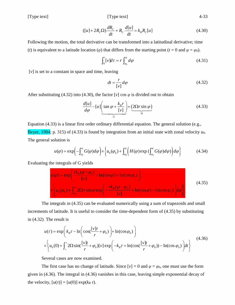
[Type text] [Type text] 4-33

[ ]([ ] 2 ) [ ]CC C R C

dR d uu R R k R udt dt

+ Ω + = (4.30)

Following the motion, the total derivative can be transformed into a latitudinal derivative; time

(t) is equivalent to a latitude location (φ) that differs from the starting point (t = 0 and φ = φ0).

00

[ ]t

v d r dϕ

ϕτ ϕ=∫ ∫ (4.31)

[v] is set to a constant in space and time, leaving

[ ]rdt dv

ϕ= (4.32)

After substituting (4.32) into (4.30), the factor [v] cos φ is divided out to obtain

( )H

G

[ ] [ ] tan 2 sin[ ]

Rk rd u u rd v

ϕ ϕϕ

− + = Ω

(4.33)

Equation (4.33) is a linear first order ordinary differential equation. The general solution (e.g.,

Beyer, 1984; p. 315) of (4.33) is found by integration from an initial state with zonal velocity u0.

The general solution is

( ) ( ) 0 0 0

0 0( ) exp ( ) ( ) ( ) exp ( ( ) )u G d u H G d dϕ ϕ ϕ

ϕ ϕ ϕϕ ϕ ϕ ϕ ϕ ϕ ϕ ϕ= − × +∫ ∫ ∫ (4.34)

Evaluating the integrals of G yields

( )

0

00

00 0 0

( )( ) exp ln(cos ) ln(cos )[ ]

( ) 2 sin exp ln(cos ) ln(cos )[ ]

R

R

rku

rku r d

vϕ

ϕ

ϕ ϕϕ ϕ ϕυ

ϕ ϕϕ ϕ ϕ ϕ ϕ

− = − +

− × + Ω − + −

∫ (4.35)

The integrals in (4.35) can be evaluated numerically using a sum of trapezoids and small

increments of latitude. It is useful to consider the time-dependent form of (4.35) by substituting

in (4.32). The result is

0

0 0

0 0 0 0

[ ]( ) exp ln cos( ) ln(cos )

[ ] [ ](0) 2 sin( )[ ] exp ln(cos( )) In(cos )

R

R

vu kr

v t v tu v k dtr r

τ

ττ τ ϕ ϕ

ϕ τ ϕ ϕ

= − + + × + Ω + − + + −

∫

(4.36)

Several cases are now examined.

The first case has no change of latitude. Since [v] = 0 and φ = φ0, one must use the form

given in (4.36). The integral in (4.36) vanishes in this case, leaving simple exponential decay of

the velocity, [u(τ)] = [u(0)] exp(kR τ).

[Type text] [Type text] 4-34 Another special case excludes friction. Either (4.35) or (4.36) may be used, but the

velocity profile is independent of time at a given latitude, so it is instructive to use (4.35). The

velocities change rapidly with latitude to compensate for the changing planetary rotational

velocity. This solution is plotted in Figure 4.18a (for poleward motion) and 4.18b (for

equatorward motion).

A more general, third case is poleward motion in the upper troposphere (using kRf and [u]

= –10 m/s at the equator). Several choices of [v] are plotted in Figure 4.18a. For slower

meridional motion, the Rayleigh friction has more time to reduce the wind speed. For the value

of kRf used here, a northward motion of 3 cm/s at 30 N results in [u] ( 35 m/s) that is close to

the observed value. But 3 cm/s is about an order of magnitude smaller than the annual and

vertical average observed [v] in the upper branch of the Hadley cell (Figure 4.9).

Equatorward flow is occurring in the surface boundary layer. Figure 4.18b (kR = kRb)

shows solutions that commence at 30 N with [u] = 10 m/s. Reasonable zonal velocities occur for

much larger meridional velocities than in the third case because friction is now much stronger.

These admittedly crude estimates of friction still allow [v] velocities that are comparable with

observed values without creating unrealistically large (negative) values of [u]. In short, if the free

atmospheric friction is increased in the simple model here, then the observed [u] and [v] profiles

in the tropics and subtropics can be reasonably matched, along with the required heat transports.

Of course this analysis also provides another simple explanation for why the subtropical

jet would lie between the Hadley and Ferrel Cells as [v] reverses sign implying not just no

further poleward advection of higher M air, but actual advection of lower M air from higher

latitudes.

However, the derivation above ignored eddy fluxes, when in fact those are large. The

equation provides a hint at more detailed discussion (Chapter 9) after a more thorough discussion

of momentum (Chapter 6). Beginning with the inviscid zonal momentum equation in Cartesian

geometry, using the continuity equation to write it in flux form, then taking time and zonal

averages yields an equation that gives a hint of things to come:

[ ][ ] [ ][ ] [ ] [ ] [ ]K L N

u v u u v uuv u f vy p y p y p

ω ωω ′ ′ ′ ′∂ ∂ ∂ ∂ ∂ ∂+ = + + + = ∂ ∂ ∂ ∂ ∂ ∂

(4.37)

The term coming from the meridional advection has a MMC part (K) as well as an eddy part (L).

Also, the vertical advection term could be further split so that term K be written as [u]∂[w]/∂p

and [ω]∂[u]/∂p where the latter part is approximately [ω]∂[θ]/∂y. Thus, the mean meridional

temperature gradient is introduced into zonal momentum discussion since the thermal wind shear

[Type text] [Type text] 4-35 relationship is a reasonable approximation at these subtropical jet latitudes. The analysis is

treated in much greater depth later, using the Kuo-Eliassen equation to show how eddy fluxes of

heat and momentum along with diabatic processes contribute to generating an MMC in the

isobaric context.

To summarize this chapter, diabatic processes and temperature patterns discussed in

Chapter 3 set up patterns of mass that have pressure gradient forces to accelerate the winds. The

winds in turn attempt to reduce the temperature gradients by transporting heat. Various

constraints reviewed in Chapter 1 along with complex variations of the surface (topography;

land, sea and ice; vegetative cover) lead to a complex circulation. However, many of the

elements anticipated in Chapter 1 ‘thought experiments’ are broadly visible in the observed

circulations. The conceptual “Hadley cell” bridges very large scale to convective scale motions:

there cannot be a broad upward-moving segment but instead a small fraction of the rapid upward

motion in tropical thunderstorms, not canceled by sinking adjacent to those storms, is the rising

branch. “Hadley cell” meridional heat transport is the smaller difference between much larger

opposite transports in upper and lower troposphere, with longitudinal variation showing both

preferential rising over specific tropical landmasses (and higher SST) and also east-west over-

turnings. Zonal wind zonal variation is linked to ageostrophic meridional winds that in turn are

linked to tropical convection plus sinking at higher latitudes. Poleward divergent motion from a

tropical source towards a midlatitude sink creates a ridge that enhances locally the jet speed. Jet

streams come in several variants, based on their driving mechanisms. Zonally-varying motions

(‘eddies’) dominate the middle and higher latitude circulation. So, eddy momentum covariances

are among the main drivers of the conceptual “Ferrel cell”. The Ferrel cell looks thermally-

indirect in pressure or elevation coordinates, but for coordinates more aligned to actual air

motions: the middle latitude circulation is thermally-direct in potential or equivalent potential

temperature coordinates. Eddies form polar front jets (among several names) while MMCs place

subtropical jets at the HCBE boundary. However, these jets organize eddies into storm tracks

wherein eddies prefer to initiate, grow to maturity, and decay. (Eddy ‘instability’ is explored

further in later chapters.) Since eddies create fronts and associated jet streams, eddies are both

influenced by the zonal mean and influencers of the zonal mean flow.

[Type text] [Type text] 4-36 Problem Sets

1. Mass of the atmosphere. a. Write down the general formula for the total amount of mass in the atmosphere for a column

with horizontal area1 m2. Calculate the mass in the column if the surface pressure is 1010hPa.

b. Write down the general formula for the total amount of mass in an atmospheric column when density is specified. (Assume a general profile of density is known, but at this point unspecified.)

c. Use your formula in part b. to estimate the mass in the unit column given surface density ρ0=1.25 kg/m3 and assuming density varies with a constant scale height based on vertical average Tave = 260K.

d. Write down the general formula for the total amount of mass in the atmosphere given surface density ρ0 and vertical average temperature Tave. Solve that formula for ρ0=1.25 kg/m3 and Tave = 255K.

e. Find the total amount of mass in the atmosphere given a surface pressure pS that is defined pS=1003(1-b cos(2φ)). Where pS is given in hPa and b=0.01.

2. Mountain torque. a. Figure 4.4d suggests a pressure difference of 8 hPa across the Andes of Chile. Deduced from

SLP values: pw=1016 hPa, pE=1008 hPa. Using the RHS of (1.2), calculate the mountain torque from φ= -π/4 to –π/3.

b. Figures 4.5d suggests the low level zonal winds are small, or 0-15 m/s. Assuming the zonal wind component at the surface is u=2 m/s and the wind speed is |V|=7 m/s, calculate the LHS of (1.2).

c. The mountain torque is what fraction of the friction? Compute your answer by taking the ratio of your answer to part a.) and divide by your answer to part b.).

3. Scale height. a. Scale heigh H is defined in Appendix B. Calculate the scale height at four these combinations

of values: (i) equator (DJF) T=300K at 1000mb. (ii) equator (DJF) 260K at 500 mb (iii) 60 N (DJF) T=260K at 1000 mb (iv) 60 N (DJF) T=238K at 500 mb. Summarize in a sentence or two how much H varies between these four locations as a percentage of the largest H found.

b. Use the average of the H values at 500 and 1000 mb to define a constant H in the isothermal formula P(z)=P(0)exp(-z/H). Find the height of the 500 mb surface at 60N and the equator for DJF.

4. MMC stream function. Calculating a stream function of a mean meridional cell based on the meridional velocity field in

the ‘tropics’. The zonal mean meridional velocity field is specified by: [vu] = Um*sin((500-P)b)*cos(L(φ-δ)) for 100 ≤ P ≤ 500 [vm] = 0 for 500 < P < 700 [vL] = Lm*cos((1000-P)a)*cos(L(φ-δ)) for 700 ≤ P ≤ 1000 Where Um = 3 m/s, Lm = -4 m/s, a = π/600 mb-1, b = π/400 mb-1, L = π/50 deg-1, δ=5 deg, P is in

mb, and φ is in degrees latitude. The subscripts U and L only indicate vertical sub-ranges of [v].

[Type text] [Type text] 4-37 a. Print out these 110 values of [v]: a 5 degree latitude interval for the latitude range from 35N to

15S gives 11 different latitudes. A 100 mb interval for pressure ranging from 100 mb to 1000 mb gives 10 vertical levels. Arrange [v] in a table with clear indications of which axis is latitude, which is pressure and such that the appropriate value of P and φ for any element of your table can be easily deduced.

b. Make a contour plot of the values of [v] for the ranges listed in part a. Be sure that your axes and contour lines are unambiguously labeled.

c. Using the indefinite integral (1.1) for each latitude and longitude, find stream function Ψ from this [v] field for the range of P and latitude in part a.

( ) [ ]

0

2 cos /P

P

r g v dPπ ϕΨ = ∫ (1.38)

P0 < P is specified vertical boundary while P is the level at which Ψ is sought. Begin by deriving the 3 general formulae for Ψ: one for each sub range of pressure levels. Then print out the 110 corresponding values of the stream function similar to what you did in part a. Arrange Ψ in a table with clear indications of which axis is latitude, which is pressure and such that the appropriate value of P and φ for any element of your table can be easily deduced.

d. Make a contour plot of the values of Ψ for the ranges listed in part a. Be sure that your axes and contour lines are unambiguously labeled.

5. Simple linkage between radiation, diabatic heating/cooling and ‘polar cell’ A glass slab calculation, diabatic cooling, compressional heating, and the motions of a “Hadley-

type” polar cell are linked in this problem. At 80 N, let aLA = 0.85, aLG = 1.0, aSA = 0.3. Assume that TG = 250 K in winter, 273 K in summer. Let TA = 225 K in winter; 240 K in summer.

a. Find IG and IA then find the IIN needed for radiative balance in each season. b. Assume the observed solar radiation absorbed at 80 N, I*, is I*=0 in winter, and I*= 171 W/m2

in summer. The difference between I* and IIN is the amount of heat flux energy needed per unit area. Call that Δ; and find that value for each season.

c. Let Δ be a loss of energy per second per square meter. What rate of heating (K/s) in the whole column is would be needed to balance this loss of energy if no work is being done? Assume that the heating rate (dT/dt) is a constant in the vertical and the surface pressure is 1.013x105 Pa. Find this heating rate for both seasons. Hints: force equals mass times acceleration, and pressure is a force per unit area. Recall the first law of thermodynamics equation: CP dT/dt = α dp/dt + DJ where DJ is a diabatic heating rate per unit mass (W/kg units). DJ is proportional to Δ. Check units for consistency.

d. The dry adiabatic lapse rate is given by g/Cp where g=9.8 m/s2 and Cp = 1004 J/(K kg). If air in the column is sinking or rising, what value of vertical velocity (w, in m/s) must be present in winter and in summer so that the local change of temperature is zero? For a bit of realism, assume that the air has lapse rate Γ = 6 K/km. Ignore any horizontal heat transport. Hints: sinking adiabatically heats the air. Also, ∂T/∂t is now zero. Check your method to ensure units are consistent.

6. Arching path from latitudinal motion. In Chapter 1, an imaginary circulation, labelled as a Hadley cell, was drawn whereby the upper

level circulation included westerly as well as poleward components. This problem is intended to examine what orientation to draw those circulations. Consider a parcel that moves from 10 N to 30 N with a constant meridional component of velocity that equals 2 m/s. Assume that friction is negligible. The parcel is initially at longitude 0 degrees and has u=U0 zonal velocity.

[Type text] [Type text] 4-38 a. Write down expressions relating meridional (y) and zonal (x) distance to longitude (λ) and

latitude (φ), respectively. From those expressions, formulate definitions of v (northward) and u (eastward) velocity using λ and φ.

b. Derive the general formula for radians of longitude travelled when proceeding from latitude φS to latitude φN The formula should not contain any unsolved integrals. Hint: use part a to convert between radians and distance and between time and space.

c. Use your formula to find the ending longitude when the parcel reaches φN = 30 N. Let the initial conditions be u=0 at 0 degrees longitude and φS = 10 N.

7. Isentropic mass weighted view versus a simple zonal average. Let a perturbation pressure field be defined as: P’ = sin(y)(1-z)cos(x) – Qzsin(x) – Syz Assume these quasi-geostrophic assumptions apply: θ’ = ∂P’/∂z v’ = ∂P’/∂x where primes denote nondimensional perturbations dimensional (total) values are given by: θ = θs ( 1 + C * θ’) P = Ps ( 1 + C * P’) v = 10 v’ ( in m/s) Z = z * 10km The subscript “s” denotes a static state (dimensional) which is isothermal with temperature

Ts =260K. The surface pressure is Ps (0) = 1.e+5 Pa. C=0.02. Q=4. S=1. And scale height H (=RTs /g) is constant.

a. Derive the formula for θs as a function of H, Ts, z and κ (where κ = R/Cp ). Ps should not be in

your final formula. Hint: Ps = Ps (0) exp(-Z/H) where if this Z is in km, then so must be H. Hint: you can check your answer: θs=265K is about 500m and θs=364 is about 9km.

b. Derive the formulae for v’ and θ’ as general functions of (x, y, z). c. Make contour plots of: P’, v’, and θ’ for z=0 and for y = (0, π) and x = (0, 2π). Do the same

for Z=9km (z =0.9). Use 21 pts in x range; 11 pts in y range. What is the value of H? These plots have P’, θ’, v’ consistent with a developing baroclinic wave and geostrophic meridional wind. Discuss: a) P’ trough location changes with height, b) where in x are: the coldest air, the upper trough, and lower trough centered, and c) which level has larger v’θ’.

d. Calculate a zonal average of v’ at (y, z) =(π/2,0.9). You may solve this numerically using the

20 grid points in the zonal direction. Trapezoidal rule is ok. You can assume that the domain is periodic. Hint: don’t double count the end point.

e. Derive the formula for the height of a potential temperature surface θo . Test out your formula

by plotting the height of the q=265K surface for x = (0, 2π) and y = (0, π). Hint: your plot should look similar to fig. 3.18 if that figure ranged from -1 to 5 km (instead of 0-10 km).

f. Plot v’ for θ=265K and θ=364K surfaces. Set the v’=0 for any point that is underground (i.e.

having elevation <0). g. Calculate 2 mass-weighted zonal averages at y=π/2 of v’: one on the q=265K surface and one

on the θ=364K. A simple mass weighting starts with the z value at each grid point of the θ surface.. Next find the Ps of each z value, next multiply the v’ value by the Ps value sum the corresponding values and call that the v’Ps sum. Next calculate the corresponding sum for the Ps values of the grid points used. Finally divide the v’Ps sum by the Ps sum. Note: Do not include any points in either sum that are underground. These upper and lower elevation mass-weighted averages will be consistent in sign with the poleward extension of a Hadley

[Type text] [Type text] 4-39

cell seen in θ coordinates. Include a labeled table of these z, Ps , and v’*Ps values for each θ surface

8. Hadley cell velocity estimates. Assume that the only MMC in the Northern Hemisphere is a large Hadley cell. The Hadley cell

has sinking occurring only from 45N to the North Pole. That sinking is given by the pressure velocity ωs = A sin(4φ) where A = -0.05 Pa/s at 800 hPa (for 45N < φ < 90N). Assume that only meridional motion occurs between 45N and 5N and all the equatorward motion at those latitudes is confined to the 800-1000 hPa layer.

a. Using the approximate formula: ω= -ρgw, estimate ws the vertical velocity of the sinking. Let ρ = 1kg/m3. Also, what is the largest value of ws?

b. What is the vertically averaged meridional velocity vH in the 1000-800 hPa layer for mass conservation at 30N? Assume the circumference of the atmosphere does not vary with elevation (but it will vary with latitude). Hint: begin by equating mass fluxes in relevant vertical and horizontal planes.

9. Hadley cell tropical thunderstorms a. Assume the following stream function vertical change during DJF at 8N: ΔΨ = 10.5x1010 kg/s

between 1000 and 850 mb elevation. Also, ΔΨ = 12.25x1010 kg/s between 300 and 150 hPa. Using formula (4.17) find [v] in each of these two layers.

b. Similar to part a, find the pressure velocity (w) in the latitude range 9-15 S given the following values of Ψ at 9S: 3.5x1010 kg/s and 15S: -1.75x1010 kg/s.

c. If the average updraft in a thunderstorm is about 500 hPa in 1 hour, find the percentage of the area between 9-15 S that is covered by thunderstorms if all the upward motion occurs in these updrafts.

d. If the average thunderstorm updraft has radius 6 km, how many thunderstorms must be present at any one time during this season?

10. Estimating the tropical easterly jet wind Estimate the jet speed over Sri Lanka during JJA from M conservation using (4.35). Assume the

starting latitude is 20N and the ending latitude is 5N. Consistent with Figure 4.14, assume [v] = -2 ms-1 over the latitude range and [u] = -10 ms-1 at 20N.

a. What is [u] at 5N if there is no friction? b. Estimate a Rayleigh friction coefficient kRf for [u] = -24 ms-1 at 5N. How does your coefficient compare with the choices in Figure 4.18a? Iterate on different values of kRf to find your answer and notice how the values alter the [u] obtained at 5N. 11. Approximating pressure gradients of a ‘Hadley’ cell This problem uses Figure 4.6 for guidance. Assume the atmosphere has constant lapse rate of 6

K km-1 and sea level value is initially 300 K at the equator and at 30S. Consider the troposphere from 200 hPa to 1010 hPa in this problem. Assume that the pressure at sea level is initially 1010 hPa at both locations.

a. Find the height of the 200 hPa surface using the Hypsometric equation. b. Assume the temperature at the equatorial sounding increases uniformly with height by 2K and

the temperature of the 30S sounding decreases uniformly by 4K. Find the new heights of 200 hPa level at the two locations. (Note. The amount of mass in each column is unchanged.)

[Type text] [Type text] 4-40 c. Assume a shift of mass occurs such that the change in 200 hPa heights is half as much as

found in part b. Based on that shift, calculate the height of the 1000 hPa surface at both locations. How does your result compare with JJA values in Figure 4.1?

d. Using hydrostatic balance and using the temperature estimated at 1000 hPa, estimate the final sea level pressure at both locations.

e. At what elevation is an isobaric surface flat?

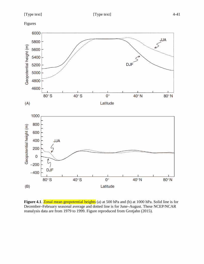
[Type text] [Type text] 4-41 Figures

Figure 4.1. Zonal mean geopotential heights (a) at 500 hPa and (b) at 1000 hPa. Solid line is for December–February seasonal average and dotted line is for June–August. These NCEP/NCAR reanalysis data are from 1979 to 1999. Figure reproduced from Grotjahn (2015).

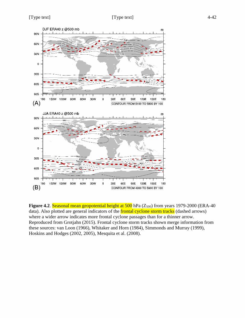
[Type text] [Type text] 4-42

Figure 4.2. Seasonal mean geopotential height at 500 hPa (Z500) from years 1979-2000 (ERA-40 data). Also plotted are general indicators of the frontal cyclone storm tracks (dashed arrows) where a wider arrow indicates more frontal cyclone passages than for a thinner arrow. Reproduced from Grotjahn (2015). Frontal cyclone storm tracks shown merge information from these sources: van Loon (1966), Whitaker and Horn (1984), Simmonds and Murray (1999), Hoskins and Hodges (2002, 2005), Mesquita et al. (2008).

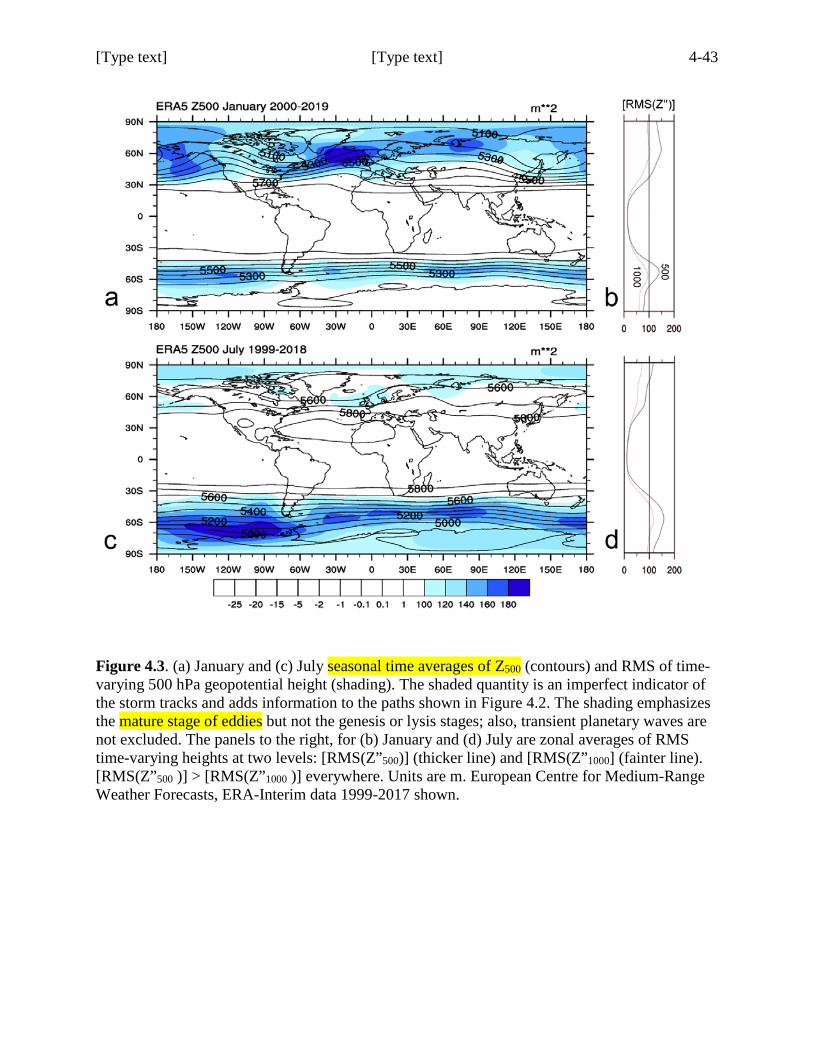
[Type text] [Type text] 4-43

Figure 4.3. (a) January and (c) July seasonal time averages of Z500 (contours) and RMS of time-varying 500 hPa geopotential height (shading). The shaded quantity is an imperfect indicator of the storm tracks and adds information to the paths shown in Figure 4.2. The shading emphasizes the mature stage of eddies but not the genesis or lysis stages; also, transient planetary waves are not excluded. The panels to the right, for (b) January and (d) July are zonal averages of RMS time-varying heights at two levels: [RMS(Z”500)] (thicker line) and [RMS(Z”1000] (fainter line). [RMS(Z”500 )] > [RMS(Z”1000 )] everywhere. Units are m. European Centre for Medium-Range Weather Forecasts, ERA-Interim data 1999-2017 shown.

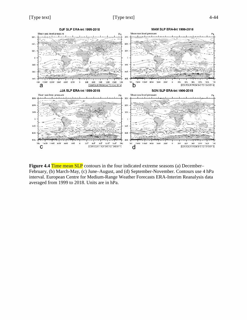
[Type text] [Type text] 4-44

Figure 4.4 Time mean SLP contours in the four indicated extreme seasons (a) December–February, (b) March-May, (c) June–August, and (d) September-November. Contours use 4 hPa interval. European Centre for Medium-Range Weather Forecasts ERA-Interim Reanalysis data averaged from 1999 to 2018. Units are in hPa.

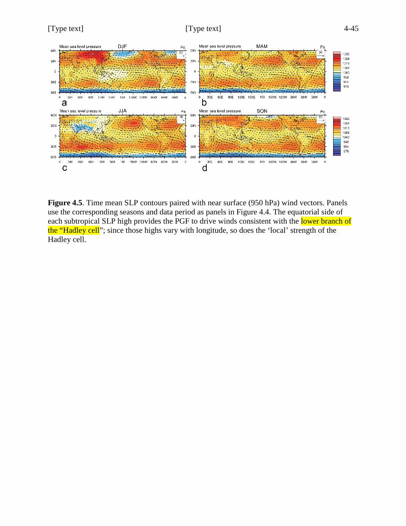
[Type text] [Type text] 4-45

Figure 4.5. Time mean SLP contours paired with near surface (950 hPa) wind vectors. Panels use the corresponding seasons and data period as panels in Figure 4.4. The equatorial side of each subtropical SLP high provides the PGF to drive winds consistent with the lower branch of the “Hadley cell”; since those highs vary with longitude, so does the ‘local’ strength of the Hadley cell.

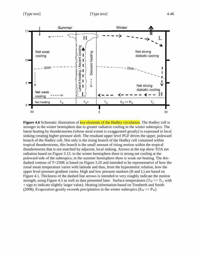
[Type text] [Type text] 4-46

Figure 4.6 Schematic illustration of key elements of the Hadley circulation. The Hadley cell is stronger in the winter hemisphere due to greater radiative cooling in the winter subtropics. The latent heating by thunderstorms (whose areal extent is exaggerated greatly) is expressed in local sinking creating higher pressure aloft. The resultant upper level PGF drives the upper, poleward branch of the Hadley cell. Not only is the rising branch of the Hadley cell contained within tropical thunderstorms, this branch is the small amount of rising motion within the tropical thunderstorms that is not matched by adjacent, local sinking. Arrows at the top show TOA net radiation based on Figure 3.12; in the winter hemisphere there is strong net cooling at the poleward side of the subtropics; in the summer hemisphere there is weak net heating. The dot-dashed contour of T=250K is based on Figure 3.20 and intended to be representative of how the zonal mean temperature varies with latitude and thus, from the hypsometric relation, how the upper level pressure gradient varies. High and low pressure markers (H and L) are based on Figure 4.1. Thickness of the dashed line arrows is intended to very roughly indicate the motion strength, using Figure 4.5 as well as data presented later. Surface temperatures (TW >> TC, with + sign to indicate slightly larger value). Heating information based on Trenberth and Smith (2008). Evaporation greatly exceeds precipitation in the winter subtropics (EW >> PW)

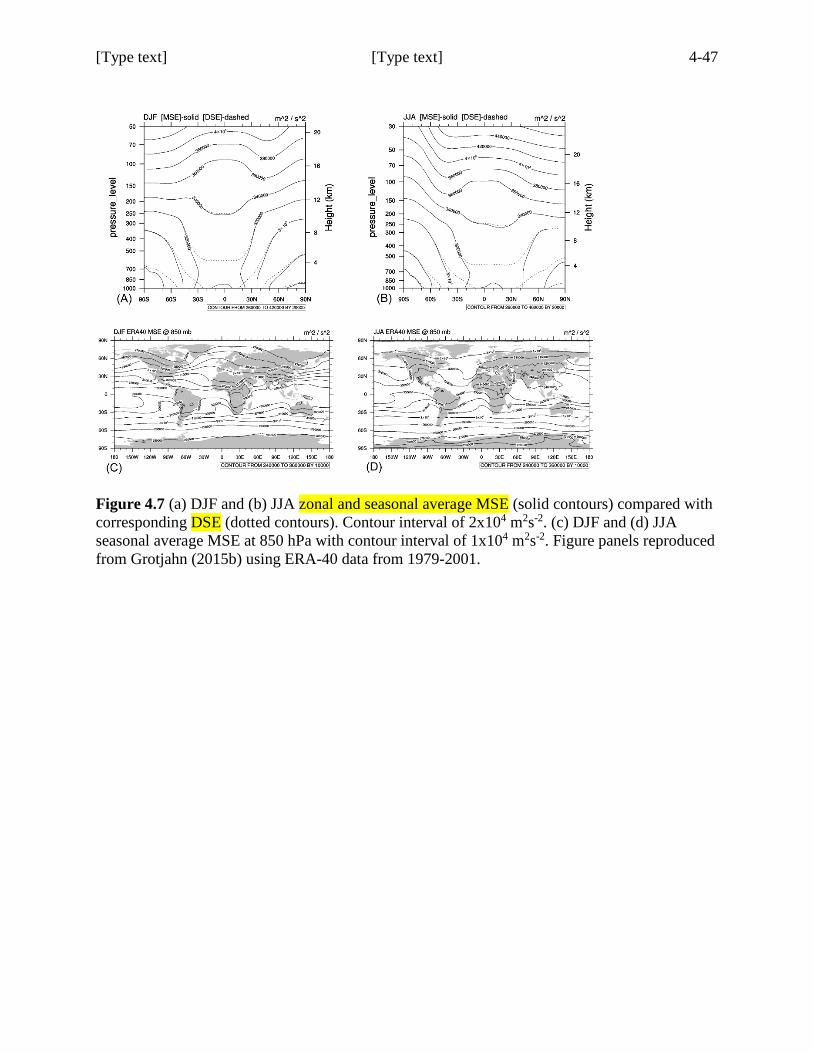
[Type text] [Type text] 4-47

Figure 4.7 (a) DJF and (b) JJA zonal and seasonal average MSE (solid contours) compared with corresponding DSE (dotted contours). Contour interval of 2x104 m2s-2. (c) DJF and (d) JJA seasonal average MSE at 850 hPa with contour interval of 1x104 m2s-2. Figure panels reproduced from Grotjahn (2015b) using ERA-40 data from 1979-2001.

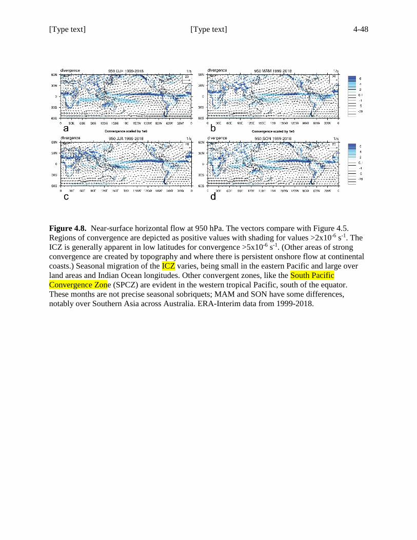
[Type text] [Type text] 4-48

Figure 4.8. Near-surface horizontal flow at 950 hPa. The vectors compare with Figure 4.5. Regions of convergence are depicted as positive values with shading for values >2x10-6 s-1. The ICZ is generally apparent in low latitudes for convergence >5x10-6 s-1. (Other areas of strong convergence are created by topography and where there is persistent onshore flow at continental coasts.) Seasonal migration of the ICZ varies, being small in the eastern Pacific and large over land areas and Indian Ocean longitudes. Other convergent zones, like the South Pacific Convergence Zone (SPCZ) are evident in the western tropical Pacific, south of the equator. These months are not precise seasonal sobriquets; MAM and SON have some differences, notably over Southern Asia across Australia. ERA-Interim data from 1999-2018.

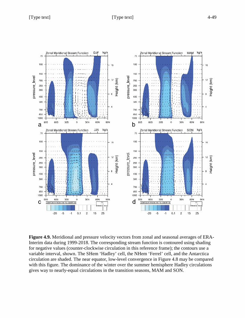
[Type text] [Type text] 4-49

Figure 4.9. Meridional and pressure velocity vectors from zonal and seasonal averages of ERA-Interim data during 1999-2018. The corresponding stream function is contoured using shading for negative values (counter-clockwise circulation in this reference frame); the contours use a variable interval, shown. The SHem ‘Hadley’ cell, the NHem ‘Ferrel’ cell, and the Antarctica circulation are shaded. The near equator, low-level convergence in Figure 4.8 may be compared with this figure. The dominance of the winter over the summer hemisphere Hadley circulations gives way to nearly-equal circulations in the transition seasons, MAM and SON.

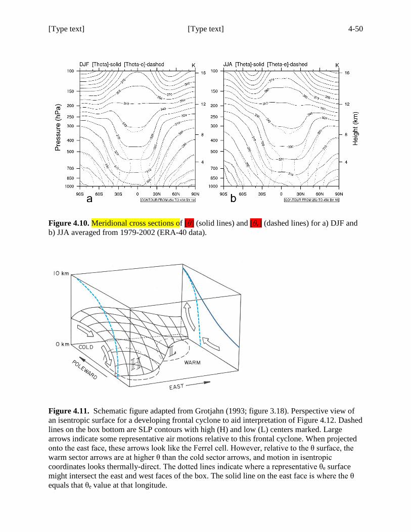
[Type text] [Type text] 4-50

Figure 4.10. Meridional cross sections of [θ] (solid lines) and [θe] (dashed lines) for a) DJF and b) JJA averaged from 1979-2002 (ERA-40 data).

Figure 4.11. Schematic figure adapted from Grotjahn (1993; figure 3.18). Perspective view of an isentropic surface for a developing frontal cyclone to aid interpretation of Figure 4.12. Dashed lines on the box bottom are SLP contours with high (H) and low (L) centers marked. Large arrows indicate some representative air motions relative to this frontal cyclone. When projected onto the east face, these arrows look like the Ferrel cell. However, relative to the θ surface, the warm sector arrows are at higher θ than the cold sector arrows, and motion in isentropic coordinates looks thermally-direct. The dotted lines indicate where a representative θe surface might intersect the east and west faces of the box. The solid line on the east face is where the θ equals that θe value at that longitude.

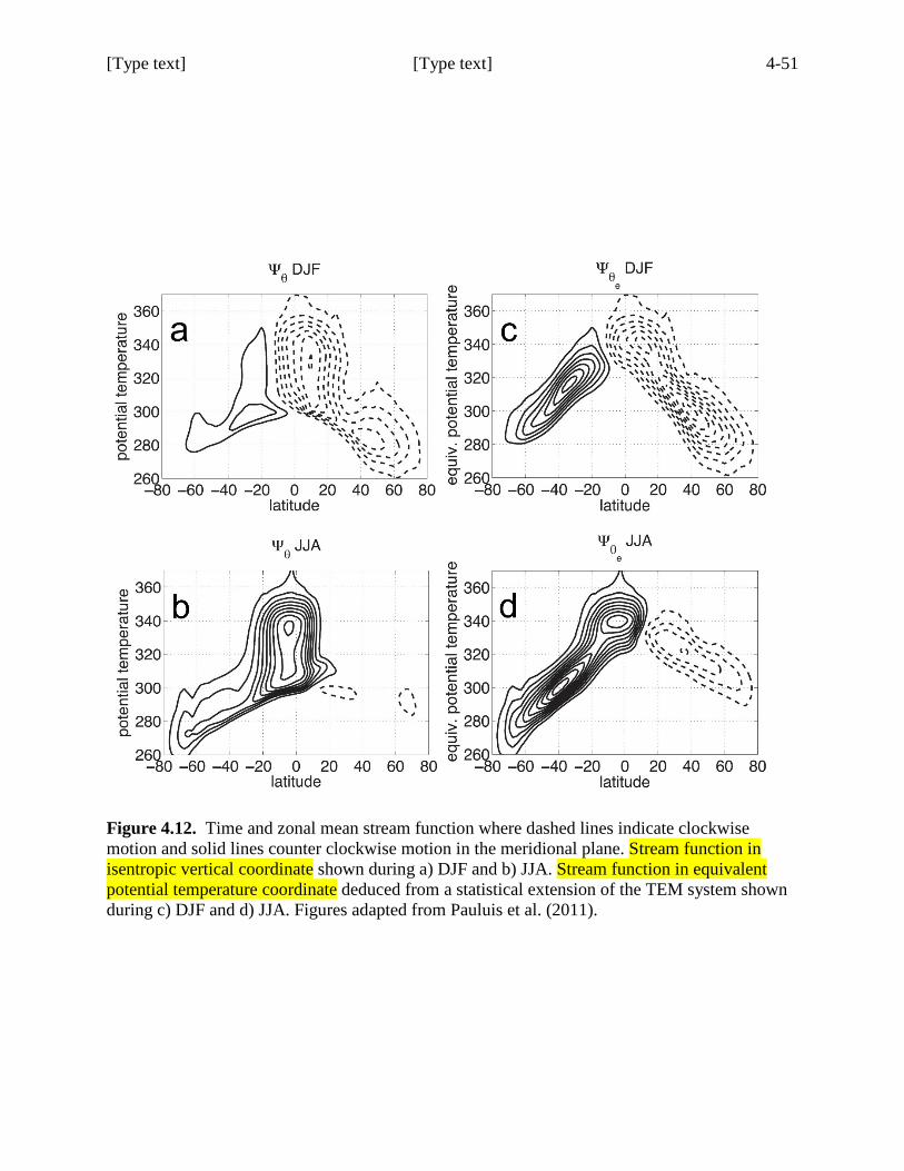
[Type text] [Type text] 4-51

Figure 4.12. Time and zonal mean stream function where dashed lines indicate clockwise motion and solid lines counter clockwise motion in the meridional plane. Stream function in isentropic vertical coordinate shown during a) DJF and b) JJA. Stream function in equivalent potential temperature coordinate deduced from a statistical extension of the TEM system shown during c) DJF and d) JJA. Figures adapted from Pauluis et al. (2011).

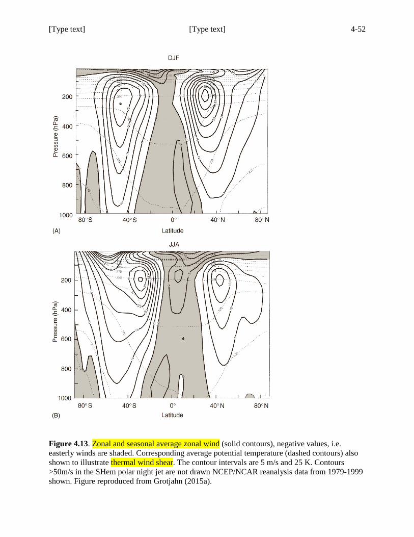
[Type text] [Type text] 4-52

Figure 4.13. Zonal and seasonal average zonal wind (solid contours), negative values, i.e. easterly winds are shaded. Corresponding average potential temperature (dashed contours) also shown to illustrate thermal wind shear. The contour intervals are 5 m/s and 25 K. Contours >50m/s in the SHem polar night jet are not drawn NCEP/NCAR reanalysis data from 1979-1999 shown. Figure reproduced from Grotjahn (2015a).

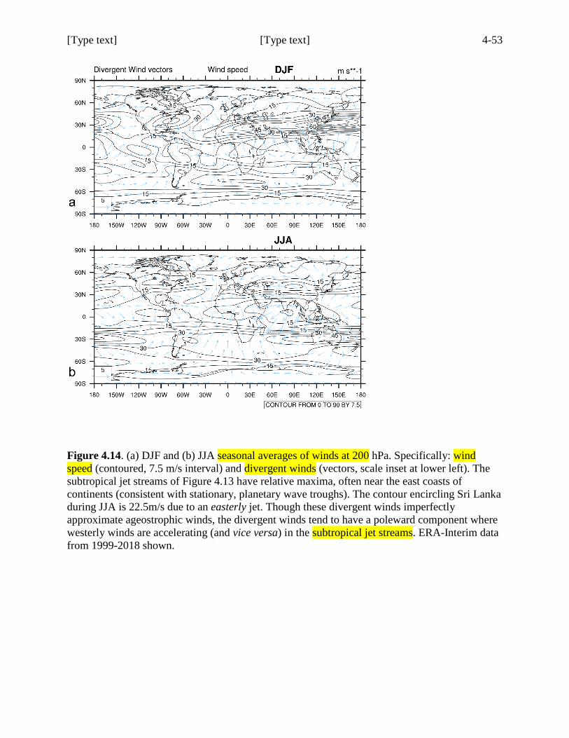
[Type text] [Type text] 4-53

Figure 4.14. (a) DJF and (b) JJA seasonal averages of winds at 200 hPa. Specifically: wind speed (contoured, 7.5 m/s interval) and divergent winds (vectors, scale inset at lower left). The subtropical jet streams of Figure 4.13 have relative maxima, often near the east coasts of continents (consistent with stationary, planetary wave troughs). The contour encircling Sri Lanka during JJA is 22.5m/s due to an easterly jet. Though these divergent winds imperfectly approximate ageostrophic winds, the divergent winds tend to have a poleward component where westerly winds are accelerating (and vice versa) in the subtropical jet streams. ERA-Interim data from 1999-2018 shown.

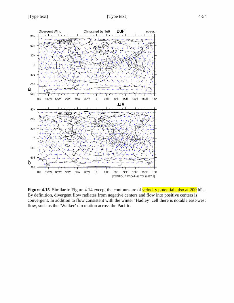
[Type text] [Type text] 4-54

Figure 4.15. Similar to Figure 4.14 except the contours are of velocity potential, also at 200 hPa. By definition, divergent flow radiates from negative centers and flow into positive centers is convergent. In addition to flow consistent with the winter ‘Hadley’ cell there is notable east-west flow, such as the ‘Walker’ circulation across the Pacific.

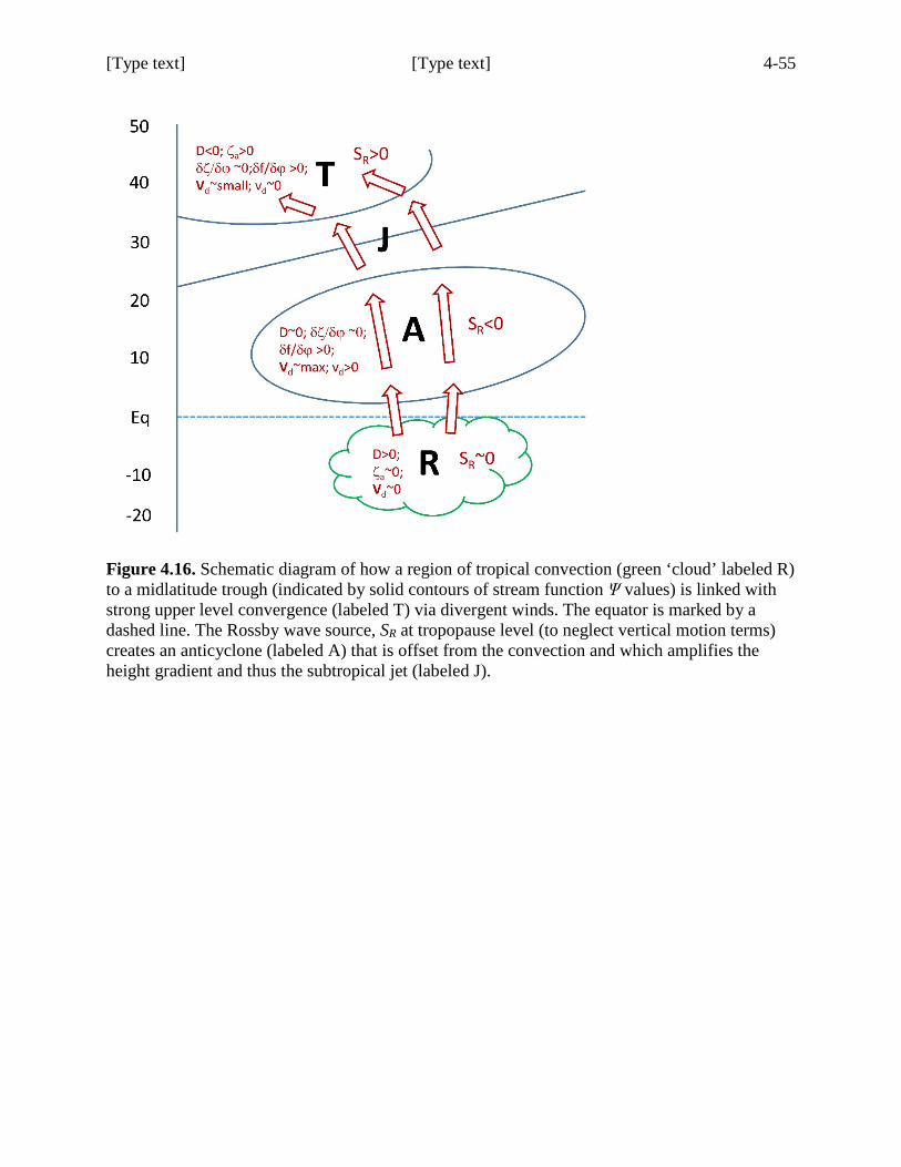
[Type text] [Type text] 4-55

Figure 4.16. Schematic diagram of how a region of tropical convection (green ‘cloud’ labeled R) to a midlatitude trough (indicated by solid contours of stream function Ψ values) is linked with strong upper level convergence (labeled T) via divergent winds. The equator is marked by a dashed line. The Rossby wave source, SR at tropopause level (to neglect vertical motion terms) creates an anticyclone (labeled A) that is offset from the convection and which amplifies the height gradient and thus the subtropical jet (labeled J).

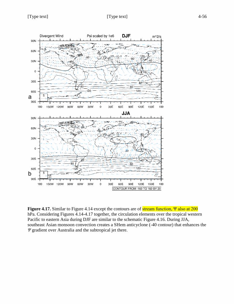
[Type text] [Type text] 4-56

Figure 4.17. Similar to Figure 4.14 except the contours are of stream function, Ψ also at 200 hPa. Considering Figures 4.14-4.17 together, the circulation elements over the tropical western Pacific to eastern Asia during DJF are similar to the schematic Figure 4.16. During JJA, southeast Asian monsoon convection creates a SHem anticyclone (-40 contour) that enhances the Ψ gradient over Australia and the subtropical jet there.

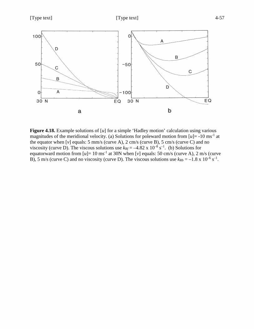
[Type text] [Type text] 4-57

Figure 4.18. Example solutions of [u] for a simple ‘Hadley motion’ calculation using various magnitudes of the meridional velocity. (a) Solutions for poleward motion from [u]= -10 ms-1 at the equator when [v] equals: 5 mm/s (curve A), 2 cm/s (curve B), 5 cm/s (curve C) and no viscosity (curve D). The viscous solutions use kRf = –4.82 x 10–8 s–1. (b) Solutions for equatorward motion from [u]= 10 ms-1 at 30N when [v] equals: 50 cm/s (curve A), 2 m/s (curve B), 5 m/s (curve C) and no viscosity (curve D). The viscous solutions use kRb = –1.8 x 10–6 s–1.

[Type text] [Type text] 4-58 New References Johnson, D.R. 1989: The forcing and maintenance of global monsoonal circulations: an isentropic analysis. Adv. In Geophysics, 31, 43-329. Chapter references: Richard Grotjahn* and Muhtarjan Osman 2006 Remote weather associated with North Pacific subtropical sea-level high properties. Int. J. Climatol. 27: 587–602 (2007) DOI: 10.1002/joc.1423 van Loon (1966) On the annual temperature range over the Southern Oceans. Geographical Review 56: 497–515. Whitaker and Horn (1984) Northern Hemisphere extratropical cyclone activity for four mid-season months. Journal of Climatology 4: 297–310. Simmonds and Murray (1999) Southern extratropical cyclone behavior in ECMWF analyses during the FROST special observing periods. Weather and Forecasting 14: 878–891. Hoskins and Hodges (2002) New perspectives on the Northern Hemisphere winter storm tracks. Journal of the Atmospheric Sciences 59: 1041–1061. Hoskins and Hodges (2005) A new perspective on Southern Hemisphere storm tracks. Journal of Climate 18: 4108–4129. MDS Mesquita NG Kvamstø, A Sorteberg & D E. Atkinson (2008) Climatological properties of summertime extra-tropical storm tracks in the Northern Hemisphere. Tellus 60A: 557–569. DOI: 10.1111/j.1600-0870.2007.00305.x