Chapter 4 Macromechanical Analysis of a Laminate Laminate Analysis Steps

Dr. Autar Kaw

Department of Mechanical Engineering University of South Florida, Tampa, FL 33620

Courtesy of the Textbook

Mechanics of Composite Materials by Kaw

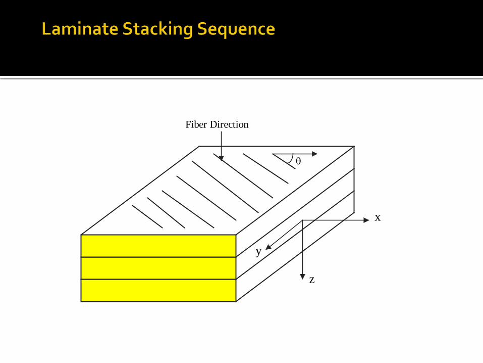
Fiber Direction

θ

x

z

y

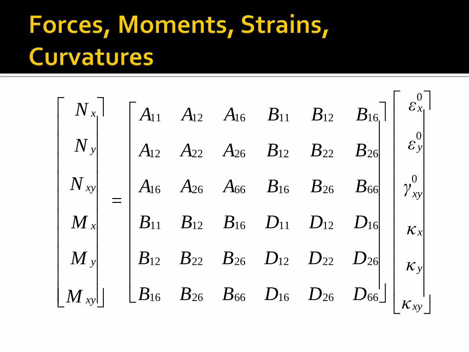
κ

κ

κ

γ

ε

ε

DDDBBB

DDDBBB

DDDBBB

BBBAAA

BBBAAA

BBBAAA

=

M

M

M

N

N

N

xy

y

x

xy

y

x

xy

y

x

xy

y

x

0

0

0

662616662616

262212262212

161211161211

662616662616

262212262212

161211161211

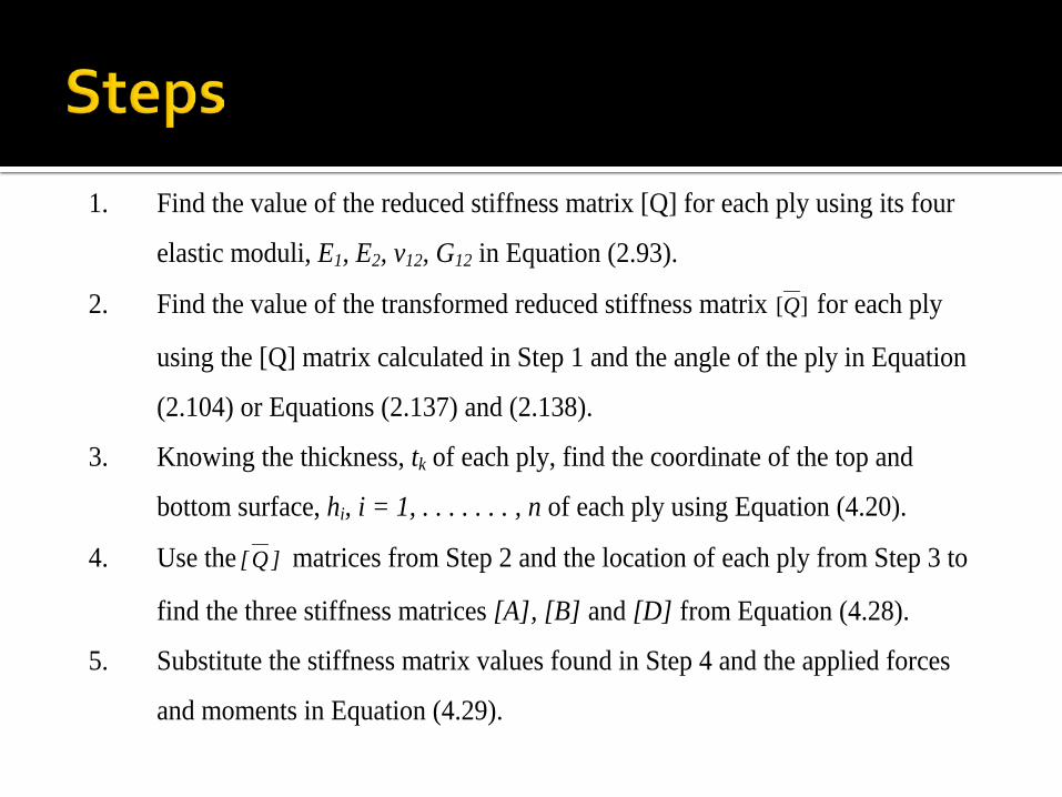
1. Find the value of the reduced stiffness matrix [Q] for each ply using its four

elastic moduli, E1, E2, v12, G12 in Equation (2.93).

2. Find the value of the transformed reduced stiffness matrix ][Q for each ply

using the [Q] matrix calculated in Step 1 and the angle of the ply in Equation

(2.104) or Equations (2.137) and (2.138).

3. Knowing the thickness, tk of each ply, find the coordinate of the top and

bottom surface, hi, i = 1, . . . . . . . , n of each ply using Equation (4.20).

4. Use the ]Q[ matrices from Step 2 and the location of each ply from Step 3 to

find the three stiffness matrices [A], [B] and [D] from Equation (4.28).

5. Substitute the stiffness matrix values found in Step 4 and the applied forces

and moments in Equation (4.29).

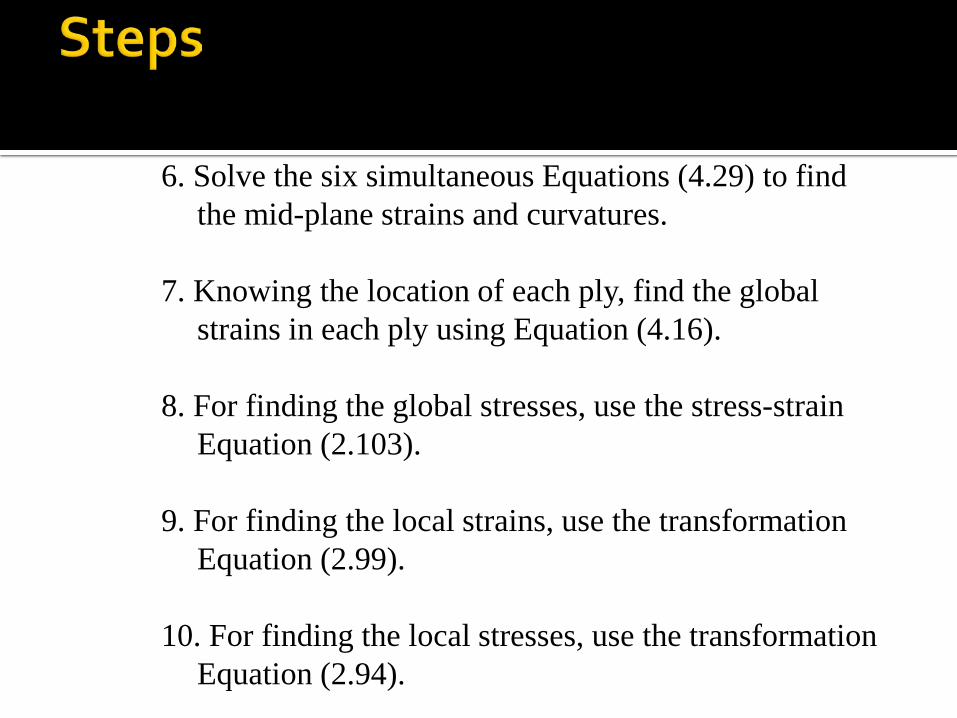
6. Solve the six simultaneous Equations (4.29) to find the mid-plane strains and curvatures.

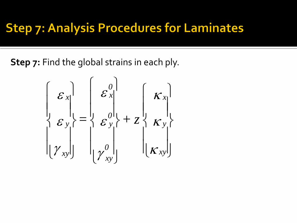
7. Knowing the location of each ply, find the global

strains in each ply using Equation (4.16). 8. For finding the global stresses, use the stress-strain

Equation (2.103). 9. For finding the local strains, use the transformation

Equation (2.99). 10. For finding the local stresses, use the transformation

Equation (2.94).

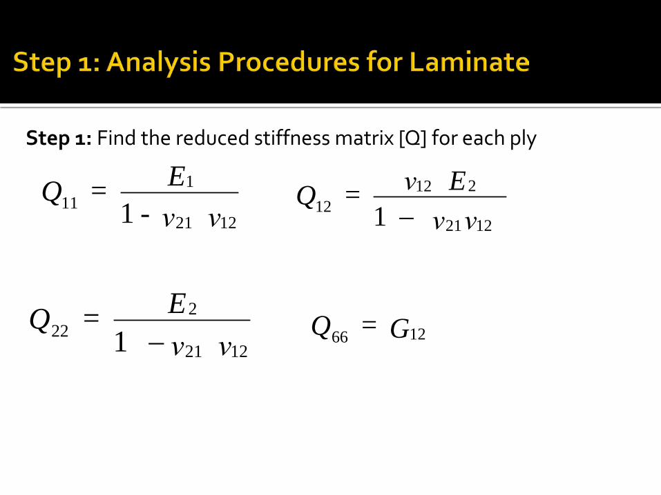
Step 1: Find the reduced stiffness matrix [Q] for each ply

ν ν - E = Q

1221

111 1 νν

E ν = Q1221

21212 1 −

ν ν E = Q

1221

222 1 − G = Q 1266

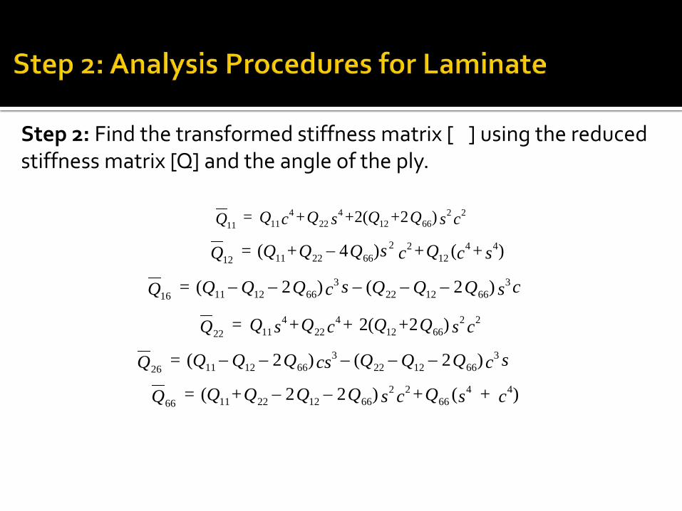
Step 2: Find the transformed stiffness matrix [

] using the reduced stiffness matrix [Q] and the angle of the ply.

csQ+Q+sQ+cQ = Q 226612

422

41111 )2(2

)()4( 4412

2266221112 s+cQ+csQQ+Q = Q −

csQQQscQQQ = Q 3661222

366121116 )2()2( −−−−−

csQ+Q+ cQ+sQ = Q 226612

422

41122 )2(2

scQQQcsQQQ = Q 3661222

366121126 )2()2( −−−−−

)()22( 4466

226612221166 c + sQ+csQQQ+Q = Q −−

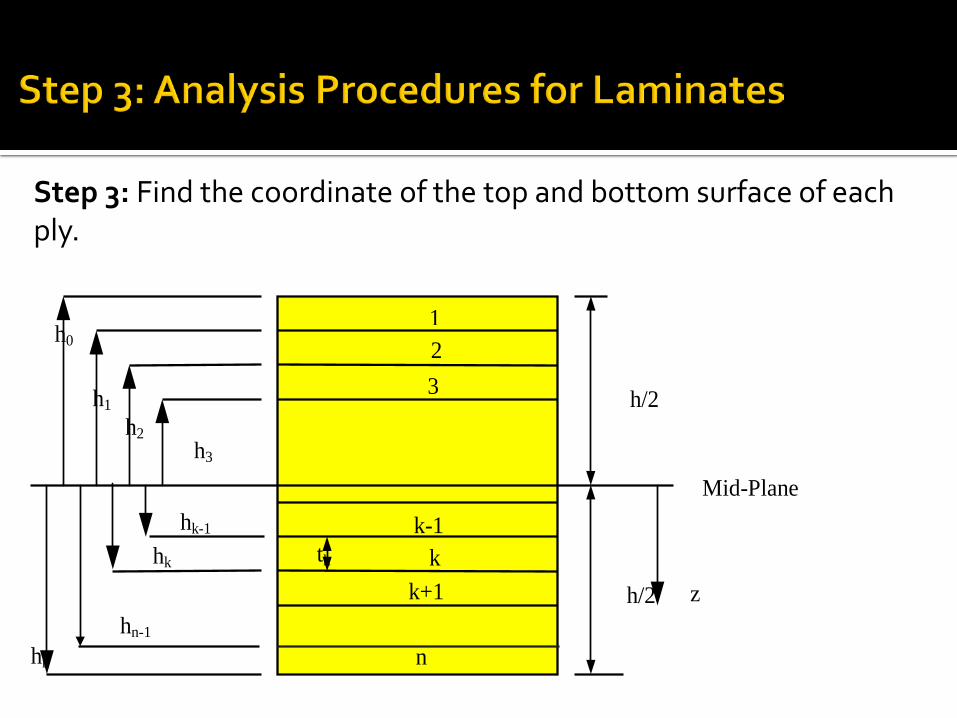
Step 3: Find the coordinate of the top and bottom surface of each ply.

hk-1 hk

hn

h2 h1

h0

Mid-Plane

1 2 3

n

k-1 k

k+1

h3

z

h/2

tk

hn-1 h/2

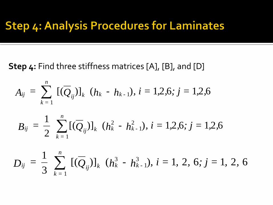
Step 4: Find three stiffness matrices [A], [B], and [D]

621621)()][( 11

,,; j = ,,, i = h - h Q = A k - kkij

n

k = ij ∑

621621)()][(21 2

12

1

,,; j = ,,, i = h - h Q = B k - kkij

n

k = ij ∑

621621),()][(31 3

13

1

, , ; j = , , i = h - h Q = D k - kkij

n

k = ij ∑

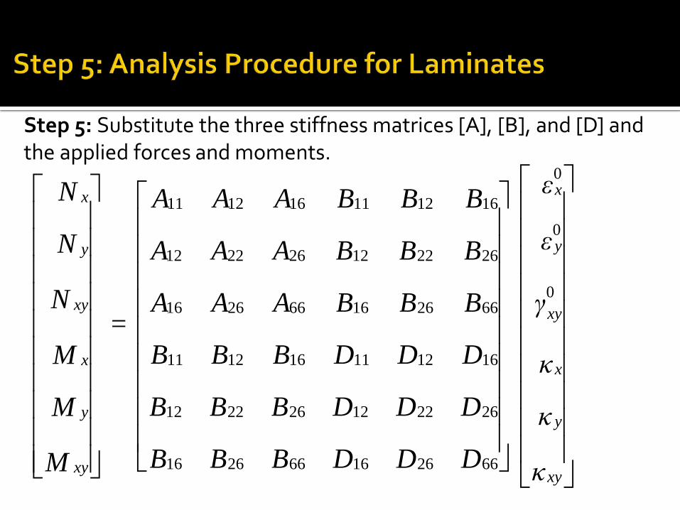
Step 5: Substitute the three stiffness matrices [A], [B], and [D] and the applied forces and moments.

κ

κ

κ

γ

ε

ε

DDDBBB

DDDBBB

DDDBBB

BBBAAA

BBBAAA

BBBAAA

=

M

M

M

N

N

N

xy

y

x

xy

y

x

xy

y

x

xy

y

x

0

0

0

662616662616

262212262212

161211161211

662616662616

262212262212

161211161211

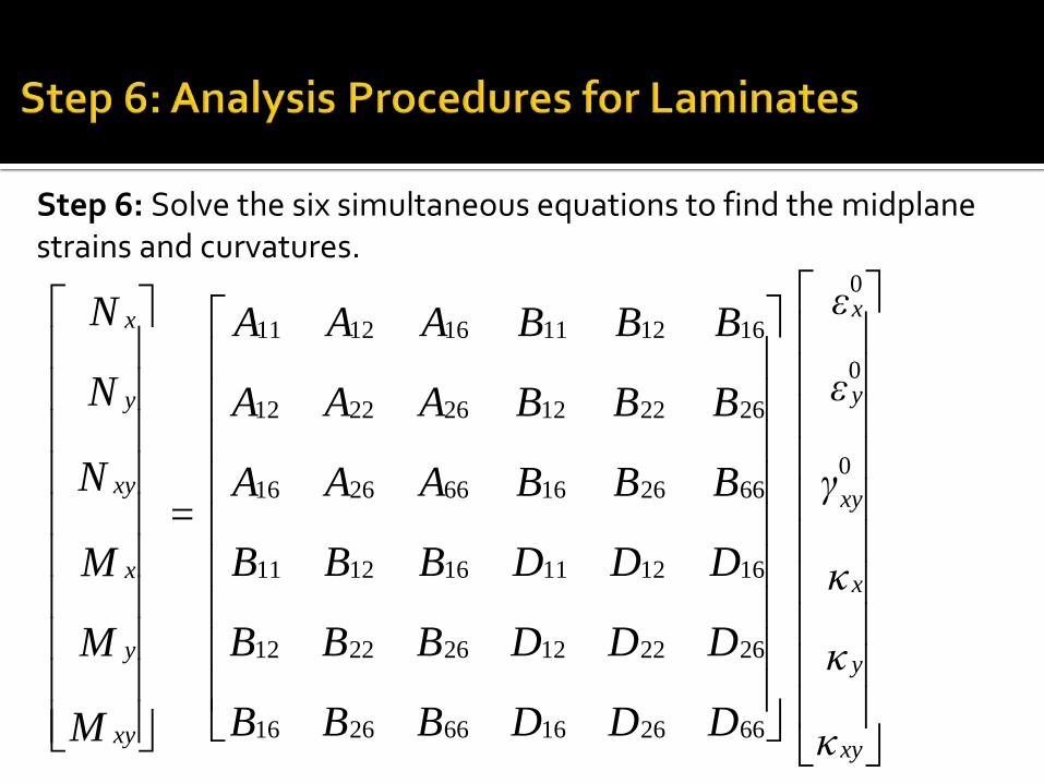
Step 6: Solve the six simultaneous equations to find the midplane strains and curvatures.

κ

κ

κ

γ

ε

ε

DDDBBB

DDDBBB

DDDBBB

BBBAAA

BBBAAA

BBBAAA

=

M

M

M

N

N

N

xy

y

x

xy

y

x

xy

y

x

xy

y

x

0

0

0

662616662616

262212262212

161211161211

662616662616

262212262212

161211161211

Step 7: Find the global strains in each ply.

κ

κ

κ

γ

ε

ε

γ

ε

ε

xy

y

x

0xy

0y

0x

xy

y

x

z + =

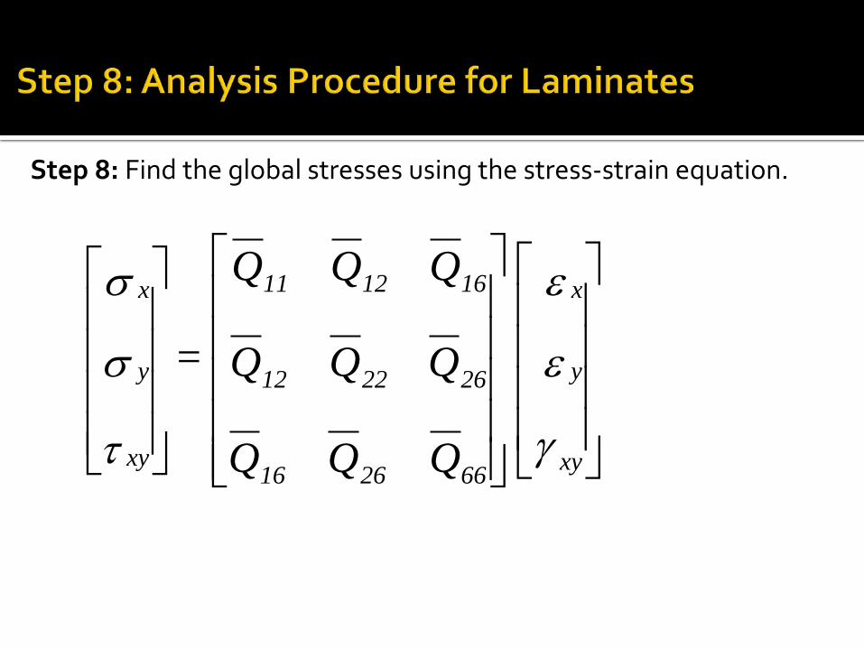
Step 8: Find the global stresses using the stress-strain equation.

γ

ε

ε

τ

σ

σ

xy

y

x

662616

262212

161211

xy

y

x

QQQ

QQQ

QQQ

=

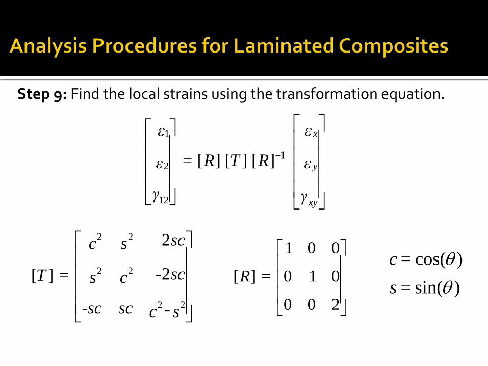
Step 9: Find the local strains using the transformation equation.

−

γ

ε

ε

R T R =

γ

ε

ε

xy

y

x

1

12

2

1

][][][

200

010

001

][ = R

s-csc-sc

sc-cs

scsc

= T22

22

22

2

2

][)cos(θ = c)sin(θ = s

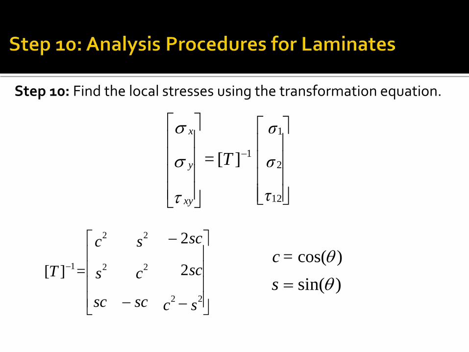
Step 10: Find the local stresses using the transformation equation.

−

τ

σ

σ

T =

xy

y

x

12

2

1

1][

τ

σ

σ

−−

−

−

scscsc

sccs

scsc

=T22

22

22

1 2

2

][)cos(θ= c)sin(θ=s