1

Chapter 4Linear Programming: Modeling Examples

2

Chapter Topics

A Product Mix ExampleA Diet ExampleAn Investment ExampleA Marketing ExampleA Transportation ExampleA Blend Example A Multi-Period Scheduling ExampleA Data Envelopment Analysis Example

2

3

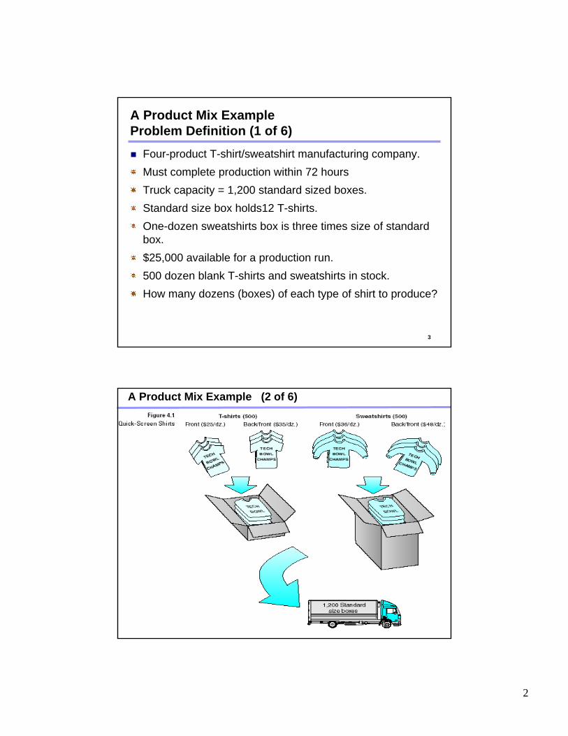
A Product Mix ExampleProblem Definition (1 of 6)

Four-product T-shirt/sweatshirt manufacturing company.Must complete production within 72 hoursTruck capacity = 1,200 standard sized boxes.Standard size box holds12 T-shirts.One-dozen sweatshirts box is three times size of standard box.$25,000 available for a production run.500 dozen blank T-shirts and sweatshirts in stock.How many dozens (boxes) of each type of shirt to produce?

4

A Product Mix Example (2 of 6)

3

5

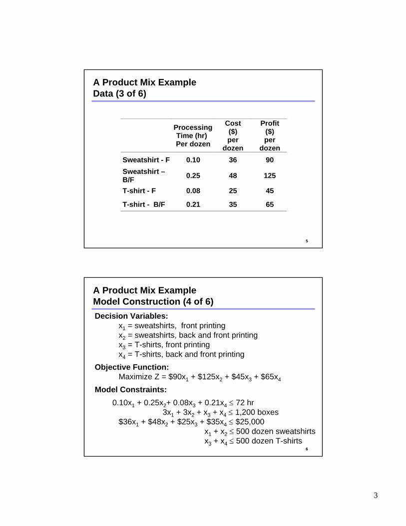
Processing Time (hr) Per dozen

Cost ($) per

dozen

Profit ($) per

dozen Sweatshirt - F 0.10 36 90 Sweatshirt – B/F 0.25 48 125

T-shirt - F 0.08 25 45

T-shirt - B/F 0.21 35 65

A Product Mix ExampleData (3 of 6)

6

Decision Variables:x1 = sweatshirts, front printingx2 = sweatshirts, back and front printingx3 = T-shirts, front printingx4 = T-shirts, back and front printing

Objective Function:Maximize Z = $90x1 + $125x2 + $45x3 + $65x4

Model Constraints:0.10x1 + 0.25x2+ 0.08x3 + 0.21x4 ≤ 72 hr

3x1 + 3x2 + x3 + x4 ≤ 1,200 boxes$36x1 + $48x2 + $25x3 + $35x4 ≤ $25,000

x1 + x2 ≤ 500 dozen sweatshirtsx3 + x4 ≤ 500 dozen T-shirts

A Product Mix ExampleModel Construction (4 of 6)

4

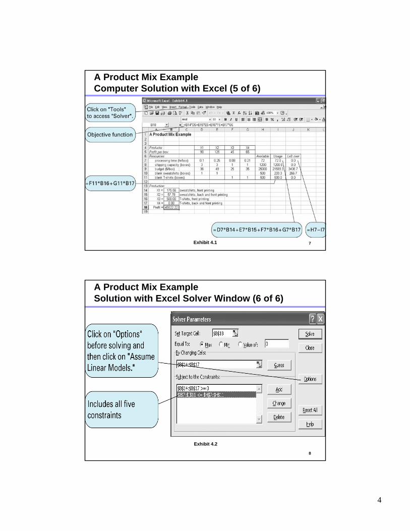
7Exhibit 4.1

A Product Mix ExampleComputer Solution with Excel (5 of 6)

8

Exhibit 4.2

A Product Mix ExampleSolution with Excel Solver Window (6 of 6)

5

9

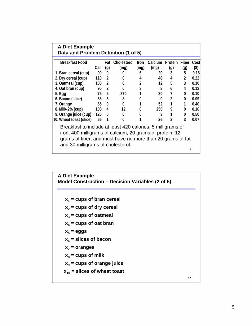
Breakfast to include at least 420 calories, 5 milligrams of iron, 400 milligrams of calcium, 20 grams of protein, 12 grams of fiber, and must have no more than 20 grams of fat and 30 milligrams of cholesterol.

Breakfast Food Cal

Fat(g)

Cholesterol(mg)

Iron (mg)

Calcium(mg)

Protein (g)

Fiber (g)

Cost ($)

1. Bran cereal (cup) 2. Dry cereal (cup) 3. Oatmeal (cup) 4. Oat bran (cup) 5. Egg 6. Bacon (slice) 7. Orange 8. Milk-2% (cup) 9. Orange juice (cup)

10. Wheat toast (slice)

9011010090753565

10012065

0 2 2 2 5 3 0 4 0 1

0 0 0 0

270 8 0 12 0 0

6 4 2 3 1 0 1 0 0 1

204812

830

052

2503

26

3 4 5 6 7 2 1 9 1 3

5 2 3 4 0 0 1 0 0 3

0.18 0.22 0.10 0.12 0.10 0.09 0.40 0.16 0.50 0.07

A Diet ExampleData and Problem Definition (1 of 5)

10

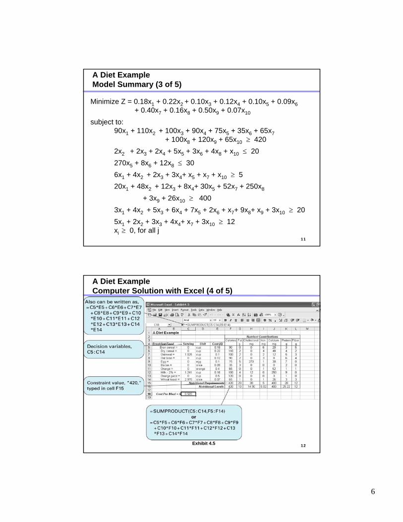
x1 = cups of bran cerealx2 = cups of dry cerealx3 = cups of oatmealx4 = cups of oat branx5 = eggsx6 = slices of baconx7 = orangesx8 = cups of milkx9 = cups of orange juicex10 = slices of wheat toast

A Diet ExampleModel Construction – Decision Variables (2 of 5)

6

11

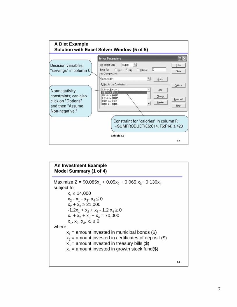
Minimize Z = 0.18x1 + 0.22x2 + 0.10x3 + 0.12x4 + 0.10x5 + 0.09x6 + 0.40x7 + 0.16x8 + 0.50x9 + 0.07x10

subject to:90x1 + 110x2 + 100x3 + 90x4 + 75x5 + 35x6 + 65x7

+ 100x8 + 120x9 + 65x10 ≥ 4202x2 + 2x3 + 2x4 + 5x5 + 3x6 + 4x8 + x10 ≤ 20270x5 + 8x6 + 12x8 ≤ 306x1 + 4x2 + 2x3 + 3x4+ x5 + x7 + x10 ≥ 520x1 + 48x2 + 12x3 + 8x4+ 30x5 + 52x7 + 250x8

+ 3x9 + 26x10 ≥ 4003x1 + 4x2 + 5x3 + 6x4 + 7x5 + 2x6 + x7+ 9x8+ x9 + 3x10 ≥ 205x1 + 2x2 + 3x3 + 4x4+ x7 + 3x10 ≥ 12 xi ≥ 0, for all j

A Diet ExampleModel Summary (3 of 5)

12Exhibit 4.5

A Diet ExampleComputer Solution with Excel (4 of 5)

7

13

Exhibit 4.6

A Diet ExampleSolution with Excel Solver Window (5 of 5)

14

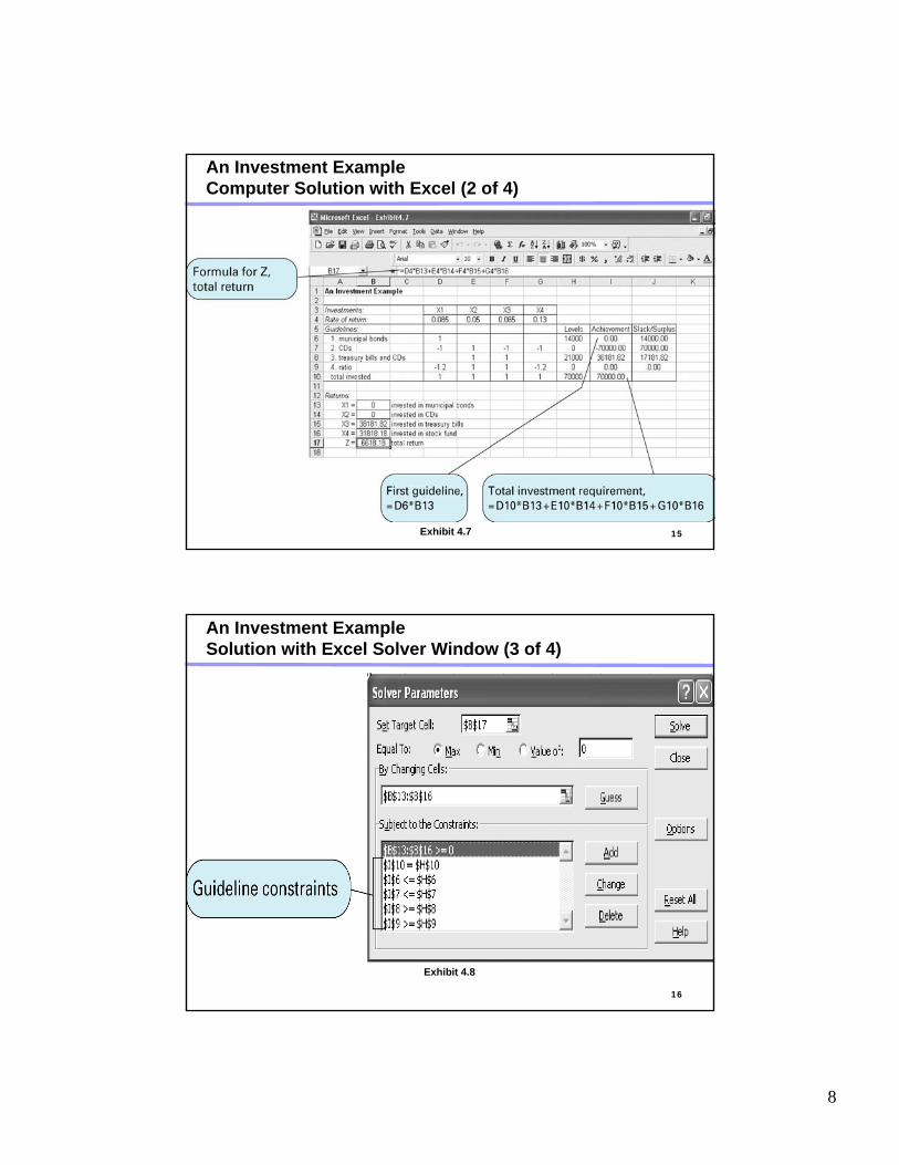
Maximize Z = $0.085x1 + 0.05x2 + 0.065 x3+ 0.130x4subject to:

x1 ≤ 14,000x2 - x1 - x3- x4 ≤ 0x2 + x3 ≥ 21,000-1.2x1 + x2 + x3 - 1.2 x4 ≥ 0x1 + x2 + x3 + x4 = 70,000x1, x2, x3, x4 ≥ 0

wherex1 = amount invested in municipal bonds ($)x2 = amount invested in certificates of deposit ($) x3 = amount invested in treasury bills ($)x4 = amount invested in growth stock fund($)

An Investment ExampleModel Summary (1 of 4)

8

15Exhibit 4.7

An Investment ExampleComputer Solution with Excel (2 of 4)

16

Exhibit 4.8

An Investment ExampleSolution with Excel Solver Window (3 of 4)

9

17Exhibit 4.9

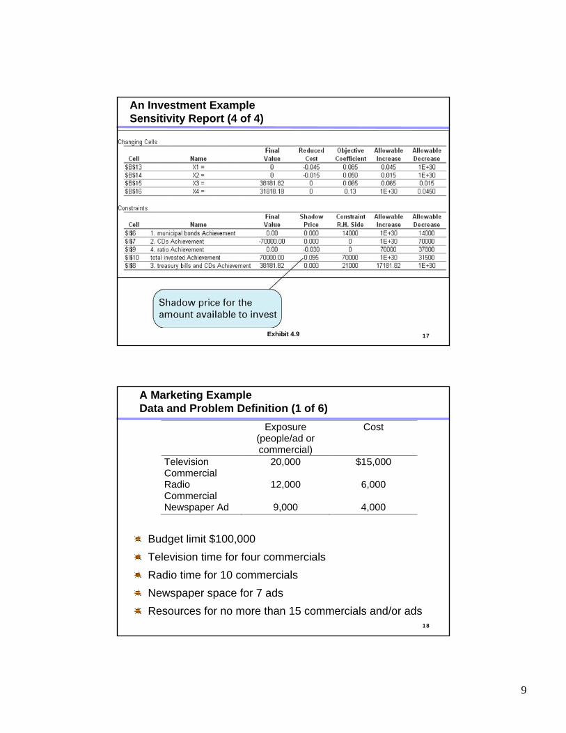
An Investment ExampleSensitivity Report (4 of 4)

18

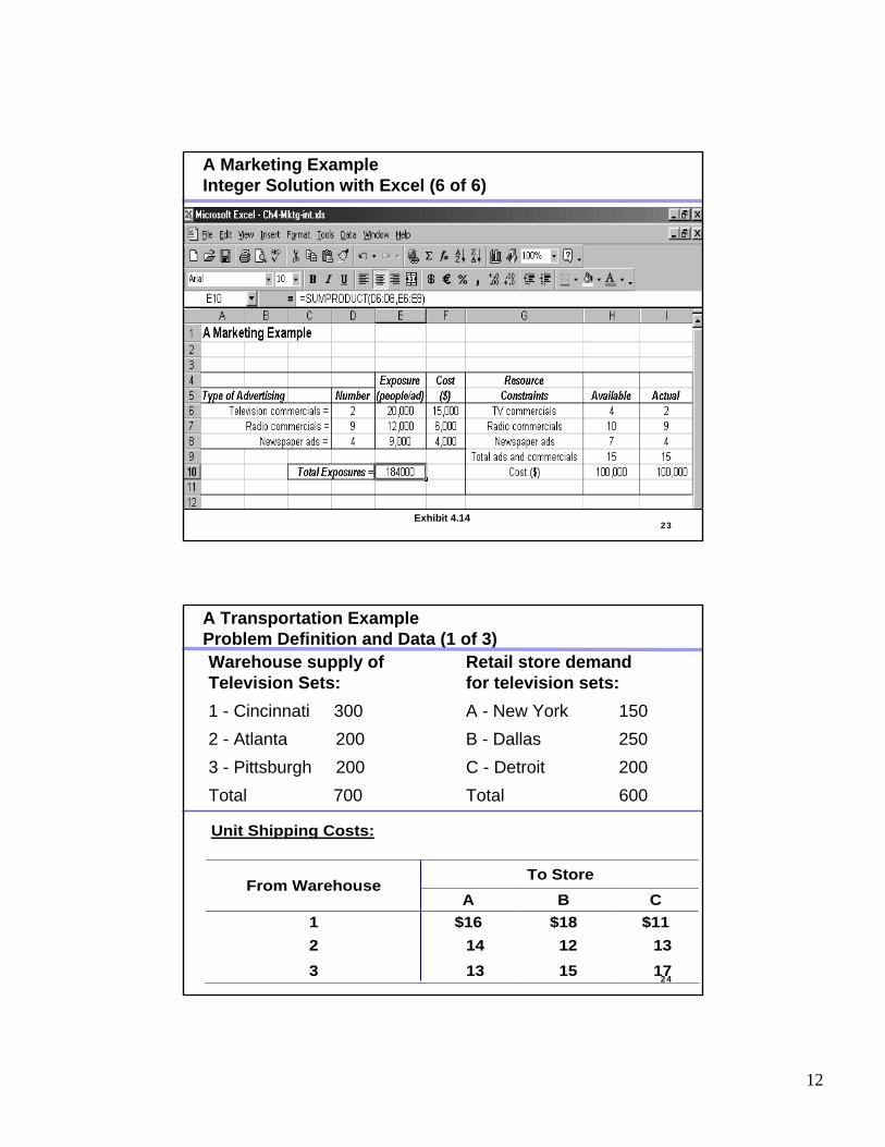
Budget limit $100,000Television time for four commercialsRadio time for 10 commercialsNewspaper space for 7 adsResources for no more than 15 commercials and/or ads

Exposure (people/ad or commercial)

Cost

Television Commercial

20,000 $15,000

Radio Commercial

12,000 6,000

Newspaper Ad 9,000 4,000

A Marketing ExampleData and Problem Definition (1 of 6)

10

19

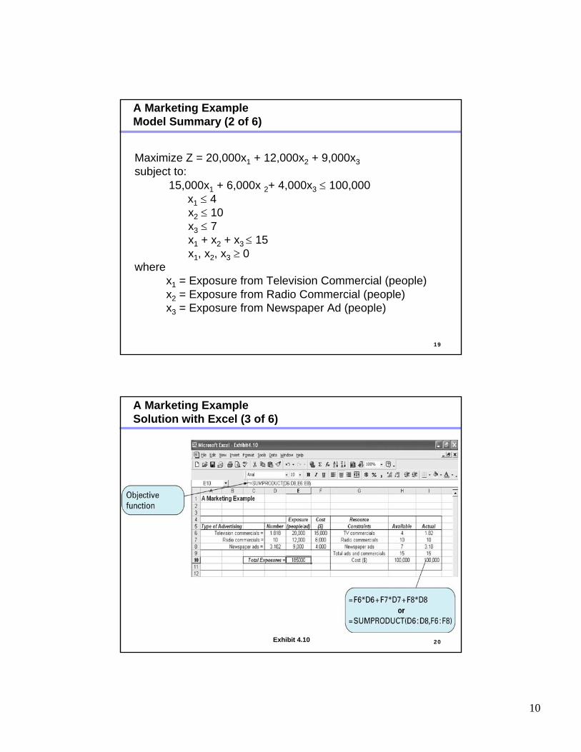
Maximize Z = 20,000x1 + 12,000x2 + 9,000x3subject to:

15,000x1 + 6,000x 2+ 4,000x3 ≤ 100,000x1 ≤ 4x2 ≤ 10x3 ≤ 7x1 + x2 + x3 ≤ 15x1, x2, x3 ≥ 0

wherex1 = Exposure from Television Commercial (people) x2 = Exposure from Radio Commercial (people) x3 = Exposure from Newspaper Ad (people)

A Marketing ExampleModel Summary (2 of 6)

20Exhibit 4.10

A Marketing ExampleSolution with Excel (3 of 6)

11

21

Exhibit 4.11

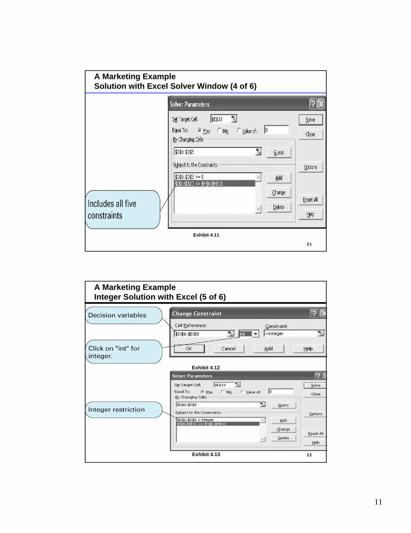
A Marketing ExampleSolution with Excel Solver Window (4 of 6)

22

Exhibit 4.12

Exhibit 4.13

A Marketing ExampleInteger Solution with Excel (5 of 6)

12

23Exhibit 4.14

A Marketing ExampleInteger Solution with Excel (6 of 6)

24

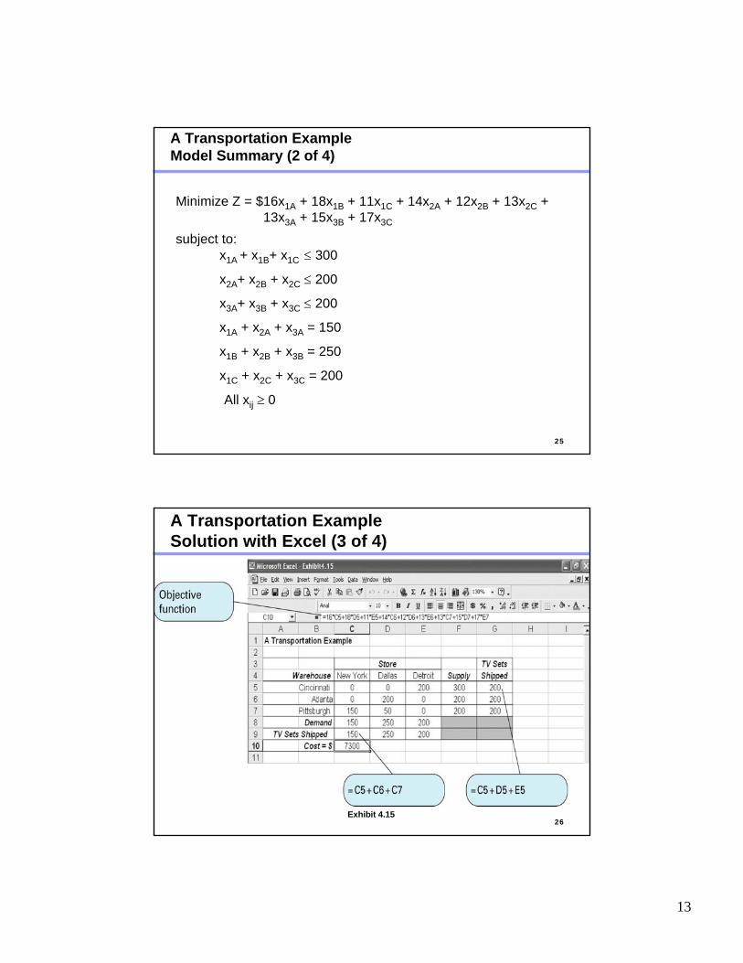
Warehouse supply of Retail store demand Television Sets: for television sets:1 - Cincinnati 300 A - New York 1502 - Atlanta 200 B - Dallas 2503 - Pittsburgh 200 C - Detroit 200 Total 700 Total 600

Unit Shipping Costs:

To Store From Warehouse

A B C 1 $16 $18 $11 2 14 12 13 3 13 15 17

A Transportation ExampleProblem Definition and Data (1 of 3)

13

25

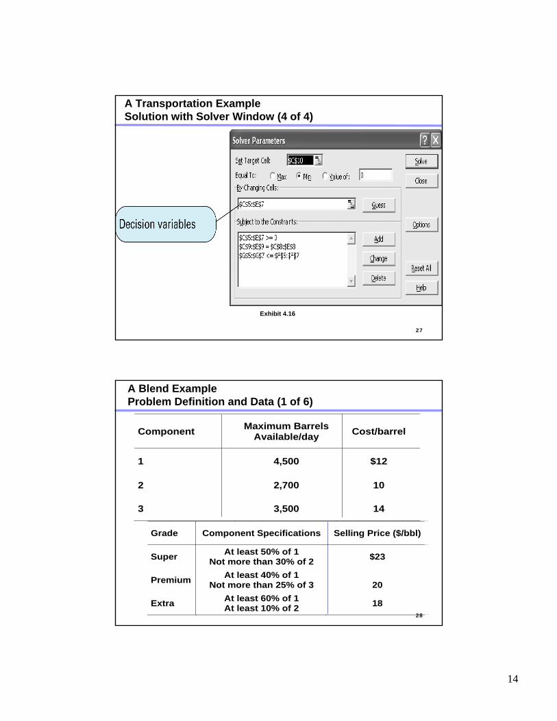
Minimize Z = $16x1A + 18x1B + 11x1C + 14x2A + 12x2B + 13x2C + 13x3A + 15x3B + 17x3C

subject to:x1A + x1B+ x1C ≤ 300

x2A+ x2B + x2C ≤ 200

x3A+ x3B + x3C ≤ 200

x1A + x2A + x3A = 150

x1B + x2B + x3B = 250

x1C + x2C + x3C = 200

All xij ≥ 0

A Transportation ExampleModel Summary (2 of 4)

26Exhibit 4.15

A Transportation ExampleSolution with Excel (3 of 4)

14

27

Exhibit 4.16

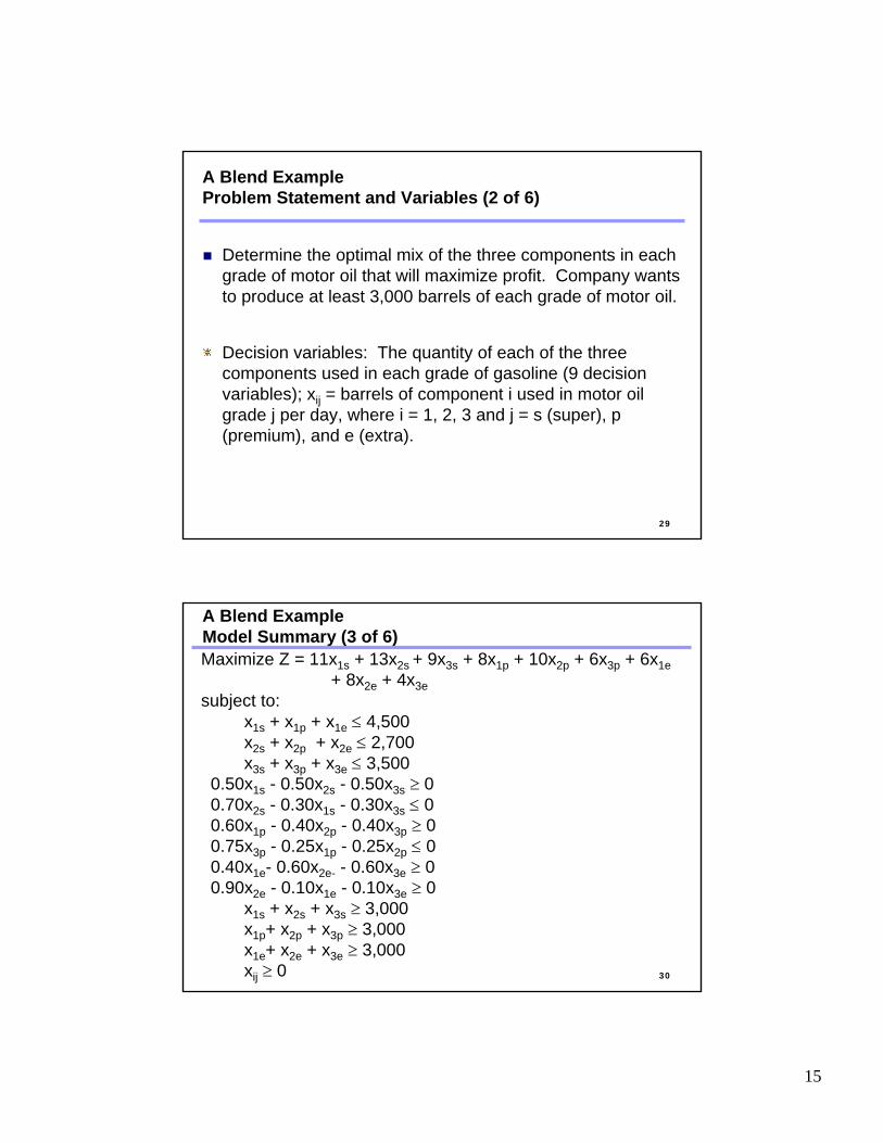
A Transportation ExampleSolution with Solver Window (4 of 4)

28

Component Maximum Barrels Available/day Cost/barrel

1 4,500 $12

2 2,700 10

3 3,500 14

Grade Component Specifications Selling Price ($/bbl)

Super At least 50% of 1 Not more than 30% of 2 $23

Premium At least 40% of 1 Not more than 25% of 3

20

Extra At least 60% of 1 At least 10% of 2 18

A Blend ExampleProblem Definition and Data (1 of 6)

15

29

Determine the optimal mix of the three components in each grade of motor oil that will maximize profit. Company wants to produce at least 3,000 barrels of each grade of motor oil.

Decision variables: The quantity of each of the three components used in each grade of gasoline (9 decision variables); xij = barrels of component i used in motor oil grade j per day, where i = 1, 2, 3 and j = s (super), p (premium), and e (extra).

A Blend ExampleProblem Statement and Variables (2 of 6)

30

Maximize Z = 11x1s + 13x2s + 9x3s + 8x1p + 10x2p + 6x3p + 6x1e+ 8x2e + 4x3e

subject to:x1s + x1p + x1e ≤ 4,500x2s + x2p + x2e ≤ 2,700x3s + x3p + x3e ≤ 3,500

0.50x1s - 0.50x2s - 0.50x3s ≥ 00.70x2s - 0.30x1s - 0.30x3s ≤ 00.60x1p - 0.40x2p - 0.40x3p ≥ 00.75x3p - 0.25x1p - 0.25x2p ≤ 00.40x1e- 0.60x2e- - 0.60x3e ≥ 00.90x2e - 0.10x1e - 0.10x3e ≥ 0

x1s + x2s + x3s ≥ 3,000x1p+ x2p + x3p ≥ 3,000x1e+ x2e + x3e ≥ 3,000xij ≥ 0

A Blend ExampleModel Summary (3 of 6)

16

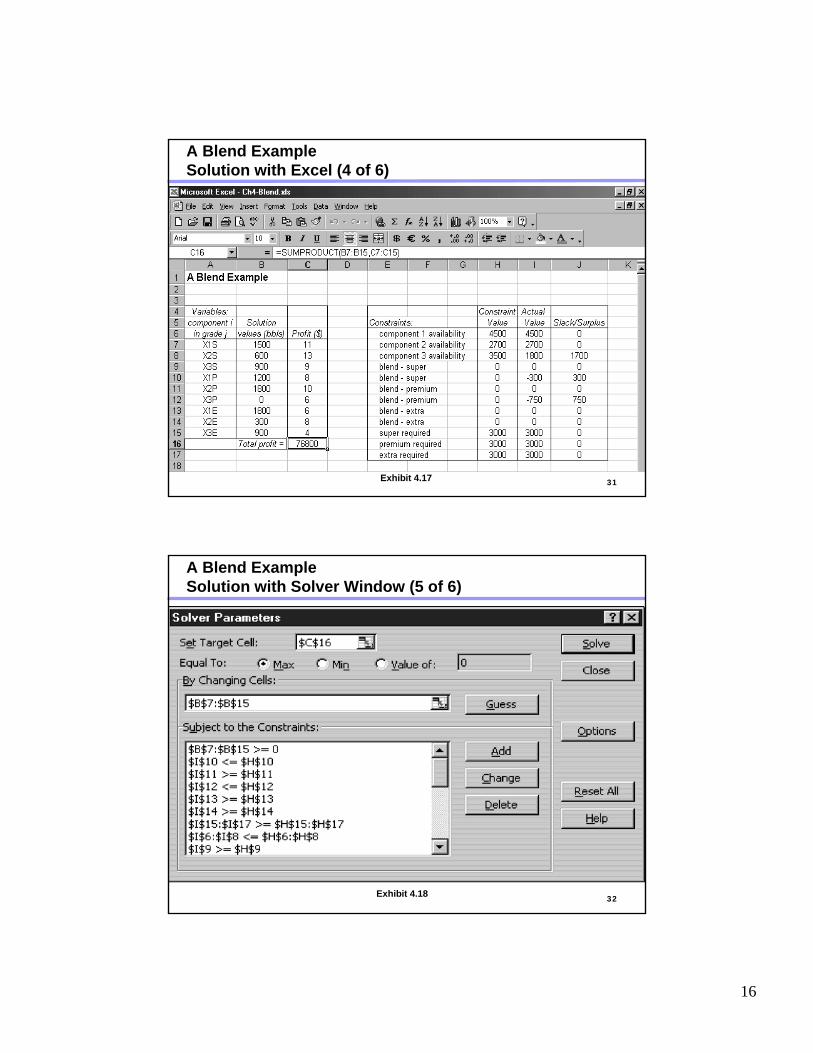
31Exhibit 4.17

A Blend ExampleSolution with Excel (4 of 6)

32Exhibit 4.18

A Blend ExampleSolution with Solver Window (5 of 6)

17

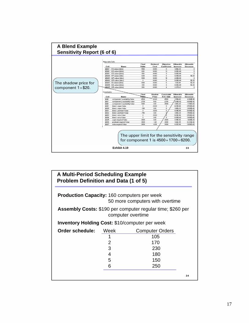
33Exhibit 4.19

A Blend ExampleSensitivity Report (6 of 6)

34

Production Capacity: 160 computers per week50 more computers with overtime

Assembly Costs: $190 per computer regular time; $260 per computer overtime

Inventory Holding Cost: $10/computer per weekOrder schedule: Week Computer Orders

1 1052 1703 2304 1805 1506 250

A Multi-Period Scheduling ExampleProblem Definition and Data (1 of 5)

18

35

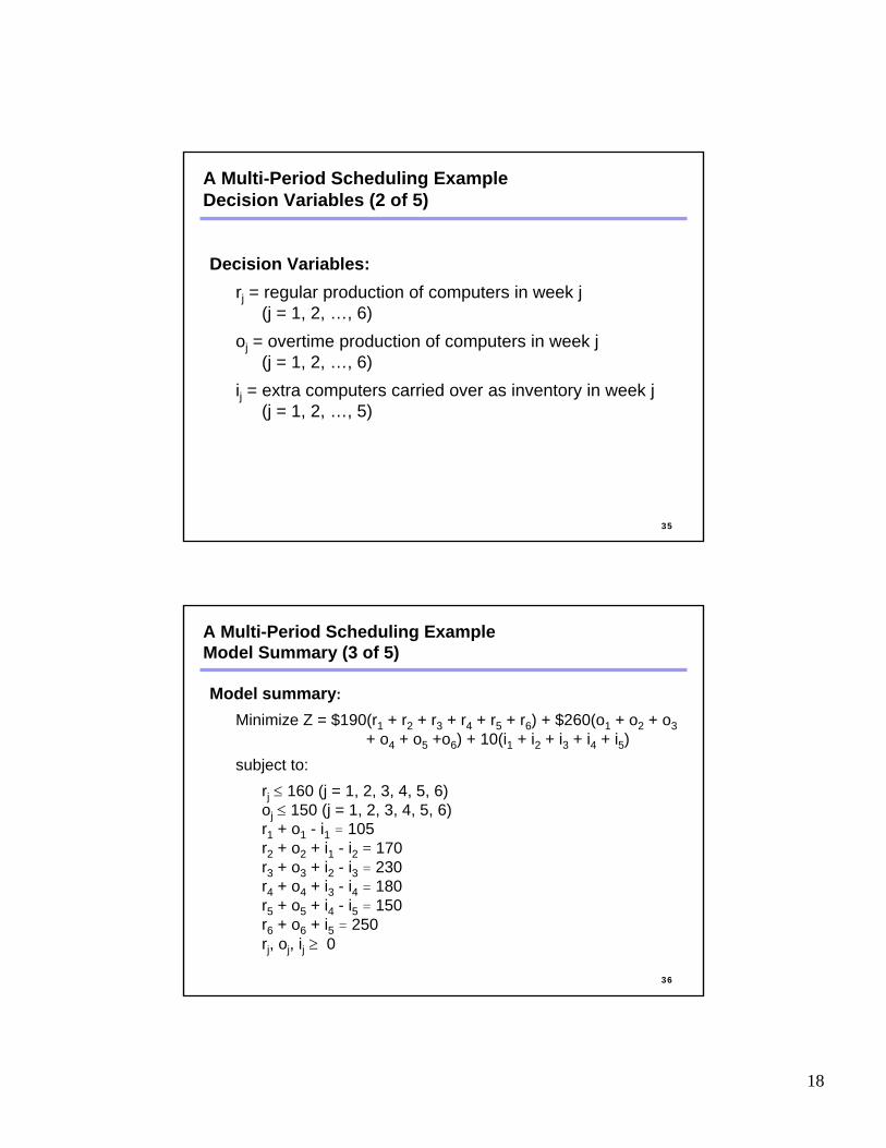
Decision Variables:rj = regular production of computers in week j

(j = 1, 2, …, 6)oj = overtime production of computers in week j

(j = 1, 2, …, 6)ij = extra computers carried over as inventory in week j

(j = 1, 2, …, 5)

A Multi-Period Scheduling ExampleDecision Variables (2 of 5)

36

Model summary:

Minimize Z = $190(r1 + r2 + r3 + r4 + r5 + r6) + $260(o1 + o2 + o3 + o4 + o5 +o6) + 10(i1 + i2 + i3 + i4 + i5)

subject to:rj ≤ 160 (j = 1, 2, 3, 4, 5, 6)oj ≤ 150 (j = 1, 2, 3, 4, 5, 6)r1 + o1 - i1 = 105r2 + o2 + i1 - i2 = 170r3 + o3 + i2 - i3 = 230 r4 + o4 + i3 - i4 = 180r5 + o5 + i4 - i5 = 150r6 + o6 + i5 = 250rj, oj, ij ≥ 0

A Multi-Period Scheduling ExampleModel Summary (3 of 5)

19

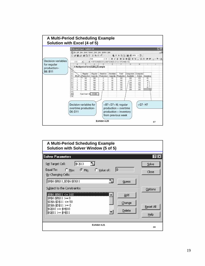
37Exhibit 4.20

A Multi-Period Scheduling ExampleSolution with Excel (4 of 5)

38Exhibit 4.21

A Multi-Period Scheduling ExampleSolution with Solver Window (5 of 5)

20

39

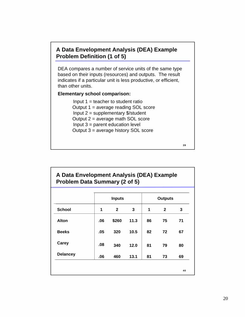
DEA compares a number of service units of the same type based on their inputs (resources) and outputs. The result indicates if a particular unit is less productive, or efficient,than other units.Elementary school comparison:

Input 1 = teacher to student ratioOutput 1 = average reading SOL scoreInput 2 = supplementary $/studentOutput 2 = average math SOL scoreInput 3 = parent education levelOutput 3 = average history SOL score

A Data Envelopment Analysis (DEA) ExampleProblem Definition (1 of 5)

40

Inputs Outputs

School 1 2 3 1 2 3

Alton .06 $260 11.3 86 75 71

Beeks .05 320 10.5 82 72 67

Carey

.08

340

12.0

81

79

80

Delancey .06

460

13.1

81

73

69

A Data Envelopment Analysis (DEA) ExampleProblem Data Summary (2 of 5)

21

41

Decision Variables:xi = a price per unit of each output where i = 1, 2, 3yi = a price per unit of each input where i = 1, 2, 3

Model Summary:Maximize Z = 81x1 + 73x2 + 69x3subject to:

.06 y1 + 460y2 + 13.1y3 = 186x1 + 75x2 + 71x3 ≤.06y1 + 260y2 + 11.3y382x1 + 72x2 + 67x3 ≤ .05y1 + 320y2 + 10.5y381x1 + 79x2 + 80x3 ≤ .08y1 + 340y2 + 12.0y381x1 + 73x2 + 69x3 ≤ .06y1 + 460y2 + 13.1y3

xi, yi ≥ 0

A Data Envelopment Analysis (DEA) ExampleDecision Variables and Model Summary (3 of 5)

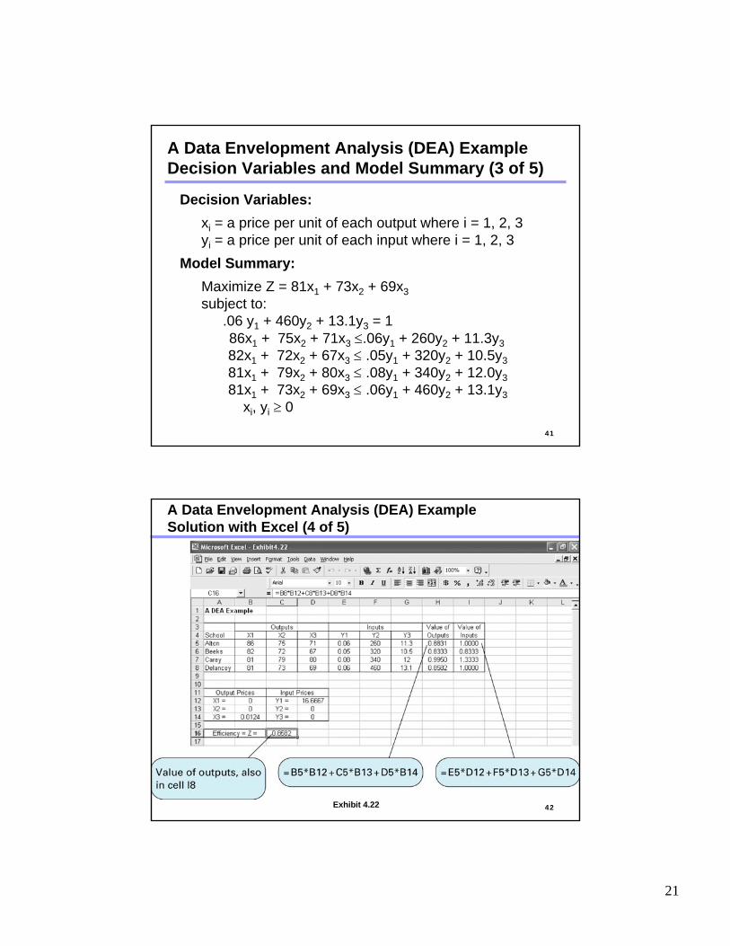
42Exhibit 4.22

A Data Envelopment Analysis (DEA) ExampleSolution with Excel (4 of 5)

22

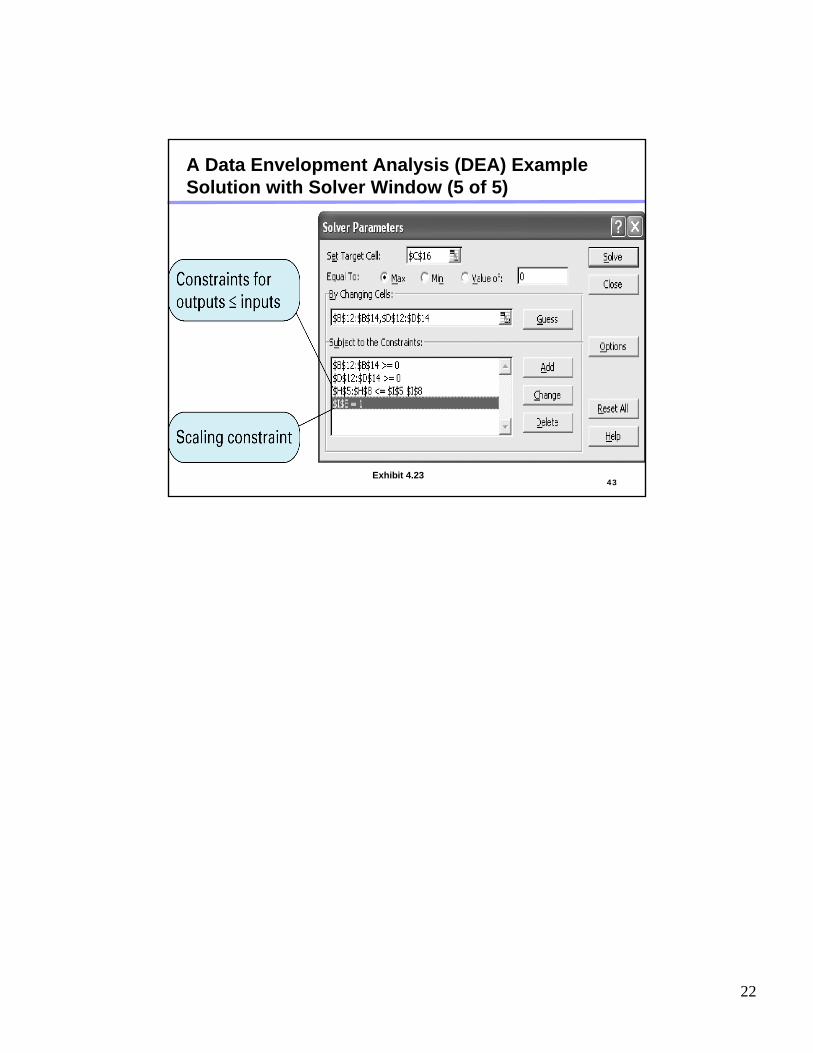
43Exhibit 4.23

A Data Envelopment Analysis (DEA) ExampleSolution with Solver Window (5 of 5)