Embed Size (px)
Citation preview

Page 1
Chapter 4: Linear Programming
Mohammad Farhan Habib Partha Bhaumik
ECS 289I Project Presentation June 5, 2012

Page 2
Outline • Formulations
• Graphical Solutions
• Standard Form
• Computer Solutions
• Sensitivity Analysis
• Applications
• Duality Theory
• Simplex Method
• Interior Point Method

Page 3
Outline • Formulations
• Graphical Solutions
• Standard Form
• Computer Solutions
• Sensitivity Analysis
• Applications
• Duality Theory
• Simplex Method
• Interior Point Method

Page 4
What is an LP?
An LP has • An objective to find the best value for a system • A set of design variables that represents the system • A list of requirements that draws constraints the design variables
The constraints of the system can be expressed as linear equations or inequalities and the objective function is a
linear function of the design variables

Page 5
Types
Linear Program (LP): all variables are real Integer Linear Program (ILP): all variables are integer Mixed Integer Linear Program (MILP): variables are a mix of integer and real number Binary Linear Program (BLP): all variables are binary

Page 6
Formulation
Formulation is the construction of LP models of real problems: • To identify the design/decision variables • Express the constraints of the problem as linear equations or inequalities • Write the objective function to be maximized or minimized as a linear function

Page 7
The Wisdom of Linear Programming
“Model building is not a science; it is primarily an art that is developed mainly
by experience”

Page 8
Example 4.1 Two grades of inspectors for a quality control inspection
• At least 1800 pieces to be inspected per 8-hr day • Grade 1 inspectors:
25 inspections/hour, accuracy = 98%, wage=$4/hour • Grade 2 inspectors:
15 inspections/hour, accuracy= 95%, wage=$3/hour • Penalty=$2/error • Position for 8 “Grade 1” and 10 “Grade 2” inspectors
Let’s get experienced!!

Page 9
Final Formulation for Example 4.1
Page 10
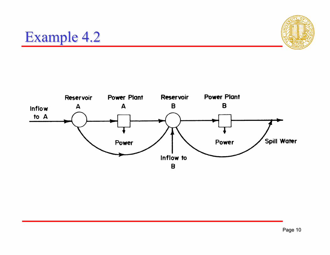
Example 4.2

Page 11
Non-linearity “During each period, up to 50,000 MWh of electricity can be sold at $20.00/MWh, and excess power above 50,000 MWh can only be sold for $14.00/MW”
Piecewise à Linear in the regions (0, 50000) and (50000, ∞)
Page 12
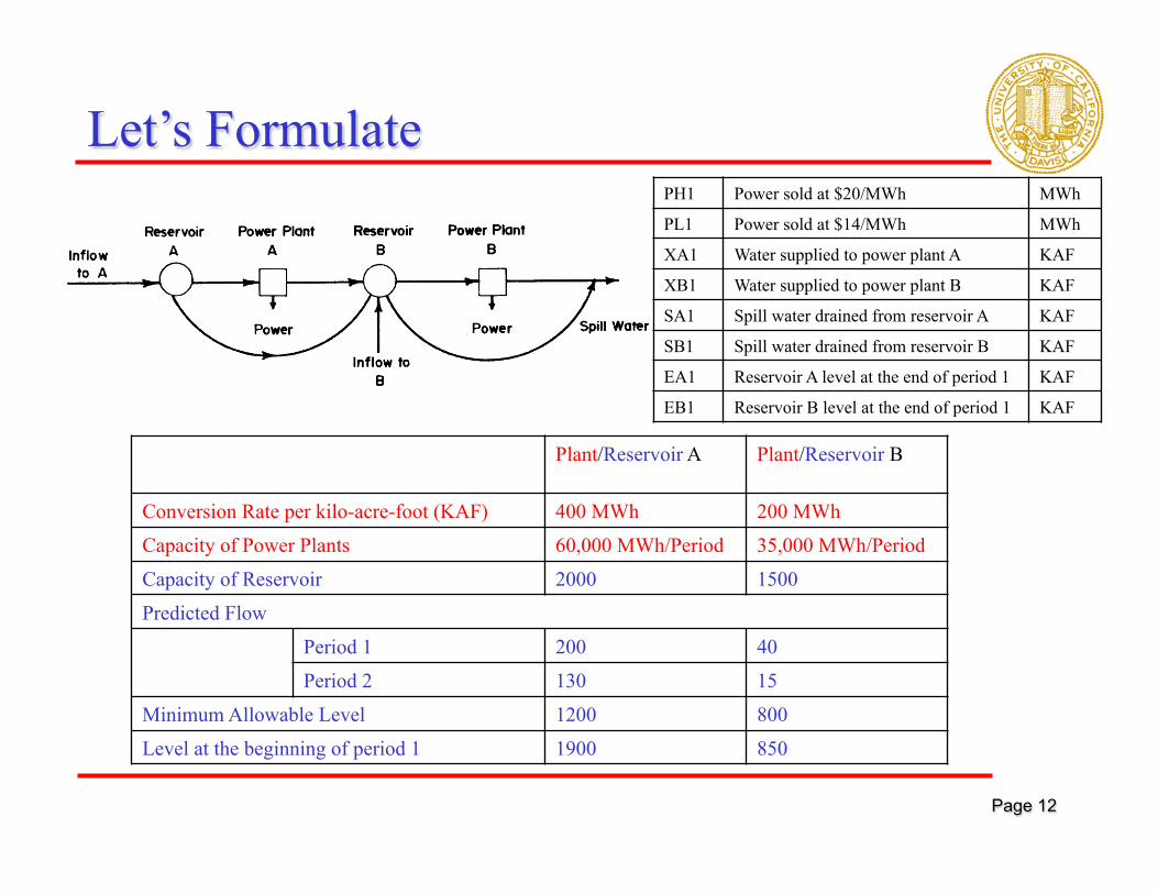
Let’s Formulate
Plant/Reservoir A Plant/Reservoir B Conversion Rate per kilo-acre-foot (KAF) 400 MWh 200 MWh Capacity of Power Plants 60,000 MWh/Period 35,000 MWh/Period Capacity of Reservoir 2000 1500 Predicted Flow
Period 1 200 40 Period 2 130 15
Minimum Allowable Level 1200 800 Level at the beginning of period 1 1900 850
PH1 Power sold at $20/MWh MWh
PL1 Power sold at $14/MWh MWh
XA1 Water supplied to power plant A KAF
XB1 Water supplied to power plant B KAF
SA1 Spill water drained from reservoir A KAF
SB1 Spill water drained from reservoir B KAF
EA1 Reservoir A level at the end of period 1 KAF
EB1 Reservoir B level at the end of period 1 KAF

Page 13
Final Formulation for Example 4.2

Page 14
Outline • Formulations
• Graphical Solutions
• Standard Form
• Computer Solutions
• Sensitivity Analysis
• Applications
• Duality Theory
• Simplex Method
• Interior Point Method

Page 15
Definitions
• Feasible Solution: all possible values of decision variables that satisfy the constraints
• Feasible Region: the set of all feasible solutions
• Optimal Solution: The best feasible solution
• Optimal Value: The value of the objective function corresponding to an optimal solution
Page 16
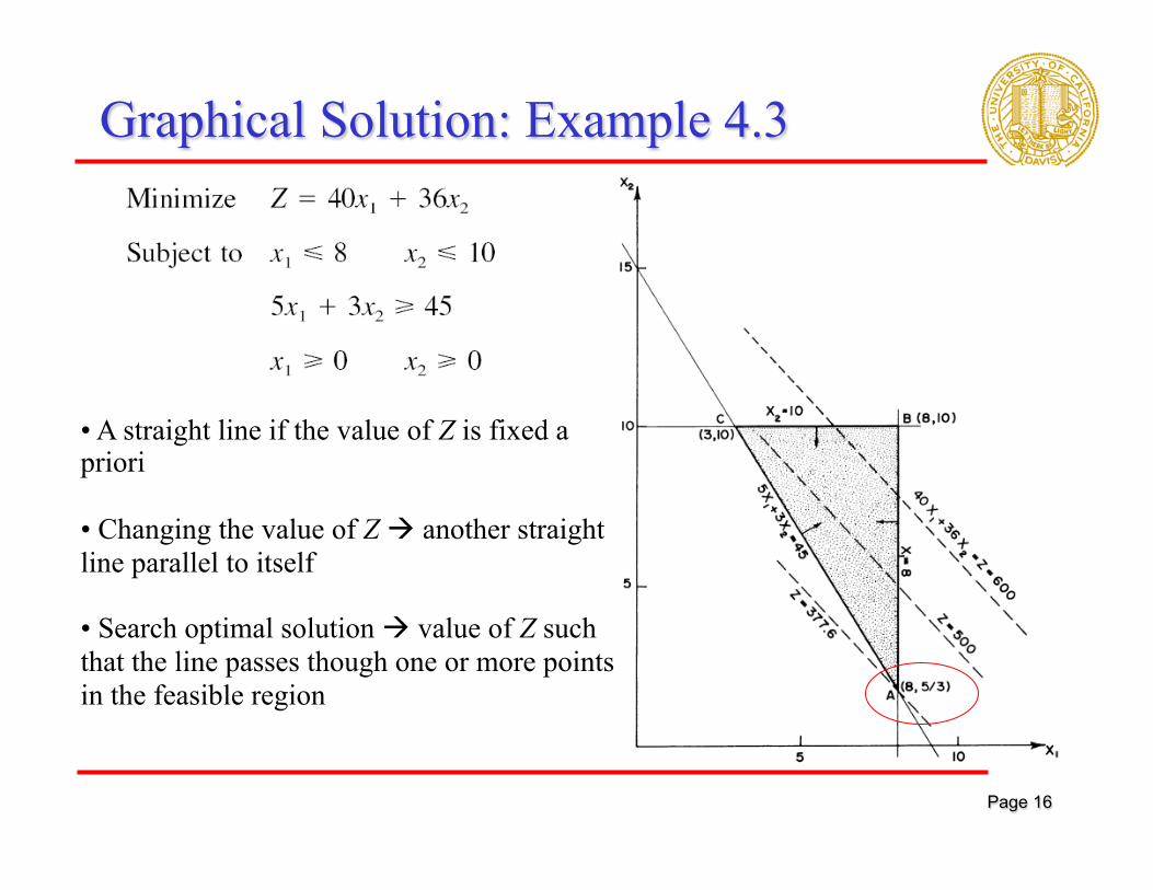
Graphical Solution: Example 4.3
• A straight line if the value of Z is fixed a priori
• Changing the value of Z à another straight line parallel to itself
• Search optimal solution à value of Z such that the line passes though one or more points in the feasible region

Page 17
Graphical Solution: Example 4.4
• All points on line BC are optimal solutions

Page 18
Realizations
• Unique Optimal Solution: only one optimal value (Example 4.1)
• Alternative/Multiple Optimal Solution: more than one feasible solution (Example 4.2)
• Unbounded Optimum: it is possible to find better feasible solutions improving the objective values continuously (e.g., Example 2 without )
Property: If there exists an optimum solution to a linear programming problem, then at least one of the corner points of the feasible region will always qualify to be an optimal solution!

Page 19
Outline • Formulations
• Graphical Solutions
• Standard Form
• Computer Solutions
• Sensitivity Analysis
• Applications
• Duality Theory
• Simplex Method
• Interior Point Method

Page 20
Standard Form (Equation Form)

Page 21
Standard Form (Matrix Form)
(A is the coefficient matrix, x is the decision vector, b is the requirement vector, and c is the profit (cost) vector)

Page 22
Handling Inequalities
Using Bounds
Slack Using Equalities
Surplus

Page 23
Unrestricted Variables
In some situations, it may become necessary to introduce a variable that can assume both positive and negative values!

Page 24
Conversion: Example 4.5

Page 25
Conversion: Example 4.5
Page 26
Recap
Page 27
Outline • Formulations
• Graphical Solutions
• Standard Form
• Computer Solutions
• Sensitivity Analysis
• Applications
• Duality Theory
• Simplex Method
• Interior Point Method

Page 28
Computer Codes • For small/simple LPs:
• Microsoft Excel
• For High-End LP: • OSL from IBM • IBM ILOG CPLEX • OB1 from XMP Software
• Modeling Language: • GAMS (General Algebraic Modeling System) • AMPL (A Mathematical Programming Language)
• Internet • http: / /www.ece.northwestern.edu/otc

Page 29
Outline • Formulations
• Graphical Solutions
• Standard Form
• Computer Solutions
• Sensitivity Analysis
• Applications
• Duality Theory
• Simplex Method
• Interior Point Method

Page 30
Sensitivity Analysis
• Variation in the values of the data coefficients changes the LP problem, which may in turn affect the optimal solution.
• The study of how the optimal solution will change with changes in the input (data) coefficients is known as sensitivity analysis or post-optimality analysis. • Why?
• Some parameters may be controllable à better optimal value • Data coefficients from statistical estimation à identify the one that effects the objective value most à obtain better estimates

Page 31
Example 4.9
100 hr of labor, 600 lb of material, and 300hr of administration per day
Product 1 Product 2 Product 3 Unit profit 10 6 4
Material Needed 10 lb 4 lb 5 lb Admin Hr 2 hr 2 hr 6 hr

Page 32
Solution

Page 33
Outline • Formulations
• Graphical Solutions
• Standard Form
• Computer Solutions
• Sensitivity Analysis
• Applications
• Duality Theory
• Simplex Method
• Interior Point Method

Page 34
Applications of LP
For any optimization problem in linear form with feasible solution time!
Widely used to solve a variety of industrial, social, military and economic optimization problems.

Page 35
Integer Programming
• Integer Linear Program (ILP) • Mixed Integer Linear Program (MILP) • Binary (0-1) Integer Program
• General solution strategy § Solve as an LP, then round off the fractional
values

Page 36
Outline • Formulations
• Graphical Solutions
• Standard Form
• Computer Solutions
• Sensitivity Analysis
• Applications
• Duality Theory
• Simplex Method
• Interior Point Method

Page 37
Duality of LP
Every linear programming problem has an associated linear program called its dual such that a solution to the original linear program also gives a solution to its dual
Solve one, get one free!!

Page 38
Find a Dual
Objective coefficients
Constraint constants
Reversed
Columns into constraints and constraints into columns

Page 39
Duality Theorem
If both the primal and the dual problems are feasible, then they both have optimal solutions such that their values of the
objective functions are equal.

Page 40
Outline • Formulations
• Graphical Solutions
• Standard Form
• Computer Solutions
• Sensitivity Analysis
• Applications
• Duality Theory
• Simplex Method
• Interior Point Method

Page 41
Simplex Method
• LP problem in standard form
Generally m < n
nnxcxcxcZ +++= ... Maximize 2211
11212111 ...a Subject to bxaxax nn =+++
22222121 ...a bxaxax nn =+++
mnmnmm bxaxax =+++ ...a 2211
0,...,1 ≥nxx
.
.
.

Page 42
Canonical (slack) form
• : basic variables • : non-basic variables
• Elementary row operations: § Multiply any equation in the system by a positive or negative number § Add to any equation a constant multiple of any other equation
{ }mxxB ,...,1=
{ }nm xxN ,...,1+=
11111,11 bxaxaxax nnssmm =+++++ ++
rnrnsrsmmrr bxaxaxax =+++++ ++ 11, mnmnsmsmmmm bxaxaxax =+++++ ++ 11,
Gauss-Jordan Elimination Scheme
Page 43
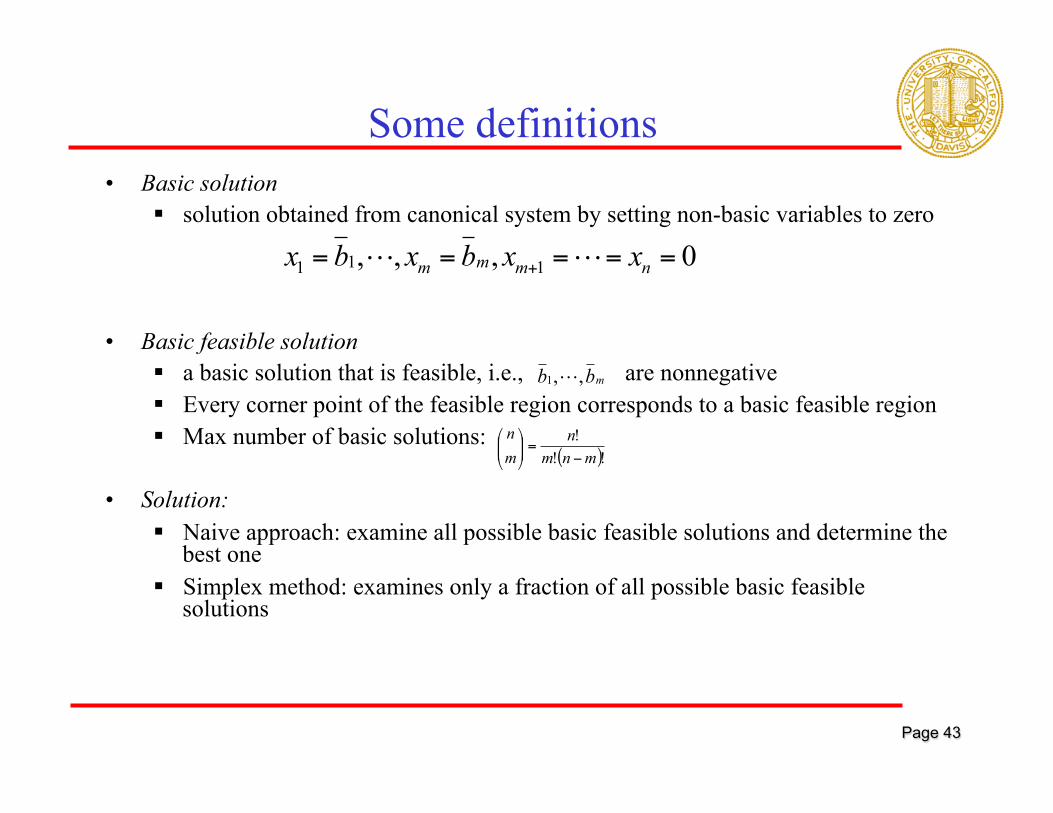
Some definitions • Basic solution
§ solution obtained from canonical system by setting non-basic variables to zero
• Basic feasible solution § a basic solution that is feasible, i.e., are nonnegative § Every corner point of the feasible region corresponds to a basic feasible region § Max number of basic solutions:
• Solution: § Naive approach: examine all possible basic feasible solutions and determine the
best one § Simplex method: examines only a fraction of all possible basic feasible
solutions
0,,, 111 ===== + nmmm xxbxbx
( )!!!mnm
nmn
−=⎟⎟
⎠
⎞⎜⎜⎝
⎛
mbb ,,1

Page 44
Simplex Method
• Adjacent basic feasible solution § differs from the present basic feasible solution in exactly one basic variable
• Optimality criterion § When every adjacent basic feasible solution has objective function value lower
than the present solution
• General Steps 1. Start with an initial basic feasible solution 2. Improve the initial solution if possible by finding an adjacent basic feasible
solution with a better objective function value • It implicitly eliminates those basic feasible solutions whose objective
function values are worse and thereby a more efficient search 3. When a basic feasible solution cannot be improved further, simplex terminates
and return this optimal solution

Page 45
• Assume that we have an initial basic feasible solution as follows:
Nov. 14, 2007
mibx ii ,,1for 0 :Basic =≥=
nmxj ,,1jfor 0 :Nonbasic +==
( )mB xxx ,,1=
( )mB ccc ,,1=
mmBB bcbcxcZ ++== 11
Simplex Method: Step 2

Page 46
Simplex Method: Step 2
• Adjacent feasible solution § The value of nonbasic variable has been increased from 0 to 1 sx
isisi bxax =+
miabx isii ,,1for =−=1=sx
sjnmjx j ≠+== and ,,1for 0
( ) sisi
m
ii cabcZ +−=∑
=1
( ) is
m
iisi
m
iisisi
m
iis accbccabcc ∑∑∑
===
−=−+−=111
Actual profit Relative profit
Inner product rule

Page 47
Simplex Method: Step 2
• Condition of Optimality: • Z will be increase by units for every unit increase of
variablesbasic-non allfor 0≤scsc sx
Should we increase as much as possible?
sx
mixabx sisii ,,1for =−=
⎥⎦
⎤⎢⎣
⎡=
>is
ias a
bxis 0min max ⎥
⎦
⎤⎢⎣
⎡=
rs
r
ab
Minimum-ratio rule
iababxrs
risii allfor ⎟⎟
⎠
⎞⎜⎜⎝
⎛−=
rs
rs abx =
sjnmjx j ≠+== and ,,1for 0

Page 48
Illustrative Example

Page 49
Illustrative Example
is
m
iiss accc ∑
=
−=1
Relative Profit:
Basic Variables: 0543 === ccc
Non-Basic Variables: 2,3 21 == cc
Current solution is not optimal, is chosen as new basic variable 1xWhich variable to replace?
Is the current solution optimal?
⎥⎦
⎤⎢⎣
⎡=
>is
ias a
bxis 0min max Minimum-ratio rule
13 4 xx +=
14 314 xx −=
15 3 xx −=
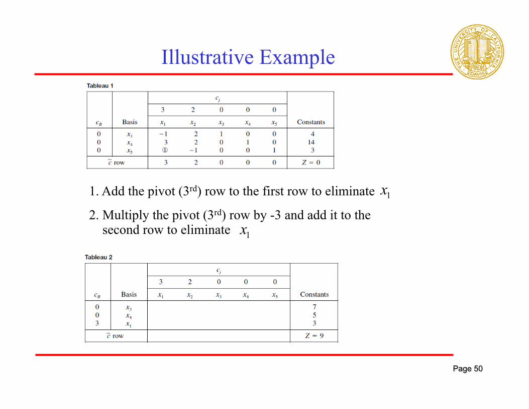
Page 50
Illustrative Example
1. Add the pivot (3rd) row to the first row to eliminate 1x2. Multiply the pivot (3rd) row by -3 and add it to the second row to eliminate 1x

Page 51
Summary of Computational Steps

Page 52
Minimization Problems
• Convert the minimization problem to a maximization problem by multiplying the objective function by -1.
• Modify step 4 § If all the coefficients in the row are positive or
zero, the current basic feasible solution is optimal. Otherwise, select the nonbasic variable with the lowest (most negative) value in the row to enter the basis.
c
c

Page 53
Outline • Formulations
• Graphical Solutions
• Standard Form
• Computer Solutions
• Sensitivity Analysis
• Applications
• Duality Theory
• Simplex Method
• Interior Point Method

Page 54
Interior Point Methods (Karmarkar’s algorithm)
• Interior point method becomes competitive for § very “large” problems, e.g., § some special classes of problems such as multi-period problems
000,10≥+ nm

Page 55
Interior Point Method

Page 56
Computation Steps
• 1. Find an interior point solution to begin the method § Interior points:
• 2. Generate the next interior point with a lower objective function value § Centering: it is advantageous to select an interior point at the
“center” of the feasible region § Steepest Descent Direction
• 3. Test the new point for optimality § where is the objective function of the dual
problem
{ }0xbAxx >= 000 ,|
ε<− wbxc TT wbT

Page 57
Step-2: Generate the Next Interior Point

Page 58
Descent Direction

Page 59
Feasible Direction

Page 60
Illustration of Karmarkar’s Principles

Page 61
How to Center an Interior Point
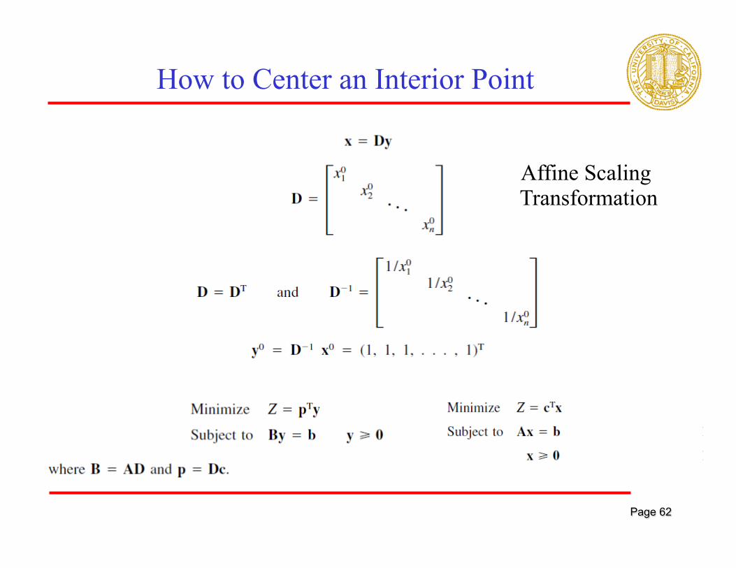
Page 62
How to Center an Interior Point
Affine Scaling Transformation

Page 63
Feasible and Descent Direction
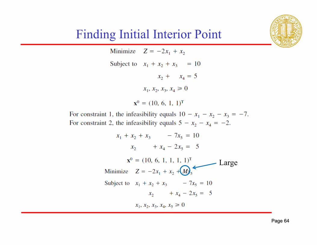
Page 64
Finding Initial Interior Point
Large

Page 65
Conclusion
• LP – linear constraints and linear objective functions
• Easy to solve computationally • Wide range of commercial solvers available • Two major methods – simplex and interior point • Applied to solve various practical real-world
optimization problems – military, economic, industrial, social