Chapter 4: Impact of Future Scenarioslib.icimod.org/record/21652/files/c_attachment_103_1834.pdf · Chapter 4: Impact of Future Scenarios ... availability, flood generation potential,

253Chapter 4 - Impact of the FChapter 4 - Impact of the FChapter 4 - Impact of the FChapter 4 - Impact of the FChapter 4 - Impact of the Future Scenariosuture Scenariosuture Scenariosuture Scenariosuture Scenarios

1 Sorooshian and Gupta (1995)

Chapter 4: Impact of Future Scenarios

“Model results are only as reliable as the model assumptions”(S. Sorooshian and V.K. Gupta)1

This chapter first presents a review of modelling exercises conducted in the HKH region. Forthe prediction of future parameters important to water availability, flood generation, andsediment transport in the catchments — water balance and streamflow in particular — threemodels were applied to the data observed from the Jhikhu Khola catchment. The models arebriefly described and the calibration of all models is discussed. Three scenarios arepresented and their impact on the water balance, water availability, and the streamflowsestimated.

It is important to note that the calculation of scenarios is in its preliminary stages and willreceive further attention in the coming Phase 3 of the project. Therefore the results belowshould be considered initial trials with first successes and failures.

In a time of great consciousness about change, the desire to predict the future is felt increasingly.Unprecedented changes are likely to occur, such as climate change (IPCC 1998), globalisation(Jodha 2000; in print), or the collapse of the natural resource base due to population pressure inmany parts of the world (Allen 2000). The impact of these changes on the hydrological cycle andprocesses cannot be foreseen, due to the limitations of hydrological measurement techniques(Beven 2001). Such an impact can only be simulated and approximated by the use of varioustechniques. At the same time, computer power has increased many times over in recent decadesand can now support complex systems analyses. Complex systems have to be described in order tominimise haphazard assumptions (see citation above).

Over the last century a large amount of data has been collected which can provide a firmunderpinning to these analyses. This is certainly correct for large parts of the developed world. Fordeveloping countries, however, the database for this kind of analyses is limited and furthermarginalised in the mountainous parts of these countries. A number of global water availabilityscenarios have been presented (e.g., Alcamo et al. 2000; Shiklamonov 2000; Seckler et al. 1998) andwere briefly discussed in Chapter 1. On a smaller scale, presentations of the likely impact ofchanges in driving forces, such as climate, population, or policy decisions in this region, have beendetailed in numerous studies. Some of these studies with respect to hydrological modelling arediscussed below.

Note:Note:Note:Note:Note: The modelling was only carried out in the Jhikhu Khola catchment, mainly for reasonsof data availability. The first year will have to be set aside in order to be able to simulate theboundary conditions. For statistical reasons, Sorooshian and Gupta (1995) suggest that twoto three years of calibration data are sufficient. This suggests that at least three completeyears of data and a first monsoon are required, i.e., 1997 (monsoon) to 2000. An additionalone to two years are then required for the validation of the models. With the availability of the2001 and 2002 data the models can also be applied in the other catchments.

254 WWWWWater Balances, Floods and Sediment Tater Balances, Floods and Sediment Tater Balances, Floods and Sediment Tater Balances, Floods and Sediment Tater Balances, Floods and Sediment Transport in the Hindu Kransport in the Hindu Kransport in the Hindu Kransport in the Hindu Kransport in the Hindu Kush-Himalayasush-Himalayasush-Himalayasush-Himalayasush-Himalayas

In order to assess the impact of possible future developments (here called scenarios) on wateravailability, flood generation potential, as well as to a limited extent sediment transport, three casestudies in the form of three scenarios are presented. These scenario analyses by no means try to berepresentative, but merely strive to show possible ways of discussing up-coming issues in thePARDYP catchments and potential ways of treating forecasts of future developments.

4.1 METHODS OF ASSESSMENT

The approaches for assessing possible future developments in this study are based mainly oncatchment modelling (see next section) as far as the impact on runoff and discharge is concerned.In terms of water demand, scenarios from the literature were extrapolated using local water demandfigures for present and projected values taking into account increased living standards andpossibilities for the rural population in the catchments.

4.1.1 Catchment modelling

Hydrologists have a long tradition of working with mathematical models for a variety of purposes(Jayatilaka and Connell 1995). In over one century, different models for different applications weredeveloped. Ibbitt and McKerchar (1992) describe the role of models in hydrology as tools to describehydrological processes and predict the system response to changes. One of three basic purposes formodelling according to WMO (1990) is prediction, planning, and design. For these the long-termprediction of hydrological parameters relevant to the planning process, including the extrapolationof the observed conditions or the prediction in view of changes (e.g., climate, land use), and theactual planning and design of the hydraulic structures are mentioned. Linsely (1982) includes suchapplications as record extension, operational simulation, data fill-in, and data revision under thiscategory. Hydrological models present the opportunity to extend the range of hydrological research.At present, the influence of climate change or the El Nino/La Nina phenomenon on hydrologicalprocesses is of major interest to hydrological model users. The effect of land-use change has beenthe topic of a variety of model applications in the past for research. Models are also frequentlyemployed in process studies.

4.1.1.1 Review of catchment modelling in the HKH

Many models for different purposes have been developed worldwide over the last decades. Most ofthese models were developed in areas completely different to the mountain ranges of the HKH. Jain(1990) discusses a number of models which were applied and which seem to be appropriate formountainous catchments. He concludes that the use of models in the mountains has been limiteddue to limited access to data, either because of non-availability of data or problems typical ofmountain areas. He sees a major opportunity in the improvement of remote sensing and GIStechnology. He also cautions on the application of models without prior testing of the models forgiven conditions. He further recommends the development of a GIS rainfall-runoff model valid forIndian mountain catchments.

The trend to date has, however, been the application of existing models from other regions of theworld. Many researchers have applied models to HKH mountain catchments. A number of recentmodelling studies in the HKH are reviewed below.

Shah et al. (1998) used the UBC catchment model to simulate the flows into the Tarbela and theMangla Dam in the Upper Indus Basin. The results, however, were not satisfactory due to lack ofdata. The same model was used by Singh (1998) and Singh and Kumar (1997) to simulate thehydrological response of the Spiti River basin, a tributary of the Sutlej, under changed climaticscenarios. The main reason for using the UBC catchment model was its capability to increase anddecrease the accumulation of snow in a mountainous basin with only sparse meteorological data.The UBC model was also used for the Sutlej River in a study described by Singh and Quick (1993)and Quick and Singh (1992). They concluded that the complexity of the precipitation distribution inthe Himalayas was a major problem during modelling. They argued that a semi-distributedapproach dividing the catchment into sub-catchments with similar precipitation would give betterresults. Shakya (1997) investigated the impact of forest clearing on the hydrological behaviour of theKhageri River in Chitwan district in Nepal by applying the UBC catchment model. The results


obtained are very interesting but, as the author admitted, they are biased under the given conditionswith the lack of data from the catchment itself.

The Sacramento soil moisture accounting model (SAC-SMA) was used by Buchtele et al. (1998) toinvestigate the sensitivity of runoff towards environmental changes. This study was carried out inthree experimental basins of the Nepal Himalayas: the Modi , the Langtang , and the Imja Khola. Itshowed that the selected modelling approach was adequate and able to simulate runoff in thecomplex environment of the Himalayas.

Braun et al. (1993) implemented the HBV/ETH model on the Langtang Khola. After furthermeasurements of key parameters and sensitivity analysis, Grabs et al. (1998) applied the conceptualmodel in the same basins as above for the prediction of flow. The model successfully simulated thehydrograph of the rivers. The original HBV was used for the modelling of the inflow catchment intothe Tarbela dam in Pakistan.

Parida (1998) applied the SRM model in the Goriganga catchment of the Middle Himalayas in Indiato estimate snowmelt runoff for successful planning and design of water resources projects. Kumaret al. (1993) applied the model on the Beas and the Parbati basins in Himachal Pradesh, India. Theyconcluded that it is useful, especially in a basin with limited meteorological and hydrological data.Seidel et al. (2000) presented the application of SRM for the Ganges and Brahmaputra river basinsand concluded that the model was able to handle these very large basins with acceptable accuracy,although some of the data were only available on a monthly basis.

Boorman et al. (1998) developed a rainfall-runoff model on the basis of the probability distributedstorage principle as presented by Moore (1985). The model successfully simulated the general flowregime and the wetting up during rainfall events of the monitored catchments in the Lhikhu Kholacatchment. Towards the end of the event the flow is underestimated, however.

In Bangladesh, which is affected by the flow behaviour from the Himalayan rivers, MIKE 11 wassuccessfully used for flood modelling (DHI 1994; Paudyal 1994). A new version of MIKE11 is nowused operationally in Bangladesh for flood forecasting.

The Xinanjiang model is widely used in China. According to Zhao et al. (1995), the model wassuccessfully applied for many parts of China except the Loess plateau. The applications includedriver forecasting on the Yellow , the Huai , and Yangtze rivers with real-time adjustments in somecases. It also included water resources’ planning, design flood estimation, and water qualityaccounting. Recently the model was used for macroscale hydrological modelling.

The Tank model was used in a study investigating the impact of land-use changes on the hydrologyof headwater regions in Uttar Pradesh, India (Chander and Gosain 1995). It was also applied in othermountainous areas of India like the Western Ghats in South India. Ramasastri (1990) concluded thatit is suitable for Indian catchments.

SHE has been extensively used in India (Refsgaard et al. 1992; Jain et al. 1992).

In recent years, the importance of GIS in hydrological modelling has increased. Several studies havebeen conducted using GIS in combination with different hydrological models. NIH (1998) applied theGerman NASMO model in the Western Ghats. The NASMO model uses the SCS curve numbermethod for calculation of direct runoff. They concluded that this approach could be applied for otherIndian catchments, therefore including catchments in the Himalayas. A study was recentlycompleted applying GIS in connection with the SCS curve number method. Pradhan (2000)modelled daily runoff in the Bagmati River at Sundarijal. He concluded that this method was notsatisfactory. A similar study was conducted by Kumar (1997) in the Bandel catchment. Anothermodel, which has been often associated with GIS, is the TOPMODEL (e.g., NIH 1997).

For the assessment of water availability in the Sutlej River in India, Jain et al. (1998) used theCanadian SLURP catchment model. They have shown that the combined use of GIS derived input


parameters and the model gave good results. Further studies on the model application in the areawill be conducted for final comments.

The review of the modelling approaches in the HKH can be concluded as follows:

• data availability is a major constraint for the successful application of rainfall-runoff models in

mountainous regions;

• many models have been successfully applied but a comparison of different models under the

same conditions is widely missing;and

• distributed models seem to be more appropriate for mountainous conditions due to the highly

variable and heterogeneous conditions in mountain areas; however, the data requirements areoften not appropriate.

NIH (1988) lays down certain criteria for models to be applicable in the mountain regions of India.The model should have the capability to estimate snowmelt and incorporate it into the system. Itshould also be physically based on, or its parameters should be derived from, regionalisation.Interception has to be an important parameter, as many mountainous catchments have good forestgrowth. Distributed models seem to be better suited for local conditions.

4.1.1.2 The models selected

For the purpose of the catchment modelling in this study three different models were applied andtheir outputs compared (Table 4.1): the UBC Catchment model (Quick 1993); the Tank model(Sugawara 1995); and the PREVAH model (Gurtz et al. 1997). The selection of these models wasaccording to:

• availability and support;

• applicability to mountainous terrain;

• different levels of conceptualisation; and

• different levels of spatial aggregation.

4.1.2 UBC Catchment Model

The lumped continuous UBC catchment model was developed by the Mountain Hydrology Group ofthe University of British Columbia, Vancouver/Canada, to describe and forecast the catchmentbehaviour of mountainous areas (Quick 1993). This introduced several important design constraintsbecause data in such regions are usually scarce, particularly at higher elevations. A major designconsideration resulting from this was to provide the model with the ability to interpretmeteorological data at a point in terms of basin-wide conditions.

The UBC model operates using the input of hourly to daily meteorological data, including maximumand minimum temperatures and precipitation. The basic structure of the model segregates thecatchment into bands according to the elevation. The model simulates daily outflow from acatchment, soil moisture content, soil and groundwater storage, and information on contributions torunoff from different sections of the catchment, including surface and subsurface components.Given continuous meteorological input data the model will operate continuously, accounting anddepleting the snow-pack and producing estimates of stream-flow. The model includes the followingcomponents (Quick 1995; a flow chart of the model is included as Appendix 4.1):

Table 4.1: Compilation of the main characteristics of the models used Model name Causality Space distribution Time resolution Remarks

UBC Deterministic conceptual

lumped 1 hour to 24 hours adapted for limited data availability in mountainous areas

TANK deterministic conceptual

lumped 24 hours includes genetic optimisation algorithm

PREVAH deterministic conceptual

distributed 1 hour to 24 hours


• Meteorological sub-modelThis module distributes the input data to all elevation bands on the basis of a temperature lapserate algorithm and an algorithm for precipitation. The latter is divided into an algorithmdescribing purely the orographic enhancement of precipitation with elevation, and anotheralgorithm modifying precipitation for variations in temperature.

• Soil moisture sub-modelIn this module, the evaporation losses and the subdivision of rainfall and snowmelt into fourcomponents of runoff (fast, medium, slow, and very slow) are controlled. The central controlparameter is the soil moisture deficit (Figure 4.1). When this deficit reaches zero, the catchmentreaches its maximum runoff potential (with the exception of flash and fast runoff, which dependon a defined precipitation intensity in the case of flash runoff or the impermeable area identifiedin the catchment in the case of fast runoff). Fast runoff generation is first priority, followed by soilmoisture retention and evapotranspiration. When the soil moisture deficit is satisfied,groundwater percolation occurs. Only if excess moisture is available does interflow occur.

• Catchment routing sub-modelThe different components of runoff are subjected to a routing procedure based on the concept oflinear storage reservoirs. The fast and medium runoff components are subjected to a cascade ofreservoirs essentially identical to the unit hydrograph. The slow components of runoff use asingle linear storage.

• Routing sub-modelThis module combines the different catchment flows and routes these flows through a river, lake,or reservoir system.

Figure 4.1: Soil moisturSoil moisturSoil moisturSoil moisturSoil moisture model in UBC catchment model e model in UBC catchment model e model in UBC catchment model e model in UBC catchment model e model in UBC catchment model (from Quick1995) For more details refer to Quick (1993) or Quick (1995).


Model applications

A number of applications of the UBC model were referred to in the review of modelling in the regionabove. Further applications are listed in Quick (1995). In general, these applications were for thepurpose of short-term river flow forecasting or estimating seasonal runoff volumes and the probablepattern of runoff for the purpose of supporting reservoir operation (Quick 1995). The model has alsobeen used for the extension of time series, when streamflow records did not exist, but for whichmeteorological data have been available. Geographically, the model has been applied to catchmentsin Canada (British Columbia in particular) and catchments in South Asia.

4.1.3 Tank Model

The Tank model was originally developed by Sugawara (1961) and has since then undergone a lot ofdevelopment. In general, the Tank model is very simple and is composed of a defined number oflinear storages laid vertically in series with defined outputs from the side and bottom outlets. For thepresent study, the Tank model as coded by Bastola et al. (2002) was used. This model is acontinuous, lumped, deterministic model and comprises four vertical tanks with the provision ofprimary and secondary storage (Figure 4.2.). The top and the second tank contribute to surfacerunoff, the third and fourth tank to base flow. Input data required are precipitation and temperature.The model uses automatic optimisation algorithms for calibration and therefore reduces timerequirements to a minimum. For further details about the model used in this study refer to Bastola(2002) and to Sugawara (1995) for information on the Tank model in general.

Figure 4.2: Schematic diagram of the TSchematic diagram of the TSchematic diagram of the TSchematic diagram of the TSchematic diagram of the Tank model ank model ank model ank model ank model (from Bastola 2002)

H13

H12

H12

A13

A12

A22

A32

A4

A11

A21

A31

Stream flow

St

Sm

Sb

Sd

Secondary storage Primary storage

Xp

Ss

Xs

Explanations: St Storage of the top tank Ss Storage of the secondary storage Sm Storage of the middle tank Sb Storage of the bottom tank Sd Storage of the lowest tank Xp Initital storage of primary storage Xs Initital storage of secondary storage A11 Bottom outlet coefficient, top tank A12 Middle outlet coefficient, top tank A13 Top outlet coefficient, top tank A21 Bottom outlet coefficient, middle tank A22 Side outlet coefficient, middle tank A31 Bottom outlet coefficient, bottom tank A32 Side outlet coefficient, bottom tank A4 Bottom outlet coefficient, lowest tank H11 Bottom outlet level, top tank H12 Middle outlet level, top tank H13 Top outlet level, top tank H2 Side outlet level, middle tank H3 Side outlet level, bottom tank

Secondary storage


4.1.3.1 Model applications

The Tank model has been widely used in the mountainous areas of Japan, the model’s country oforigin, but it has also been applied to basins in Asia, Africa, Europe, and the USA, giving goodresults (Sugawara 1995). The model has also been applied in the context of comparative studies ofthe conceptual models used in operational hydrological forecasting (WMO 1975) as well as for real-time forecasting (WMO 1992).Several studies have applied the Tank model with optimisation algorithms, e.g., Bastola et al. (2002),Kim et al. (2001).

4.1.4 PREVAH Model

The spatially distributed Precipitation-Runoff-EVApotranspiration-Hydrotope (PREVAH) model wasdeveloped at the Institute of Geography at the Federal Institute of Technology (ETH) in Zurich (nowthe Institute for Atmospheric and Climate Science, ETH Zurich) with the aim of representing theheterogeneous characteristics of mountainous areas using parameters as far as possible based onphysical principles (Gurtz et al. 1999).

PREVAH uses the hydrological response unit (HRU) or hydrotope approach (Ross et al. 1979; Engel1996; Moore et al. 1993; Fluegel 1997; Zappa 2002) to represent the distributed catchmentinformation. It basically overlays five layers of information to generate the HRUs, including thedrainage network and catchment area, meteorological input data, topography, land use andvegetation, and soil and geological characteristics (Gurtz et al. 1999). The HRUs are generated withthe help of the software package HYdrological REsponse Unit – ETH (HYREUETH) developed byZappa (1999) for fast pre-processing of spatial information.

Temporal and spatial interpolation of the meteorological data is carried out by altitude dependentregression (ADR) and inverse distance weighting (IDW), applying the interpolation tool of WaSim-ETH discussed in further detail in Schulla and Jasper (1999). This tool is of particular importance forthe accurate estimation of the input variables, as methods such as Thiessen often misrepresent therainfall input in mountainous catchments.

The model’s response is governed by five linear storages, including snow cover, interception, soilmoisture, upper runoff, and lower runoff storages. The following modules are included in PREVAH(for more details, including the equations, refer to Zappa 2002; a flow chart of the model is includedas Appendix 4.2. [only the modules relevant to this study are described]).

• Adjustment of precipitationThe precipitation input can be tuned by adjusting the measured precipitation. This adjustmentallows compensation for measurement errors and mistakes in the precipitation interpolation(Sevruk 1986).

• Evapotranspiration modulePREVAH’s evapotranspiration module offers different equations to calculate water losses throughevapotranspiration: the Penman-Monteith equation (Monteith 1975); the Wendling equation(Wendling 1975); Turc equation (Turc 1961); and Hamon (1961). The Hamon approach was usedfor this study due to the non-availability of many required parameters for the Penman-Monteithapproach. Hamon’s equation is based only on mean daily temperature. For Wendling and Turc airtemperature and global radiation are also required.

• Snow accumulation module; not required in the Jhikhu Khola catchment.

• Snow melt module; not required in the Jhikhu Khola catchment.

• Glacial melt module; not required in the Jhikhu Khola catchment.

• Interception module

This module is based on Menzel (1997) where the interception storage varies with the vegetation

type and water from this surface evaporates at the potential rate as long as there is sufficienthumidity in this reservoir.


• Soil module

The soil module was adapted originally from the HBV-model (Bergstroem 1976), which was

further developed by Jensen (1982). At the conceptual level it consists of the plant-available waterstorage in the aeration zone of the soil (SSM; see Figure 4.3), which provides the link between theloss of water by evapotranspiration (E) and runoff (DSUZ). The inflow to this storage is providedby rainfall (P) that reaches the ground and snowmelt (SRM). The storage’s capacity (SFC) isdependent on the soil depth, the effective root depth, and the plant-available field capacity of thesoil. The moisture that is not able to evaporate or be withheld as soil moisture flows to the upperzone of the runoff generation module (DSUZ).

• Runoff generation moduleThe model’s structure provides three different flow mechanisms. The fastest runoff is fast surfacerunoff (RS), usually associated with an impervious surface, saturated overland flow, andHortonian overland flow. This is followed by interflow (RI), governed mainly by the soilcharacteristics in the catchment. Finally, the slowest flow is the base flow (RG) generated by acombination of two linear groundwater reservoirs with a fast (SG1) and a delayed component(SG2). The percolation from the upper runoff storage (SUZ) to the groundwater storages isgoverned by the deep percolation rate (PERC).

PREVAH always runs at a one-hour time step (Zappa 2002). However, if only daily input data areavailable, 24 identical values are assumed. The model is described in more detail in Gurtz et al.(1997) and Zappa (2002) (see also Figure 4.3).

4.1.4.1 Model applications

The model has been applied in different studies under different conditions.

• Gurtz et al. (1997) and Gurtz et al. (1999) modelled parameters of the hydrological cycle in the

Thur river basin, a pre-alpine basin in north-eastern Switzerland. Gurtz et al. (1997) aimed to studythe impact of different climate variations on the hydrological cycle. The model successfullysimulated possible changes in the behaviour of precipitation, snowfall, evapotranspiration,discharge, high and low flows, and different storages. Gurtz et al. (1999) mainly focused ondischarge and evapotranspiration.

• Zappa (1999) applied the model to simulate the discharge of the Verzasca River, a snow and

rainfed mountain river in southern Switzerland. In this study it successfully simulated the waterbalance and selected flood events.

• Vitvar et al. (1999) studied the water residence times in a small pre-alpine catchment of north-

eastern Switzerland, the Rietholzbach catchment.

• Zappa (2002) used PREVAH to model hydrological systems of different spatial scales, including

catchments of 3 to 1700 km2 in the Swiss Alps, the Volga source area in Russia, and the whole ofSwitzerland. While in the different Swiss catchments the evaluation of single modules and theperformance of the model in various conditions and smaller scales were targeted, theperformance in simulating different water balance components at the large scale was evaluatedin the simulation of the whole of Switzerland. In the Russian experiment, PREVAH was used inconnection with regional climate (RCM) and global climate models (GCM), which provided themeteorological input data.

4.2 APPLICATION OF THE MODELS TO THE PRESENT

For calibration2 and validation3 of the catchment models, they were firstly applied to the currentconditions as observed in the Jhikhu Khola catchment. For this purpose the daily data from 1996 to1998 were used for calibration of the models (Table 4.2). The data from 1999 and 2000 were then usedfor validation. The selection of years was based on the analyses of Bastola (2002). The data from theyears 1993, 1994, and 1995 had shown that the efficiency calculated by trial simulations with theTank model of independent years was low. For the years 1996 onwards, the efficiency improved with

2 Process of appropriate parameter selection (Sorooshian and Gupta 1995)3 Process of parameter verification on a new dataset previously not used in the calibration procedure (Sorooshian and

Gupta 1995)


• r2(log)* (Schulla and Jasper 1999)r2 (log) = 1 – (S(logQ

sim – logQ

obs) 2/(SlogQ

obs 2 – 1/N(SlogQ

obs)2) Equation 4.2

This criterion assesses in particular the closeness of fit for simulated low flows and the entirehydrograph. A good fit is indicated with values close to 1.

• Sum of squared errors F1 (Beven et al. 1995b)F1 = S(Q

obs - Q

sim)2/N Equation 4.3

This criterion shows a better fit the smaller the value becomes, showing smaller errors. Thiscriterion is sensitive for the entire hydrograph except the low flows.

• Sum of absolute errors F2 (Beven et al. 1995b)F2 = S(log Q

obs - log Q

sim)2/N Equation 4.4

Like the sum of squared errors F1 above, this criterion shows the best fit at 0. It shows inparticular the efficiency of the model to simulate low flows.

• Efficiency criteria according to Nash-Sutcliffe&$ (1970)Eff = 1 - S(Q

obs - Q

sim)2/S(Q

obs – mean Q

obs)2 Equation 4.5

This criterion shows the best fit at a value of 1 and is a measure of the efficiency of the entirehydrograph.

• Balance*&$ between Qsim

and Qobs

This criterion allows an overall assessment of the simulation of the runoff volume.

4.2.1 Application of the UBC model

For the Jhikhu Khola catchment, the UBC model was calibrated and validated by Bastola (2002)using 1996 to 1998 data for calibration and 2000 data for validation. The reason for excluding 1999data was mainly the availability of rainfall data for a high elevation site during that year. For thecalibration period, the data for Site 9 at 1560 masl were used, while in 2000 the data for Site 19 at1700 masl were used for validation as Site 9 was closed down at the end of 1998. For further detailson the calibration and validation of the UBC model, refer to the report of Bastola (2002). The UBCmodel parameters suggested by Bastola (2002) for the Jhikhu Khola catchment are compiled inAppendix 4.3.

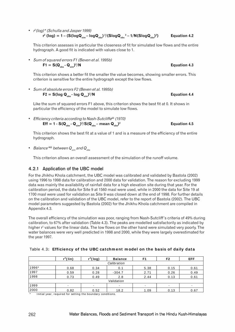
The overall efficiency of the simulation was poor, ranging from Nash-Sutcliff’s criteria of 49% duringcalibration, to 67% after validation (Table 4.3). The peaks are modelled satisfactorily as indicated byhigher r2 values for the linear data. The low flows on the other hand were simulated very poorly. Thewater balances were very well predicted in 1998 and 2000, while they were largely overestimated forthe year 1997.

Table 4.3: Efficiency of the UBC catchment model on the basis of daily data

r2(lin) r2(log) Balance F1 F2 EFF Calibration

1996* 0.68 0.34 0.1 5.38 0.15 0.61 1997 0.59 0.28 -304.7 2.71 0.26 0.49 1998 0.73 0.49 2.8 2.44 0.13 0.61

Validation 1999 - - - - - - 2000 0.82 0.52 18.2 1.09 0.13 0.67 * Initial year, required for setting the boundary conditions.


The model could simulate a good fit in the case of monthly flow (Figure 4.4) and flow duration curves(Figure 4.5), while the statistical characteristics of the observed time series were conserved by thesimulated time series. The mean discharge of the observed data series was 1.57 m3/s. This wasslightly overestimated by UBC at a value of 1.76 m3/s. The standard deviation ranged from 2.35 m3/sin the case of the simulated time series to 2.68 m3/s for the observed data series. Both time seriesobserved a similar range with 31.0 m3/s in the case of the observed time series and 31.4 m3/s for thesimulated time series. An overall correlation coefficient of 0.78 was observed between the two timeseries. A visual comparison of the two time series shows that the recession curves, particularly inthe years 1996 and 1997, are inadequately simulated (Figure 4.6).

The monthly discharge shown in Figure4.4 shows, in general, a good fit with theexception of 1997. The overall correlationcoefficient for monthly flow between thesimulated and the observed time serieswas 0.90. The linear trend line comparingthe two time series follows the ideal linewith a regression coefficient of 0.81. In1997, the monthly flow was overestimatedby the model during the monsoon seasonand underestimated during the winter andpre-monsoon seasons.

The duration curve is very well simulatedwith a correlation coefficient of 0.99between the observed and the simulatedtime series (Figure 4.5). The linear trendline follows the ideal line closely with aregression coefficient of 0.98. The flows ofhigher exceedance probability are, ingeneral, well simulated up to about 7 m3/s.Above this the values are generallyunderestimated up to about 15 m3/s. Thehigh flows are randomly estimated withgood fits, underestimated, oroverestimated values.

a) Monthly mean discharge

0

1

2

3

4

5

6

7

Jan-96 Sep-96 May-97 Jan-98 Sep-98 Jun-99 Feb-00 Oct-00

Mea

n m

onth

ly d

isch

arge

[m3 /s

]

Simulated Observed

b) Comparison of simulated and observed monthly discharge

y = 0.8526x + 0.0888R2 = 0.8056

0

1

2

3

4

5

6

0 1 2 3 4 5 6 7

Simulated discharge [m3/s]

Obs

erve

d di

scha

rge

[m3 /s

]

Figure 4.4: Monthly mean discharMonthly mean discharMonthly mean discharMonthly mean discharMonthly mean discharge on the basis of observed and simulated flows using the UBCge on the basis of observed and simulated flows using the UBCge on the basis of observed and simulated flows using the UBCge on the basis of observed and simulated flows using the UBCge on the basis of observed and simulated flows using the UBCmodel: a) monthly mean discharmodel: a) monthly mean discharmodel: a) monthly mean discharmodel: a) monthly mean discharmodel: a) monthly mean discharge, b) comparison of monthly mean discharge, b) comparison of monthly mean discharge, b) comparison of monthly mean discharge, b) comparison of monthly mean discharge, b) comparison of monthly mean dischargegegegege

a) Duration curves

0

5

10

15

20

25

30

35

0 20 40 60 80 100Probability [%]

Dai

ly d

isch

arge

[m3 /s

]

Deficit Sim Deficit Obs Exceedance Sim Exceedance Obs

b) Comparison between simulated and observed duration curve

y = 1.1726x - 0.0839R2 = 0.9804

0

5

10

15

20

25

30

35

40

0 5 10 15 20 25 30 35


Obs

erve

d di

scha

rge

[m3 /s

]

Figure 4.5: Observed and simulated duration curveObserved and simulated duration curveObserved and simulated duration curveObserved and simulated duration curveObserved and simulated duration curveusing UBC model: a) duration curves of exceedanceusing UBC model: a) duration curves of exceedanceusing UBC model: a) duration curves of exceedanceusing UBC model: a) duration curves of exceedanceusing UBC model: a) duration curves of exceedanceand deficit, b) comparison between observed andand deficit, b) comparison between observed andand deficit, b) comparison between observed andand deficit, b) comparison between observed andand deficit, b) comparison between observed andsimulated curvessimulated curvessimulated curvessimulated curvessimulated curves


4.2.1.1 Remarks on the use of the model

The UBC model shows the largest advantages in catchments with a small number of rainfallstations. As Bastola (2002) mentions, this advantage is offset in the case of the Jhikhu Kholacatchment with the large number and rather well-distributed rainfall sites. The very restrictive datainput format and the calibration of the UBC model are demanding of time and labour. Improvementsin the model’s efficiency can be achieved mainly by better discharge data sets, particularly in thelow flow regime.

4.2.2 Application of the Tank model

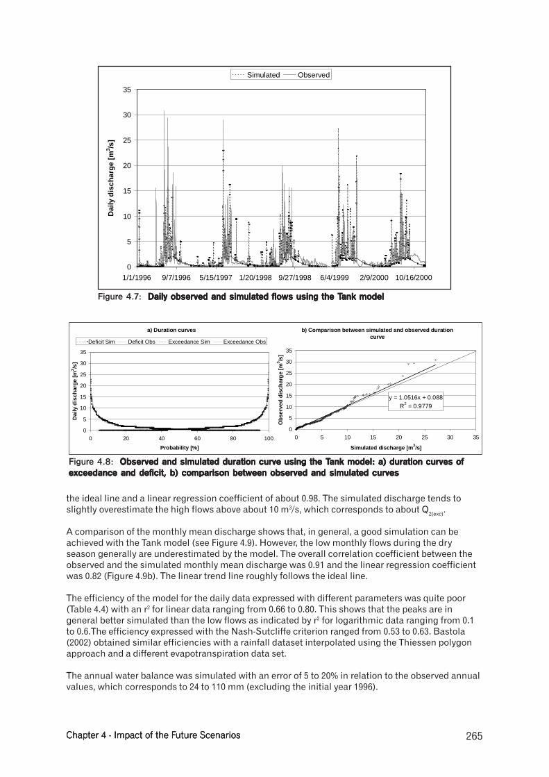
The Tank model was calibrated using the genetic optimisation algorithm implemented in the Tankmodel version 1.0.0 coded by Bastola et al. (2002) on the basis of the tournament selection process.The input data consisted of the daily precipitation interpolated using the interpolation module ofWaSim-ETH (Schulla and Jasper 1999), monthly reference evapotranspiration calculated accordingto the FAO-Penman-Monteith method (FAO 1998), and the daily observed discharge at Site 1 of theJhikhu Khola catchment. The model parameters suggested after the calibration and used in thevalidation of the model are shown in Appendix 4.4. For a first comparison of the observed andsimulated flows using this model, refer to Figure 4.7, the daily observed and simulated flows.

The statistical characteristics of the observed hydrograph were preserved by the simulatedhydrograph. A mean of 1.57 m3/s was calculated for the observed discharge, while the mean of thesimulated discharge was 1.41m3/s. The standard deviation was 2.62 m3/s for the observed dischargeand 2.47 m3/s for the simulated discharge. The range was about 30 m3/s in the observed dischargeand 27 m3/s in the simulated discharge. The overall correlation coefficient between observed andsimulated discharge was 0.78. These values roughly correspond with the values proposed by Bastola(2002) who used a different rainfall input series as well as a different evapotranspiration input series.

The qualitative comparison of the simulated and observed discharges on a daily basis shows thatthe simulated peaks are generally lower than the observed peaks. The simulated recession curvesafter the monsoon season reach the low base flows later than the observed recession curves. Inaddition, the simulated hydrograph is smoother than the observed hydrograph.

The comparison of the duration curves (Figure 4.8) shows that, in general, the model was able tosimulate the duration curve rather well. An overall correlation coefficient between the observed andthe simulated duration curve of 0.99 was achieved with a linear trend line approximately following

Figure 4.6: Daily observed and simulated flows using the UBC modelDaily observed and simulated flows using the UBC modelDaily observed and simulated flows using the UBC modelDaily observed and simulated flows using the UBC modelDaily observed and simulated flows using the UBC model

0

5

10

15

20

25

30

35

1/1/1996 12/31/1996 12/31/1997 12/31/1998 12/31/1999 12/30/2000

Dai

ly d

isch

arge

[m3 /s

]

Simulated Observed


the ideal line and a linear regression coefficient of about 0.98. The simulated discharge tends toslightly overestimate the high flows above about 10 m3/s, which corresponds to about Q

2(exc).

A comparison of the monthly mean discharge shows that, in general, a good simulation can beachieved with the Tank model (see Figure 4.9). However, the low monthly flows during the dryseason generally are underestimated by the model. The overall correlation coefficient between theobserved and the simulated monthly mean discharge was 0.91 and the linear regression coefficientwas 0.82 (Figure 4.9b). The linear trend line roughly follows the ideal line.

The efficiency of the model for the daily data expressed with different parameters was quite poor(Table 4.4) with an r2 for linear data ranging from 0.66 to 0.80. This shows that the peaks are ingeneral better simulated than the low flows as indicated by r2 for logarithmic data ranging from 0.1to 0.6.The efficiency expressed with the Nash-Sutcliffe criterion ranged from 0.53 to 0.63. Bastola(2002) obtained similar efficiencies with a rainfall dataset interpolated using the Thiessen polygonapproach and a different evapotranspiration data set.

The annual water balance was simulated with an error of 5 to 20% in relation to the observed annualvalues, which corresponds to 24 to 110 mm (excluding the initial year 1996).

0

5

10

15

20

25

30

35

1/1/1996 9/7/1996 5/15/1997 1/20/1998 9/27/1998 6/4/1999 2/9/2000 10/16/2000

Dai

ly d

isch

arge

[m3 /s

]

Simulated Observed

Figure 4.7: Daily observed and simulated flows using the TDaily observed and simulated flows using the TDaily observed and simulated flows using the TDaily observed and simulated flows using the TDaily observed and simulated flows using the Tank modelank modelank modelank modelank model

a) Duration curves

0

5

10

15

20

25

30

35

0 20 40 60 80 100

Probability [%]

Dai

ly d

isch

arge

[m3 /s

]



y = 1.0516x + 0.088R2 = 0.9779

0

5

10

15

20

25

30

35

0 5 10 15 20 25 30 35


Obs

erve

d di

scha

rge

[m3 /s

]

Figure 4.8: Observed and simulated duration curve using the TObserved and simulated duration curve using the TObserved and simulated duration curve using the TObserved and simulated duration curve using the TObserved and simulated duration curve using the Tank model: a) duration curves ofank model: a) duration curves ofank model: a) duration curves ofank model: a) duration curves ofank model: a) duration curves ofexceedance and deficit, b) comparison between observed and simulated curvesexceedance and deficit, b) comparison between observed and simulated curvesexceedance and deficit, b) comparison between observed and simulated curvesexceedance and deficit, b) comparison between observed and simulated curvesexceedance and deficit, b) comparison between observed and simulated curves


The validation period from 1999 to 2000 showed comparable values with the calibration period from1996 to 1998.


A major advantage of this model is the simple data input format, the low input data requirements, aswell as the fast and simple calibration process through the application of the genetic algorithm. Thesimplicity in terms of data input, however, is on the cost of the use of this model for studies relatedto land-use change. The model does not allow the input of catchment characteristics as they are notrequired to run this model, but are necessary for land-use change studies. For the application ofclimate scenarios, however, this model can be used.

The low efficiency of the model is assumed to be a direct cause of the quality of the discharge data,mainly in terms of low flows. The differences in peak discharge can probably be attributed to thetemporal resolution of the data. Most discharge events and herein the peaks of these events onlylast for a few hours and are often the direct cause of heavy rainfall intensities. In the temporalresolution of one day, this effect is not properly reflected. The efficiency of this model couldpresumably be enhanced with improved discharge data quality as well as with more adequateevapotranspiration input data.

4.2.3 Application of PREVAH model

4.2.3.1 Data preparation

The spatial data requirements of PREVAH are quite extensive. Besides the digital elevation model(DEM) it requires land-use and a number of soil parameters (Table 4.5). In the case of the JhikhuKhola catchment, a DEM was generated from the 1:20,000 map with contours of 50 m equidistance(Integrated Survey Section 1989). The land-use maps (*.pus and *.use) were prepared from the1:20,000 land-use map produced from 1996 aerial photos with detailed ground verification by BhubanShrestha, PARDYP, Nepal. Soil depth information for the entire catchment was derived from the

Table 4.4: Efficiency of the Tank model on the basis of daily data

r2(lin) r2(log) F1 F2 Balance Nash-Sutcliffe

Calibration 1996* 0.66 -0.30 5.79 0.30 167.2 0.58

1997 0.69 0.57 2.04 0.16 -65.2 0.61

1998 0.71 0.43 2.57 0.15 102.6 0.58

Validation

1999 0.67 0.42 2.67 0.50 -24.1 0.53

2000 0.80 0.09 1.21 0.25 113.1 0.63 * Initial year, required for setting the boundary conditions


0

1

2

3

4

5

6

Jan-96 Sep-96 May-97 Jan-98 Sep-98 Jun-99 Feb-00 Oct-00

Mea

n m

onth

ly d

isch

arge

[m3 /s

]

Sim Obs


y = 0.8694x + 0.3557R2 = 0.8265

0

1

2

3

4

5

6

0 1 2 3 4 5 6


Obs

erve

d di

scha

rge

[m3 /s

]

Figure 4.9: Monthly mean discharMonthly mean discharMonthly mean discharMonthly mean discharMonthly mean discharge on the basis of observed and simulated flows using the Tge on the basis of observed and simulated flows using the Tge on the basis of observed and simulated flows using the Tge on the basis of observed and simulated flows using the Tge on the basis of observed and simulated flows using the Tankankankankankmodel: a) monthly mean discharmodel: a) monthly mean discharmodel: a) monthly mean discharmodel: a) monthly mean discharmodel: a) monthly mean discharge, b) comparison of monthly mean discharge, b) comparison of monthly mean discharge, b) comparison of monthly mean discharge, b) comparison of monthly mean discharge, b) comparison of monthly mean dischargegegegege


sediment source survey (MRE 2002). The remaining soil parameters were estimated from measuredand mapped texture during the land systems’ mapping (Maharjan 1991) using the soil texturetriangle by Saxton et al. (1986). All base maps were provided as grids of 50 m*50 m cell size.

The meteorological input data consisted of the daily precipitation data of 10 sites and the dailytemperature data of 9 sites in the Jhikhu Khola catchment. Additionally, the daily rainfall data fromNagarkot (DHM 2000) were used as there are no stations in the western and upper parts of thecatchment at present. For calibration the daily streamflow data at the outlet of the Jhikhu Kholacatchment at Site 1 were used.

The Jhikhu Khola catchment consists of 44,429 grid cells of the size 50 m*50 m. This is on the basisof the DEM generated catchment area of 111.1 km2. The entire catchment was classified into 14height zones with a range of 100 m, ranging from 800 to 2200 m, five aspect classes (NW-NE, NE-SE,SE-SW, SW-NW, flat), four slope classes (0-10, 10-22, 22-36, >36), and five classes each for soiltopographic and area topographic index. On the basis of these classes, 1163 hydrotopes weregenerated using the criteria height zone (intersected with catchment ID), exposition, land use, andsoil-topographic index.

4.2.3.2 Model calibration and validation

Although a number of parameters required for the model can be extracted from the catchmentcharacteristics imported with the spatial data as discussed above, a number of other parametershave to be calibrated using the measured discharge as a reference. These parameters are compiledin Table 4.6 with the resulting values after the calibration and validation. For this purpose, the year1996 as initial year and the years 1997 and 1998 as calibration years were chosen (see also above).The efficiency results achieved through this process are compiled in Table 4.7.

Table 4.5: Input data information for the application of the PREVAH model

Catchment Jhikhu Khola Period for calibration 1996-1998 Period for validation 1999-2000 Spatial input data ([unit]; PREVAH file extension)

- elevation ([m]; *.dhm) - land use/cover ([PREVAH categories]#; *.use) - land use/cover ([PREVAH categories]; *.pus) - soil depth ([m]; *.btk) - soil depth ([class]; *.pat) - soil depth ([class]; *.art) - available field capacity ([vol%]; *.pfc) - saturated hydraulic conductivity ([mm/h]; *.kwt) - saturated hydraulic conductivity ([m/s]; *.kms)

Spatial resolution 50 m * 50 m cell size --> 44,429 cells Meteorological input data - precipitation of 11 sites

- temperature of 9 sites Discharge data - discharge of Site 1 main hydro station Temporal resolution of input data 1 day # For PREVAH categories refer to Zappa (1999)

Table 4.6: Parameters calibrated for the PREVAH model

Value Parameter Description 0.0 PKORF correction for rain [%] 0.8 CREDV reduction factor for open and vegetated land 0.4 CBETA exponent, soil moisture recharge parameter 0.1 Cu relative part of field capacity below which EA<ET0 0.6 CRSZ maximum portion 2 SGRLUZ threshold content of SUZ for generation of surface runoff [mm] 5 K0H storage time for fast runoff R0 [h] 100 K1H storage time for delayed runoff R1 [h] 1500 K2H storage time for slow runoff R2 [h] 700 CG1H storage time for fast baseflow R [h] 0.0 SLZ1MAX storage capacity for fast baseflow R [mm] 0.9 CPERC infiltration intensity [mm/h]


The balance is simulated by PREVAH, with errors ranging from 1 to 25% with reference to theobserved values. This corresponds to absolute errors of between 8 and 150 mm per year. The balanceis very accurately predicted in the validation period. Overall, the efficiency of the modelling usingPREVAH on a daily time basis is satisfactory but far from good. In all years a Nash-Sutcliffeefficiency of more than 0.50 was achieved with a peak of 0.71 in 1997. The peaks are generallysimulated better than the low flows, as shown with higher r2 values for linear data than r2 values forlogarithmic data.

A qualitative comparison of the daily flows shows that the general recession trend is picked upnicely by the model, but in general the model reaches the low baseflows later than the observeddischarge (see also Figure 4.10). In addition to this, the peaks are generally underestimated by themodel, which is also shown with a lower range for simulated discharge. While the range for theobserved data set is about 30 m3/s, it is only 26 m3/s for the simulated data set. The simulated timeseries preserves the statistical characteristics of the observed time series. The mean of the observeddischarge is 1.57 m3/s. The simulated discharge mean is 1.46 m3/s. Standard deviations are 2.62 and2.47 m3/s for the observed and the simulated time series, respectively. The overall correlationcoefficient between the simulated and observed data series is 0.80.

Overall, the mean monthly discharge (Figure 4.11a) shows a generally good fit. This is not onlyshown visually, but also with an overall correlation coefficient between the observed and thesimulated monthly time series of 0.91 and a linear regression, which roughly follows an ideal line(Figure 4.11 b), with a regression coefficient of 0.83. The visual comparison shows a majordiscrepancy in the monsoon flows of 2000, otherwise it shows a good fit (Figure 4.11a).

Table 4.7: Assessment of performance of the PREVAH model

r2(lin) r2(log) Balance F1 F2 EFF Calibration

1996* 0.70 -1.73 5.06 0.63 80.5 0.63 1997 0.76 0.67 1.55 0.12 -44.6 0.71 1998 0.72 0.55 2.52 0.12 146.7 0.59

Validation 1999 0.75 0.44 2.06 0.43 19.4 0.64 2000 0.73 0.45 1.66 0.15 -8.0 0.50 * initial year, required for setting the boundary conditions

Figure 4.10: Observed and simulated daily discharObserved and simulated daily discharObserved and simulated daily discharObserved and simulated daily discharObserved and simulated daily discharge at the main station, Jhikhu Khola catchmentge at the main station, Jhikhu Khola catchmentge at the main station, Jhikhu Khola catchmentge at the main station, Jhikhu Khola catchmentge at the main station, Jhikhu Khola catchment

0

5

10

15

20

25

30

35

1/1/1996 7/19/1996 2/4/1997 8/23/1997 3/11/1998 9/27/1998 4/15/1999 11/1/1999 5/19/2000 12/5/2000

Dis

char

ge [m

3 /s]

Simulated Observed


The comparison of the duration curve (Figure 4.12) shows a nearly identical match between theobserved and the simulated data series. The correlation coefficient between the duration curves ofthe two time series is 0.99. The linear regression shows nearly the same direction and position asthe ideal line and has a regression coefficient of 0.99. The fit can be observed up to about 20 m3/s.Only the four biggest events do not fit.

A comparison of the annual simulated evapotranspiration values at the potential rates with the arielevapotranspiration rates, calculated according to the FAO (1998) method, showed that the simulatedevapotranspiration rates are, in general, about 5% lower than the calculated rates. The actualevapotranspiration rates differ by about 20% on an annual basis. This suggests that more attentionmust be given to this part of the water balance.


The PREVAH model has extensive data requirements and is therefore quite labour intensive. Notonly the data preparation, but also the calibration process is time consuming. In terms of efficiency,a number of improvements can be made. These include the following.

• Currently the precipitation is imported on the basis of daily data (if daily data are modelled). This

daily data are then converted to four equal rainfall amounts distributed equally throughout theday. This however does not take into consideration the large dependency on rainfall intensity orthe particular daily rainfall distribution.

• Evapotranspiration in this application of PREVAH was calculated using the approach of Hamon

(1961), which only requires temperature data. For better results, other approaches implemented inPREVAH should be used. The measurement network in the Jhikhu Khola has been upgradedaccordingly, with relative humidity loggers at all sites and the installation of an automaticweather station additionally monitoring solar radiation and wind.


0

1

2

3

4

5

6

Jan-96 May-97 Sep-98 Feb-00

Mea

n m

onth

ly d

isch

arge

[m3 /s

]

Simulated Observed


y = 0.8265x + 0.3779R2 = 0.829

0

1

2

3

4

5

6

0 1 2 3 4 5 6


Obs

erve

d di

scha

rge

[m3 /s

]

Figure 4.11: Observed and simulated (PREVObserved and simulated (PREVObserved and simulated (PREVObserved and simulated (PREVObserved and simulated (PREVAH) monthly mean discharAH) monthly mean discharAH) monthly mean discharAH) monthly mean discharAH) monthly mean discharge at the main station of thege at the main station of thege at the main station of thege at the main station of thege at the main station of theJhikhu Khola catchment: a) mean monthly discharJhikhu Khola catchment: a) mean monthly discharJhikhu Khola catchment: a) mean monthly discharJhikhu Khola catchment: a) mean monthly discharJhikhu Khola catchment: a) mean monthly discharge, b) comparison of mean monthly discharge, b) comparison of mean monthly discharge, b) comparison of mean monthly discharge, b) comparison of mean monthly discharge, b) comparison of mean monthly dischargegegegege

a) Duration curves

0

5

10

15

20

25

30

35

0 20 40 60 80 100

Probability [%]

Dai

ly d

isch

arge

[m3 /s

]



y = 1.056x + 0.0241R2 = 0.9864

0

5

10

15

20

25

30

35

0 5 10 15 20 25 30 35


Obs

erve

d di

scha

rge

[m3 /s

]

Figure 4.12: Observed and simulated (PREVObserved and simulated (PREVObserved and simulated (PREVObserved and simulated (PREVObserved and simulated (PREVAH) duration curves at the main station of the JhikhuAH) duration curves at the main station of the JhikhuAH) duration curves at the main station of the JhikhuAH) duration curves at the main station of the JhikhuAH) duration curves at the main station of the JhikhuKhola catchment: a) duration curves, b) comparison of duration curvesKhola catchment: a) duration curves, b) comparison of duration curvesKhola catchment: a) duration curves, b) comparison of duration curvesKhola catchment: a) duration curves, b) comparison of duration curvesKhola catchment: a) duration curves, b) comparison of duration curves


• The vegetation parameters were used according to the data sets implemented. It is

acknowledged that the vegetation parameters for this agricultural system as well as for theprevalent forests in this region do not match. Due to the lack of the respective information, thiswas however necessary. In recent years, the Integrated Pest Management Project assessed anumber of the necessary vegetation parameters, which will probably be available later this year(Herrmann, pers. comm.). The large differences in calculated and simulated actualevapotranspiration rates could herewith presumably be reduced.

4.2.4 Comparison of the models

In general, it has been seen that all models show rather low efficiencies. The low flows in particulartend to be modelled inefficiently, which generally is the easier part in a modelling exercise. In thissection the performance of the three models will be compared. With respect to all the efficiencyparameters compared, the PREVAH model showed, on average, the best performance (Table 4.8).This is followed by the Tank model and finally the UBC model. In terms of time and labour demand,the Tank model shows the best performance with its simple data input format and the implementedgenetic algorithm. In terms of data requirements, the PREVAH model is most demanding and is alsovery labour intensive. However, this model shows the most scope for further improvement with theaddition of a number of meteorological parameters as well as site-specific vegetation parameters.Additionally, improved discharge data quality would lead to an improved efficiency of this model.The efficiency of the other models can only be enhanced with improved discharge data quality.

In Figure 4.13 the outputs of the different models are compared. While the simulated baseflows ofthe Tank and the PREVAH models are very similar, the baseflows of the UBC model are generallyoverestimated. It is important to note that all models show inadequate fit of the recession curvesafter the monsoon season. While the observed dataset immediately recedes to the low flow levels,the simulated results approach the low base flows more gently.

The most similar results are produced bythe PREVAH and Tank model shown withthe regression line in Figure 4.13a with aregression coefficient of 0.92 and acorrelation coefficient of 0.95 (Table 4.9).The correlation coefficient between theobserved data sets and the PREVAH modeloutput is likewise the highest at 0.80.

The similar behaviour of the three models interms of output efficiency suggests that the main limitations have to be sought in the input data set.With the problems of data collection and rating curve establishment as discussed in Appendix A3.1,the main reason has to be the discharge data set.

For further studies and to improve the efficiency of the models, the project should strive for moreaccurate discharge information mainly in the low flow season (see also Chapter 6). In addition, theimpact of the numerous irrigation diversions have to be taken into consideration and further studiedin detail.

Table 4.8: Efficiency parameters compared between the three models

UBC Tank PREVAH r2(lin) r2(log) Balance EFF r2(lin) r2(log) Balance EFF r2(lin) r2(log) Balance EFF

1997 0.59 0.28 -304.7 0.49 0.69 0.57 -65.2 0.61 0.76 0.67 -44.6 0.71 1998 0.73 0.49 2.8 0.61 0.71 0.43 102.6 0.58 0.72 0.55 146.7 0.59 1999 - - - - 0.67 0.42 -24.1 0.53 0.75 0.44 19.4 0.64 2000 0.82 0.52 18.2 0.67 0.80 0.09 113.1 0.63 0.73 0.45 -8.0 0.50

Mean 0.71 0.43 108.6 0.59 0.72 0.38 76.3 0.59 0.74 0.53 54.7 0.61

Table 4.9: Correlation matrix for daily discharge simulated with different models

Qobs QUBC QTank QPREVAH

Qobs 1.00 0.78 0.78 0.80

QUBC 1.00 0.93 0.90

QTank 1.00 0.95

QPREVAH 1.00


In terms of the models’ use for the scenarios below, the PREVAH model can be applied both to theclimate as well as to the land-use scenario. The remaining models, UBC and Tank, can only beapplied to the climate scenario as land use/cover has no impact on the Tank model and only limitedimpact in the case of the UBC model through the percentage of forest cover and impermeable areas.For the sake of simplicity only the two models, PREVAH with the best performance and the Tankmodel with the easiest handling, were used for the scenario analyses.

4.3 SCENARIOS

A number of external driving forces are responsible for changing water supply and demandscenarios and the change in flood and land-degradation susceptibilities. Schultz (2000) mentionsclimate change, economic restrictions, ecological restrictions, land-use change, and differencesources of pollution which all have an impact on future water supply. Water demand, according tothe same author, shows a major impact as a result of climate change, population growth, changingstandards of living, and industrial development. The main external driving forces in the context ofthe middle mountains in Nepal are considered to be the climate, the population, the economicconditions, and national and district policies (see also Chapter 1). In this respect, three mainscenarios were parameterised to assess their impact on the state of the water resources in theselected catchments. These scenarios do not represent a complete set of possible futuredevelopment, but should show simple examples for the PARDYP Water and Erosion Studies whichcould be incorporated in the near future for the temporal as well as for the spatial up-scalingexercise proposed in Phase 3 (ICIMOD 2003).

The main questions to be answered below were as follows.

• How can the given scenarios be parameterisd for a middle mountain catchment in the HKH?

• What is the potential impact of the scenarios identified on indicators relevant to water availability,

flooding, and land degradation?

a) Hydrographs

0

5

10

15

20

25

30

35

1/1/1997 10/28/1997 8/24/1998 6/20/1999 4/15/2000

Dai

ly d

isch

arge

[m3 /s

]

QUBC QTank QPREVAH

c) UBC vs. Tank

y = 0.9275x - 0.27R2 = 0.8583

0

5

10

15

20

25

30

35

0 5 10 15 20 25 30 35

Discharge QUBC [m3/s]

Dis

char

ge Q

Tank

[m3 /s

]b) UBC vs. PREVAH

y = 0.8958x - 0.1625R2 = 0.806

0

5

10

15

20

25

30

35

0 5 10 15 20 25 30 35

Discharge QUBC [m3/s]

Dis

char

ge Q

PREV

AH [m

3 /s]

d) Tank vs. PREVAH

y = 0.9218x + 0.1208R2 = 0.9151

0

5

10

15

20

25

30

0 5 10 15 20 25 30

Discharge QTank [m3/s]

Dis

char

ge Q

PREV

AH [m

3 /s]

Figure 4.13: Comparison of simulated daily discharComparison of simulated daily discharComparison of simulated daily discharComparison of simulated daily discharComparison of simulated daily discharge of UBC, Tge of UBC, Tge of UBC, Tge of UBC, Tge of UBC, Tank, and PREVank, and PREVank, and PREVank, and PREVank, and PREVAH modelsAH modelsAH modelsAH modelsAH models


4.3.1 Scenario 1: Climate Change

Climate change is one of the most publicised issues in recent decades. A large number of studiesinto the reasons, impacts, and scenarios of climate change have been undertaken in this time. Avery good source for mainstream information on this issue is provided by the IntergovernmentalPanel on Climate Change (IPCC). Most of the information below is therefore based on the work ofIPCC.

Surface temperature change in the last 100 years ranged from 0.3 to 0.8 °C in the region of TropicalAsia, including the South Asian countries (IPCC 1998). According to the same report, the projectedtemperature changes for the entire globe between 1990 and 2100 are likely to be in the range of 1.5 to4.5 °C. For South Asia an above average temperature increase is predicted (Figure 4.14). An evenhigher increase is foreseen for the Tibetan plateau. Lal (2002) suggests an increase in temperature of3.5 to 5.5 °C by the end of 2100 of the land regions of the Indian sub-continent. For Nepal, Arun B.Shrestha noted an increase of 0.06 °C per year in the average temperature (Kathmandu Post 2003).

Chalise (1994) stresses the importance of understanding the possible impacts of climate change asthis will add to the already existing uncertainties of widespread environmental degradation in theregion. This author further discusses some possible signs of climate change on the basis of:

• noontime temperature distribution in Kathmandu, which shows a slight increase over recent

years;and

• glacier fluctuations in the region, which generally indicate a retreating trend and therefore a

warming of the atmosphere.

For tropical Asia, IPCC (1998) suggests an impact on water resources as follows.

• The Himalayas play a critical role in the provision of water to continental monsoon Asia.

• Increased temperature and increased seasonal variability in precipitation are expected to result in

accelerated recession of glaciers and increasing danger from glacial lake outburst floods.

• A reduction in the flow of snow and ice-fed rivers, accompanied by increases in peak flows and

sediment yields, would have major impacts on hydropower regeneration, urban water supply, andagriculture.

Figure 4.14: Change in temperatur Change in temperatur Change in temperatur Change in temperatur Change in temperature re re re re relative to model’s global mean elative to model’s global mean elative to model’s global mean elative to model’s global mean elative to model’s global mean (from IPCC 1998)


• Availability of water from snow-fed rivers may increase in the short term, as glaciers recede, but

decrease in the long term.

• Runoff from rain-fed rivers may change in the future. A reduction in snowmelt water would result

in decreases in the dry-season flow of these rivers.

• Large populations and increasing demands in the agricultural, industrial, and hydropower sectors

will put additional stress on water resources.

• Pressure will be most acute on drier river basins and those subject to low seasonal flows.

Recently, the focus of global climate change discussions has been on the type of precipitation, andin particular the proportion of precipitation, that falls as snow. Amongst others, Harrison et al. (2001)studied climate change and its impact on the snowfall pattern in Scotland. It is important to notethat global climate change not only has negative impacts. Positive impacts could also be envisaged,such as longer growing seasons for higher altitudes.

Lal (2002) projects for the Indiansub-continent decreasing rainfallin winter and increasing rainfallduring the monsoon (Table 4.10).A decrease of 10 to 20% in winteris simulated by 2050. During themonsoon an increase of 30% ormore in precipitation over India is projected. Lal (2002) further suggests that the variability in themonsoon’s onset will increase. However, there is conflicting information on the basis of differentGCMs (global climate models). Lal et al. (1995) found a decline in mean summer monsoon rainfall ofabout 0.5 mm/day over the South Asian region. This decline in summer monsoon rainfall has alsobeen suggested by some experiments referred to in IPCC (1998).

The changes in temperature and in precipitation are expected to have a major impact on theavailability of water resources in the region. For the meso-scale catchments, the expected primaryimpact of this scenario as presented in Table 0.10 may show the following impact chain:

1) increase in temperature during dry season months/decrease in precipitation → increasedevapotranspiration rates → faster reduction of seasonal soil moisture and groundwater storage →reduced groundwater and spring yield → reduced runoff → increased pressure on waterresources;and

2) increase in precipitation during the monsoon season months → increased runoff → increasedsusceptibility to floods and land degradation caused by water.

The disaggregated scenario with different values for the winter and monsoon was calculated usingthe models Tank and PREVAH.

4.3.2 Scenario 2: Population

Population has been increasing tremendously in the Indian sub-continent. Many authors cautionfrom further increase and project a collapse of the natural resource base in case of furtherpopulation stress (e.g. Allen 2000). Other authors argue that, with increasing population, the peoplewould introduce innovative management technologies and practices to cope with the worseningresource situation (Paudel and Thapa 2001). There is, however, no argument that more people needmore water and more food.

In Nepal, the annual population growth rate for the eco-regional zone of the hills was calculated at2% for the period between 1991 and 2001 (MOPE 2002). The annual population growth rate for theJhikhu Khola catchment was assessed to be 3.1% for the period from 1947 to 1990 and 3.5% between1947 and 1996. While these growth rates are important parameters, they are not very useful for long-term projections. For this purpose, a number of additional parameters such as fertility rate, numberof births, number of deaths, and migration rates are required. These parameters are not available forthe Jhikhu Khola catchment, therefore two population projections by Lutz and Goujon (2002) were

Table 4.10: Climate change parameters (by 2080)

Scenario Temperature Precipitation Reference - annual +5.6 °C +9.9 % - winter +6.3 °C -25 % - monsoon +4.6 °C +15 %

Lal (2002)


used (Table 4.11). The two projections a1b1 and a2 were used for the emission estimates of the IPCCSpecial Report on Emission Scenarios (Nakicenovic and Swart 2000) as lower and upper estimatesfor the world’s population. The projections firstly produced regional datasets for 13 world regions,which were then disaggregated to country level.

The projection a1b1 shows a low fertility/low mortality/central migration scenario and projects aworld population of 8.7 billion in 2055, which decreases to 7.1 billion in 2100 (IIASA 1999). Theprojection a1 represents a high fertility/high mortality/central migration scenario and projects aworld population of about 15 billion at the end of the 21st century. The disaggregated data for thecountry level of Nepal forecasts a population of about 36,000,000 in the case of the a1b1 scenarioand about 63,000,000 in the case of the a1 scenario by 2080. The population growth rates for theentire kingdom were used for the estimation of the population in the Jhikhu Khola.

It is further assumed that the people in the future will aspire to higher living standards and thereforeuse more water, e.g., for flush toilets (Verma et al. in prep). In addition to the population parametersa low, medium, and high water demand scenario was calculated and compared with the availablewater resources on the basis of existing as well as predicted water resources. The water demandvalues are based on the current water demand in the Jhikhu Khola catchment (Merz et al. 2002) inthe case of the low water demand, and projected for medium and high water demands based onGleick (1996). The basic water demand standard as proposed by Gleick (1996) is composed of 5 l/dayfor drinking, 20 l/day for sanitation, 15 l/day for bathing, and 10 l/day for cooking, all values perperson. For the high domestic water demand, this basic water demand was doubled.

Expected primary impact of this scenario:

Increased population → increased demand for domestic water → increased demand for food(intensification of land use is hardly possible on the basis of the present intensities. Expansion isdiscussed as an impact on land use in scenario 3).

4.3.3 Scenario 3: Land-use change due to poverty and landflucht (migration from theland)

Land-use change may have a major impact on the water resources, at the micro- to meso-scale inparticular (FAO 2002). As shown above, there is no clear evidence for a major land use shift atpresent in the catchments. However, as indicated in Chapter 2 and on the basis of the populationprojections, a change in land use could be well be possible. For future developments two differentpotential sub-scenarios were identified:

Landflucht (outmigration of people from rural to urban areas; urbanisation from the perspective ofthe rural areas)

In general, a trend towards increased urbanisation can be observed in Nepal and many othercountries of South Asia (UNFPA 2001). The urban growth rate in Nepal for the period 2000-2005 isprojected to be 5.1% (UNFPA 2001). In 2001, 14% of Nepal’s population lived in urban centres(MOPE 2002). This process affects the rural population. Urban migration is also the reason for ahigh percentage of migrants in Nepal (K.C. et al. 1998).

Table 4.11: Population and water demand parameters (by 2080)

Parameter Value Remarks Reference Population projection a1b1 196 % of the

population in 1990 low fertility/low mortality/central migration

Lutz and Goujon (2002)

Population projection a2 344 % of the population in 1990

high fertility/high mortality/central migration

Lutz and Goujon (2002)

Low domestic water demand 20l person-1day-1 current water demand in the Jhikhu Khola catchment

Merz et al. (2002)

Medium domestic water demand

50l person-1day-1 basic water demand Gleick (1996)

High domestic water demand 100l person-1day-1 double the basic water demand above


In the Jhikhu Khola catchment, a number of fields are not being cultivated as their owners live inKathmandu and have not given the land for tenancy. Often these owners have left their parentalhome for higher education or jobs in the capital or abroad. At the time of the parents death, or ifthe parents follow them to the city, the land remains uncultivated. Another reason for abandoningthe land is the low economic return from many fields, in particular in the upper catchment areas.It is not likely that abandoned land will be taken over by another family, as the return is toomarginal. Another reason for outmigration is poverty (Adhikari and Bohle 1999), although thesepeople often do not leave large plots of land behind and therefore do not contribute to land-usechange due to outmigration.

In terms of spatial distribution of the land, the most likely land to be abandoned is in the upperelevation areas. These are the marginal lands with steep slopes, often low soil fertility, and a hightendency towards soil erosion. The rainfed land on the border to the irrigated lands is more fertileand easier to cultivate due to accessibility and favourable slope. These lands would readily betaken over by other farmers in case of outmigration by the owners.

Expansion to marginal lands

Increasing population pressure and the need for cultivated land is believed to cause an expansion tomarginal and less suitable land (UNEP 2001). This process occurred in Nepal during the 1970s andwas the basis of the Theory of Himalayan Environmental Degradation (Eckholm 1970; Ives andMesserli 1989). However, many of the marginal areas on steep slopes have now been protected byinclusion into community forestry areas. For this reason, the community forestry regulations wereincorporated in the scenarios and only shrub and grassland were subject to potential change toagricultural land (Table 4.12). It is acknowledged that some of these areas have also been includedin the community forest areas as shown in Table 4.13, but in general these areas are small andnegligible at the catchment scale.

On the basis of these two sub-scenarios the parameters compiled in Table 4.12 were determined.Expected primary impacts of this scenario:1) Landflucht → increased area of grassland → increased flood volume and more frequent peaks

or

2) Expansion to marginal areas → increased area of cultivated land → decreased flood volume andreduced number of peaks.

This scenario was only calculated by using the PREVAH model.

Table 4.12: Land-use change parameters (by 2080)

Scenario Remarks Landflucht 1(L1) – High rate of abandoning

All the rainfed land above 1250 masl is abandoned and becomes grassland

Landflucht 2 (L2) – Medium rate of abandoning

All the rainfed land above 1500 masl is abandoned and becomes grassland

Expansion 1(E1) – High rate of expansion

All shrub and grasslands below 1250 masl are newly cultivated and become rainfed agricultural land

Expansion 2 (E2) – Low rate of expansion

All shrub and grasslands below 1500 masl are newly cultivated and become rainfed agricultural land

Table 4.13: Community forest areas in the Jhikhu Khola catchment (based on unpublished data by Bhuban Shrestha/PARDYP Nepal; all figures in km2)

Rainfed land Forest Grass Shrub Other Total in the catchment 42.7 33.2 6.1 7.8 3.3 Protected by community forest 1.2 11.8 0.4 0.9 0.2


4.4 IMPACT ASSESSMENT

The impact assessment of the scenarios described above should show preliminary results ofpossible analyses to be further pursued and investigated in more detail in the PARDYP framework.For the calculation of the scenarios, the data of 1996 to 1999 was used as a base (Table 4.2). Resultsfrom 1996 were omitted as these data were used to set the boundary conditions, e.g., the soilmoisture content or the groundwater.

4.4.1 Scenario 1: Climate change

The PREVAH and Tank models were used to assess the potential impact of a global climate changescenario as discussed above. The scenario was assessed on the basis of the data of 1997 to 1999.Overall, it can be observed that on a seasonal basis the runoff is considered to increase for themonsoon season and to decrease in the remaining seasons, particularly in the pre-monsoon season(Figure 4.15).

On the basis of the PREVAH model, potential evapotranspiration will increase by about 40% from1990 to 2080 if the climate change scenario occurs. The actual evapotranspiration rates wouldchange by about 10% on an annual basis. As these figures are still very preliminary due to theinappropriate vegetation datasets, no further disaggregation into different months or seasons ispresented here, although this would be of particular interest for the different areas in the catchment.

Comparing the duration curves for the data in the 1990s with the predicted values on the basis of theclimate scenario for the 2080s, no difference can be observed by applying the PREVAH model(Figure 4.16a). Using the Tank model on the other hand, the slope of the regression line has a slopegreater than 1, which indicates that significantly higher discharge values are expected on the basisof this model’s predictions (Figure 4.16b). The uncertainty shown by the results indicates that basingstream flows on the past data records may be inappropriate in future as the conditions may change.Great care will have to be taken in the design of structures.

a) PREVAH

-500

50100150200250300350400

Pre Mon Post Win Pre Mon Post Win Pre Mon Post Win

1997/2087 1998/2088 1999/2089

Run

off [

mm

]

1990s 2080s Simulated change

b) Tank

-500

50100150200250300350400

Pre Mon Post Win Pre Mon Post Win Pre Mon Post Win

1997/2087 1998/2088 1999/2089

Run

off [

mm

]


Figure 4.15: Seasonal changes with global climate change applying a) PREVSeasonal changes with global climate change applying a) PREVSeasonal changes with global climate change applying a) PREVSeasonal changes with global climate change applying a) PREVSeasonal changes with global climate change applying a) PREVAH model, b) TAH model, b) TAH model, b) TAH model, b) TAH model, b) Tankankankankankmodelmodelmodelmodelmodel

a) PREVAH model

y = 1.0085x - 0.0914R2 = 0.9985

0

5

10

15

20

25

30

0 5 10 15 20 25 30

Discharge 1990s [m3/s]

Dis

char

ge 2

080s

[m3 /s

]

b) Tank model

y = 1.1293x - 0.0979R2 = 0.9976

0

5

10

15

20

25

0 5 10 15 20 25

Discharge 1990s [m3/s]

Dis

char

ge 2

080s

[m3 /s

]

Figure 4.16: Comparison of duration curves for 1990s and 2080s using a) PREVComparison of duration curves for 1990s and 2080s using a) PREVComparison of duration curves for 1990s and 2080s using a) PREVComparison of duration curves for 1990s and 2080s using a) PREVComparison of duration curves for 1990s and 2080s using a) PREVAH model, b) TAH model, b) TAH model, b) TAH model, b) TAH model, b) Tankankankankankmodelmodelmodelmodelmodel


In terms of flood peaks, an increase in the number of peaks above 10 m3/s daily discharge isexpected on the basis of both models (Table 4.14). The simulated change in the number of peaks isgreater in the case of the Tank model than the PREVAH model. It should be noted that the numberof peaks observed is closer to the number of peaks estimated by the PREVAH model in the 1990sthan the number of peaks simulated by the Tank model.

In 1997, 6 peaks were observed; in 1998, 8 were seen; and in 1999, another 6. In addition, thePREVAH model shows slightly better fits for the high flows than the Tank model (see above in Table4.8). Summarised, with a global climate change according to IPCC (1998) and changes intemperature/precipitation in South Asia according to Lal (2002):

• evapotranspiration rates are expected to increase;

• water availability during the dry season can be expected to decrease;

• water volume during the monsoon can be expected to increase;

• number of flood peaks can be expected to increase; and

• design flows based on the past data records may show underestimated flows.

4.4.2 Scenario 2: Population growth

On the basis of the two populationprojections by Lutz and Goujon(2002) and the three water demandclasses of low, medium, and high-water demand, on the basis of thecurrent water requirements and thebasic domestic water requirementsaccording to Gleick (1996), thefollowing predictions can be madefor the water requirements in theJhikhu Khola catchment by 2080(see also Table 4.15):

• population in the catchment will be between about 85,000 and 150,000;

• this corresponds to a population density of 750 to 1400 people per km2;and

• annual water demand will range from 5 to 50 mm depending on the different water demand

scenarios.

The disaggregated information according to the VDCs in the Jhikhu Khola catchment shows thatthe highest increases in water demand are expected in the VDCs along the Arniko highway andsoon also along the Dhulikhel – Bardibas highway where the population is concentrated (Figure4.17). In 1996, the water demand in all VDCs was between 0 -6 mm. In case of a low daily waterdemand the VDCs Panchkhal, Patlekhet, Rabi Opi, Dhulikhel, and Phoolbari would show an annualwater demand of about 6 -12 mm in the case of a low population growth rate according to scenarioa1b1. In case of a high population growth rate as predicted by scenario a2, the same VDCs wouldexperience a water demand of about 12 -18 mm per annum. The remaining VDCs are expected tohave a water demand of 6 -12 mm per annum. In securing the basic water requirements, the water

Table 4.14: Number of peaks > 10 m3/s for 1990s and 2080s with different models


Year PREVAH Tank PREVAH Tank PREVAH Tank 1997/2087 4 2 5 5 +1 +3

1998/2088 3 2 3 2 0 0

1999/2089 7 7 8 11 +1 +4

Table 4.15: Projected population and water demand Jhikhu Khola catchment, 2080

Population Scenario a1b1 Scenario b2 Population 85,646 150,238 Population density [people/km2] 769 1349 Water demand Low daily demand [mm] 5.6 9.8 Medium daily demand [mm] 14.0 24.6 High daily demand [mm] 28.1 49.2


south-facing slopes plus Baluwa would be expected to show about 25-50 mm water demand and theremaining VDCs 50-75 mm. Comparing these values with the annual precipitation values or even themonthly precipitation values, there seems no problem of adequate water availability for domesticpurposes. However, in this context it has to be remembered that people generally do not userainwater, but surface water or shallow groundwater for domestic purposes. In this respect, anincrease in pollution as was observed in the Jhikhu Khola and documented by Merz et al. (2003b),would put further pressure on the available water resources. In addition, as was mentioned above,the agricultural water demand is more significant.

With the current very high level of agricultural intensity in the catchment (see Chapter 2), onlyexpansion to more marginal lands is possible (see Scenario 3 E1 and E2) if the catchment is toremain self-sufficient in staple food production and still be able to produce cash crops for themarkets in the city.

The following summary can be made.

• Water demand for domestic purposes will increase many times over with population growth.

• The main increase in water demand is not expected from population growth, but from increased

water demand to achieve a basic water supply according to Gleick’s (1996) figures.

• The main water demand increase in the Jhikhu Khola catchment is expected in the VDCs along

the two highways crossing the catchment. The VDCs in the upper part will have an importantfunction as recharge areas and water supply for the lower VDCs. This stresses the importance oflocal-level planning and management of the water resources at the catchment level.

4.4.3 Scenario 3: Land-use change

The calculation of this scenario with the PREVAH model generated a number of open questions,mainly in relation to the observation presented in Chapter 3. In terms of land- use change, thescenarios as presented above result in the expected changes shown in Table 4.16. The scenariosrelated to Landflucht result in a decrease of rainfed agricultural land with an approximate 10 to 34%decrease depending on the scenario. Grassland increases by 74 to 235% in scenarios Landflucht 2(L2) and Landflucht (L1), respectively. No changes are expected in the area of shrub land due tograzing and cutting of grasses.

Scenarios Expansion 1 (E1) and 2 (E2) are expected to result in the increase of rainfed agriculturalland at 20 to 30% depending on the scenario. This is at the cost of grassland (- 60 to 90%) and shrubland (- 60 to 90%).

The impact of these land-use changes simulated with the PREVAH model yield only little change, asshown in Table 4.17. In general, the Landflucht scenarios reduce the runoff, while the expansionscenarios increase the runoff. These results are in strong contrast to the results observed on thebasis of event analyses presented in Section3.4. According to these results, catchment runoffincreases with an increasing proportion of grassland in the catchment and reduces with theproportion of agricultural land in the catchment. Here the opposite is observed, i.e., the runoffdecreases with the proportion of grassland and is the smallest for scenario L1. It is interesting tonote that the scenario L1 however shows the highest runoff during the monsoon season.

Comparing the maxima for the four years used for these calculations (Figure 4.18), in three out offour years the Landflucht scenarios, i.e., the scenarios with increased grazing areas, showed the

Table 4.16: Land-use changes on the basis of the land-use scenarios

Land use 1990s L1 L2 E2 E2 Rainfed agricultural land 680 ha 448 ha 607 ha 876 ha 822 ha -34 % -10 % +29 % +21 % Grassland 98 ha 329 ha 171 ha 10 ha 37 ha +235 % +74 % -90 % -62 % Shrub land 125 ha 125 ha 125 ha 16 ha 44 ha ±0 % ±0 % -87 % -65 %


Figure 4.18: Comparison of maximaComparison of maximaComparison of maximaComparison of maximaComparison of maxima

0

5

10

15

20

25

30

7 8 9 10

Dis

char

ge [m

3 /s]

1990s 2080s_L1 2080s_L2 2080s_E1 2080s_E2

Table 4.17: Comparison of the PREVAH outputs with scenarios Landflucht 1 and 2 and Expansion 1 and 2 [all values in mm]

Season 1990s 2080s_L1 2080s_L2 2080s_E1 2080s_E2

Pre 27.0 26.1 26.7 27.6 27.5

Mon 291.1 291.6 291.1 291.4 291.2

Post 61.4 60.9 61.1 62.0 61.8

Win 26.9 26.4 26.7 27.3 27.2

Annual 406.4 405.0 405.6 408.3 407.7

peak runoffs. The differences, however, are marginal between the calculated discharges. Theseresults confirm the findings in Chapter 3.4 on the basis of which grassland is decisive in floodgeneration and the size of a flood peak. For conclusive answers, the findings presented here are,however, not adequate and further improvements have to be made. It is believed that with theavailability of the local vegetation characteristics in particular these results will become moreconclusive.

4.4.4 Discussion

Three different scenarios were parameterised based on global climate change, populationdevelopment, and land-use change. In brief, it was indicated that potential climate change as well asexpected population development might lead to an overall decrease in water availability during thedry season. This is due to a decrease in precipitation during these months, which also has anegative impact on the runoff in the catchment. In addition, water demand is expected to increasemany times over on the basis of increased population as well has higher water demands per capita.However, overall, the water demand for domestic purposes is expected to be covered. Theparameterisation of agricultural water demand is difficult as the extent to which agriculture can beintensified further is unclear.

During the monsoon season more rain is expected, which leads to a higher susceptibility to floodgeneration and land degradation. Whether this increase in rainfall also leads to an increase inrainfall intensity and rainfall erosivity still has to be established. On the basis of observations in


terms of relationship between maximum rainfall intensity and rainfall amount shown in Section 3.4;and between erosivity (which is calculated on the basis of rainfall intensity; see also Section 3.1) andrainfall amount by Ramprasad et al. (2000; an increase of both these parameters will have to beexpected. This increase is further expected to lead to higher and more frequent peaks.

For improved results of the scenario analyses further efforts must be undertaken to improve theefficiency of the models as discussed above. The results of the land-use scenario calculation aspresented above are not satisfactory at present, mainly due to the inadequate parameterisation ofthe local vegetation.

4.4.5 Summary and Outlook

A number of models have been applied for different purposes in the HKH, a detailed comparisonwith the same datasets as WMO (1975) or WMO (1990) however is missing. The most comprehensivestudies undertaken by NIH further concluded that data availability is a major constraint for thesuccessful application of rainfall-runoff models in the mountainous regions. In general, distributedmodels seem to be more appropriate for mountainous conditions due to the highly variable andheterogeneous conditions in mountain areas, however, the data requirements are often notappropriate.

In this study, three different models were calibrated and validated, the UBC, the Tank model, and thePREVAH model. Of these models, PREVAH showed the best performance, although overall theefficiency for all models was quite low. The main reason for this is the quality of the discharge data,mainly in the low flow regime. In addition, the evapotranspiration in all cases had to be estimatedfrom temperature and none of the more sophisticated methods could be used. With theimprovements of the hydrological stations to increase their low flow sensitivity and additional datato calculate evapotranspiration the efficiency could be increased. In the case of the PREVAH modelthe use of local vegetation characteristics could further improve its efficiency.

The three scenarios based on global climate change, population growth coupled with increasingwater demand and rise in living standards, as well as land-use change— both abandoning ofmarginal land and expansion to marginal fields — showed that overall an increase in water demandhas to be expected from all sectors at a time where water availability from precipitation and fromrunoff during the dry season is presumably going to decrease, and during the wet season is going toincrease. This suggests that newly implemented water management options have to increasesupply, reduce demand, and enhance water quality. This was discussed in some detail in Merz et al.(2003c).

The use of models on PARDYP data has only just begun, but will receive further attention in the on-going Phase 3. After a model review, which will build on the first overview of model applications inthe region based on available literature, modelling exercises will be conducted in all catchments ofthe PARDYP network with the aim of predicting future developments and spatial up-scaling. In thiscontext it seems to be important to further investigate the impact of the numerous irrigationdiversions. Models like WaSim-ETH (Schulla 1997) provide the possibility of including irrigation inthe modelling exercise. Other models that could provide good results are expected to be the SLURPmodel, where there is the possibility of using remotely-sensed data, and which is fully based on landuse (Kite 1995); or the SWAT model (Arnold et al. 1998) implemented in an ArcView environment.The Chinese PARDYP team has first experiences with the VIC model, but have not yet produced anyconclusive results.

First initiatives towards a regional comparison of hydrological catchment and rainfall-runoff modelshave been made in the context of the HKH FRIEND project with the aim of conducting a regionalworkshop on hydrological modelling, followed by regional training on modelling and a regionalcomparison of different, promising models (Merz 2003).

The impact of these scenarios will be further discussed in Chapter 5 with the impact on theproposed indices.


SYNOPSIS 4: IMPACT OF FUTURE SCENARIOS

Hydrological models were used to document the potential impact of three scenariosbased on global climate change, population growth coupled with increased waterdemand to meet basic requirements, and local land-use change with expansion tomarginal lands or abandoning of marginal fields. The preliminary results for the JhikhuKhola catchment have revealed that:

• during the dry season water is becoming more scarce due to decreased

precipitation, increased evapotranspiration, and decreased runoff;

• flood events during the wet season are becoming more frequent and are of

marginally higher magnitude;and

• dependency of lower lying administrative units in a catchment on upper

administrative units is increasing due to the increase of water demand in theselower areas, which are generally more accessible and productive. This calls for theintroduction of catchment-based management of water resources.

These results suggest that more attention should be paid to the storage of surplus waterin the wet season to be used during the dry season, as seasonality will probably becomeeven more pronounced in future. While domestic water use is presently below basicwater requirements according to Gleick (1996), water supply should take intoconsideration both a change in population as well as in terms of daily water demands.This suggests that water management options of the future are to tap all availableresources, minimise losses and inefficiencies, and improve considerably the quality ofthe water.

Documents

Chapter 4: Impact of Future Scenarioslib.icimod.org/record/21652/files/c_attachment_103_1834.pdf · Chapter 4: Impact of Future Scenarios ... availability, flood generation potential,