Embed Size (px)
Citation preview
4.1
Chapter 4
Digital Transmission
4.2
4-1 DIGITAL-TO-DIGITAL CONVERSION
In this section, we see how we can represent digital
data by using digital signals. The conversion involves
three techniques: line coding, block coding, and
scrambling. Line coding is always needed; block
coding and scrambling may or may not be needed.
Line Coding
Line Coding Schemes
Block Coding
Scrambling
Topics discussed in this section:
4.3
Line Coding
Converting a string of 1’s and 0’s (digital data) into a sequence of signals that denote the 1’s and 0’s.
For example a high voltage level (+V) could represent a “1” and a low voltage level (0 or -V) could represent a “0”.
4.4
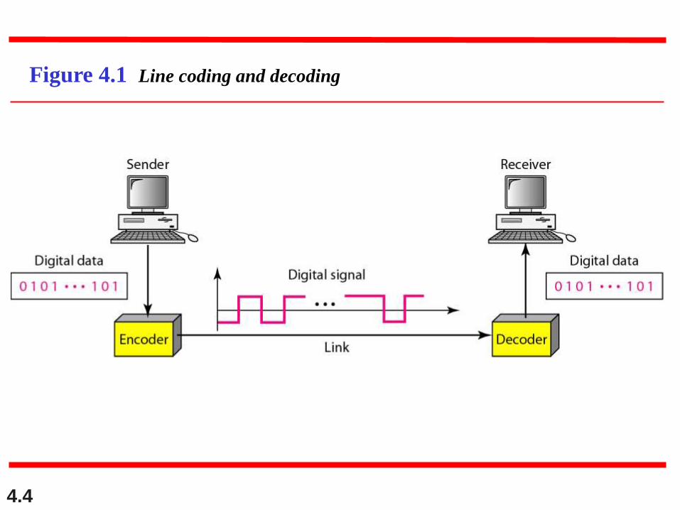
Figure 4.1 Line coding and decoding
4.5
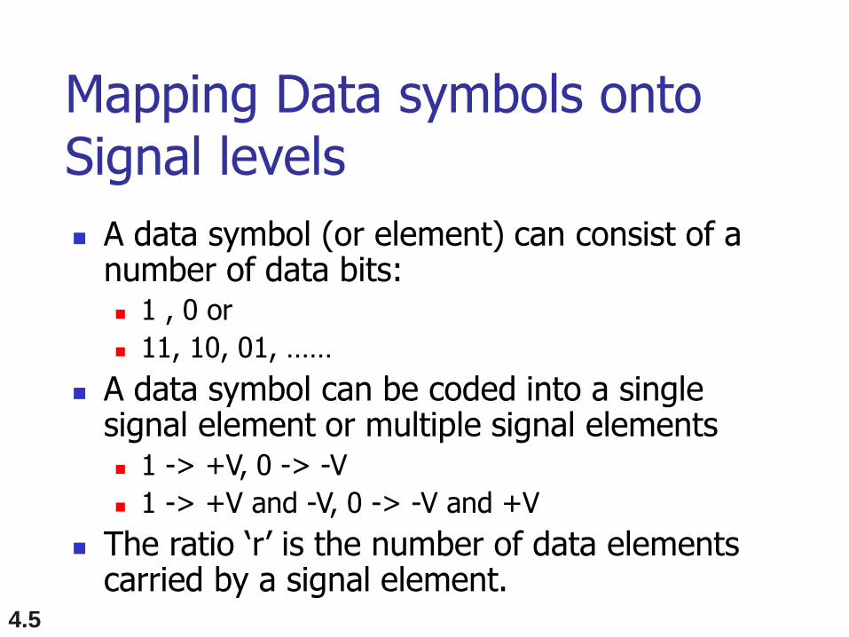
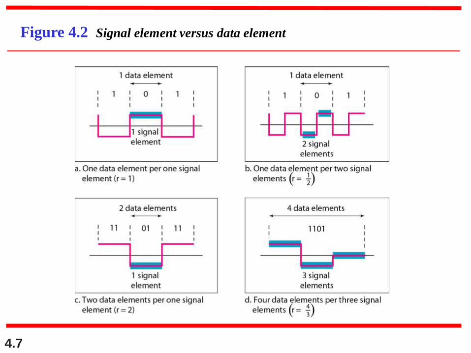
Mapping Data symbols onto Signal levels
A data symbol (or element) can consist of a number of data bits: 1 , 0 or
11, 10, 01, ……
A data symbol can be coded into a single signal element or multiple signal elements 1 -> +V, 0 -> -V
1 -> +V and -V, 0 -> -V and +V
The ratio ‘r’ is the number of data elements carried by a signal element.
4.6
Relationship between data rate and signal rate
The data rate defines the number of bits sent per sec - bps. It is often referred to the bit rate.
The signal rate is the number of signal elements sent in a second and is measured in bauds. It is also referred to as the modulation rate.
Goal is to increase the data rate whilst reducing the baud rate.
4.7
Figure 4.2 Signal element versus data element
4.8
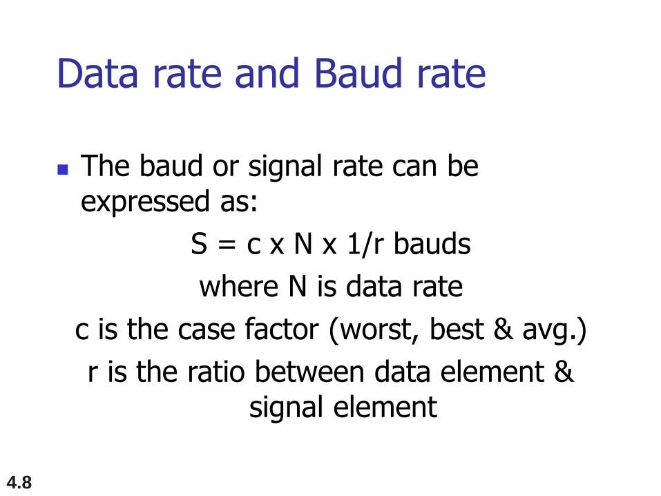
Data rate and Baud rate
The baud or signal rate can be expressed as:
S = c x N x 1/r bauds
where N is data rate
c is the case factor (worst, best & avg.)
r is the ratio between data element & signal element
4.9
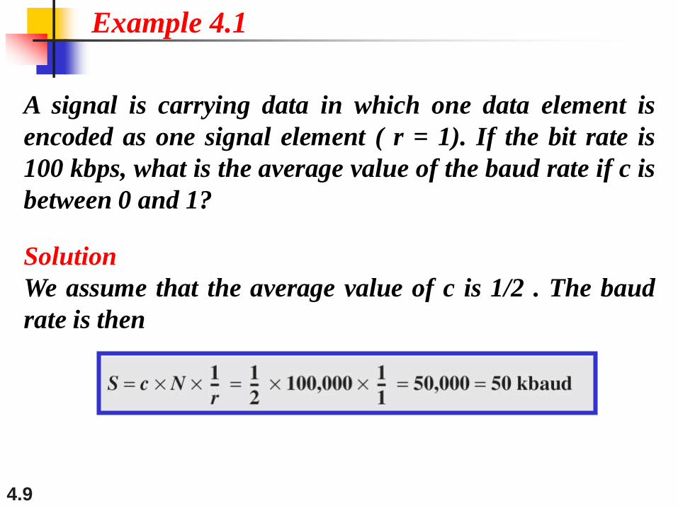
A signal is carrying data in which one data element is
encoded as one signal element ( r = 1). If the bit rate is
100 kbps, what is the average value of the baud rate if c is
between 0 and 1?
Solution
We assume that the average value of c is 1/2 . The baud
rate is then
Example 4.1
4.10
Although the actual bandwidth of a
digital signal is infinite, the effective
bandwidth is finite.
Note
4.11
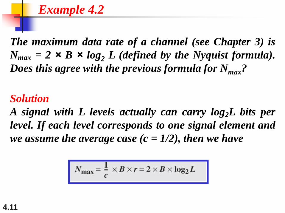
The maximum data rate of a channel (see Chapter 3) is
Nmax = 2 × B × log2 L (defined by the Nyquist formula).
Does this agree with the previous formula for Nmax?
Solution
A signal with L levels actually can carry log2L bits per
level. If each level corresponds to one signal element and
we assume the average case (c = 1/2), then we have
Example 4.2
4.12
Considerations for choosing a good signal element referred to as line encoding
Baseline wandering - a receiver will evaluate the average power of the received signal (called the baseline) and use that to determine the value of the incoming data elements. If the incoming signal does not vary over a long period of time, the baseline will drift and thus cause errors in detection of incoming data elements.
A good line encoding scheme will prevent long runs of fixed amplitude.
4.13
Line encoding C/Cs
DC components - when the voltage level remains constant for long periods of time, there is an increase in the low frequencies of the signal. Most channels are bandpass and may not support the low frequencies.
This will require the removal of the dc component of a transmitted signal.
4.14
Line encoding C/Cs
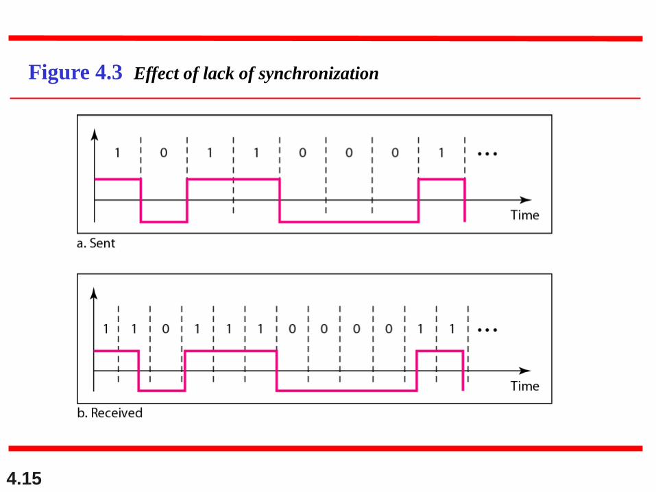
Self synchronization - the clocks at the sender and the receiver must have the same bit interval.
If the receiver clock is faster or slower it will misinterpret the incoming bit stream.
4.15
Figure 4.3 Effect of lack of synchronization
4.16
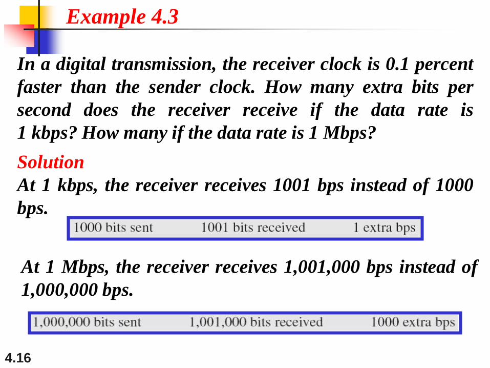
In a digital transmission, the receiver clock is 0.1 percent
faster than the sender clock. How many extra bits per
second does the receiver receive if the data rate is
1 kbps? How many if the data rate is 1 Mbps?
Solution
At 1 kbps, the receiver receives 1001 bps instead of 1000
bps.
Example 4.3
At 1 Mbps, the receiver receives 1,001,000 bps instead of
1,000,000 bps.
4.17
Line encoding C/Cs
Error detection - errors occur during transmission due to line impairments.
Some codes are constructed such that when an error occurs it can be detected. For example: a particular signal transition is not part of the code. When it occurs, the receiver will know that a symbol error has occurred.
4.18
Line encoding C/Cs
Noise and interference - there are line encoding techniques that make the transmitted signal “immune” to noise and interference.
This means that the signal cannot be corrupted, it is stronger than error detection.
4.19
Line encoding C/Cs
Complexity - the more robust and resilient the code, the more complex it is to implement and the price is often paid in baud rate or required bandwidth.
4.20
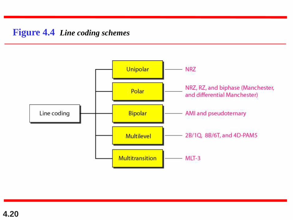
Figure 4.4 Line coding schemes
4.21
Unipolar
All signal levels are on one side of the time axis - either above or below
NRZ - Non Return to Zero scheme is an example of this code. The signal level does not return to zero during a symbol transmission.
Scheme is prone to baseline wandering and DC components. It has no synchronization or any error detection. It is simple but costly in power consumption.
4.22
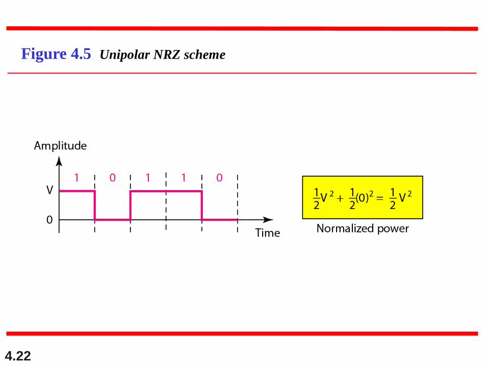
Figure 4.5 Unipolar NRZ scheme
4.23
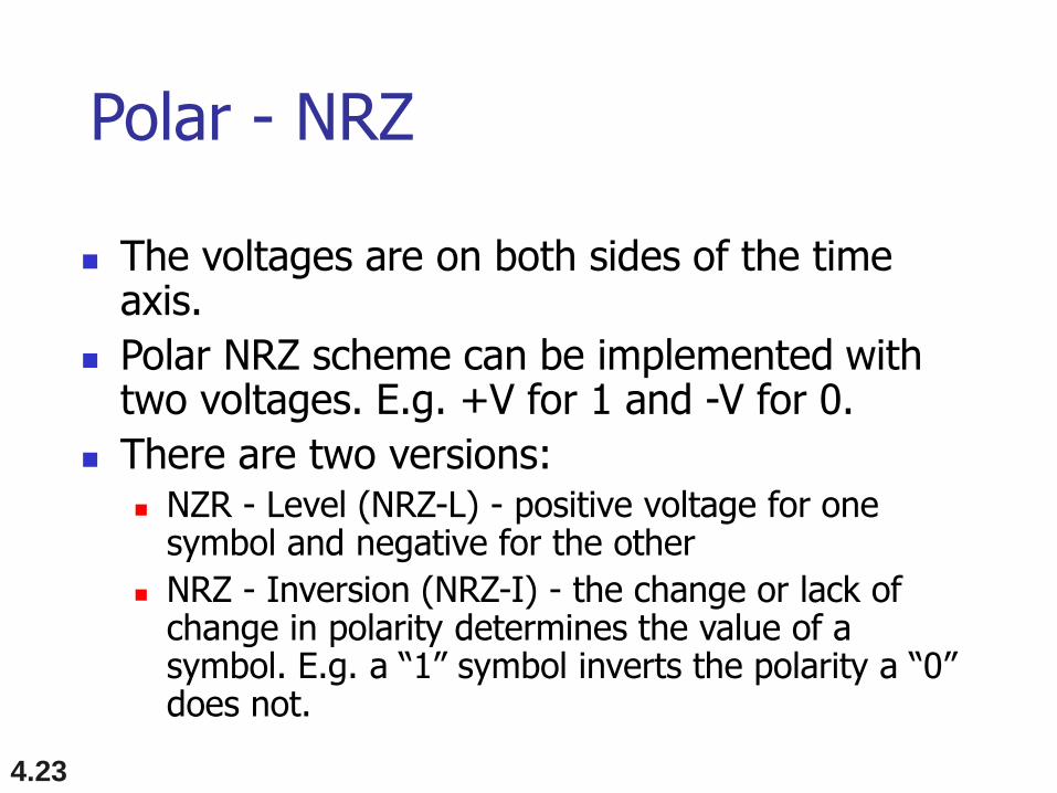
Polar - NRZ
The voltages are on both sides of the time axis.
Polar NRZ scheme can be implemented with two voltages. E.g. +V for 1 and -V for 0.
There are two versions: NZR - Level (NRZ-L) - positive voltage for one
symbol and negative for the other
NRZ - Inversion (NRZ-I) - the change or lack of change in polarity determines the value of a symbol. E.g. a “1” symbol inverts the polarity a “0” does not.
4.24
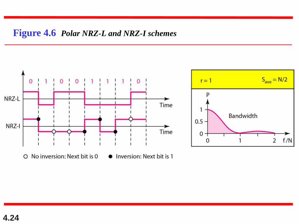
Figure 4.6 Polar NRZ-L and NRZ-I schemes
4.25
In NRZ-L the level of the voltage
determines the value of the bit.
In NRZ-I the inversion
or the lack of inversion
determines the value of the bit.
Note
4.26
NRZ-L and NRZ-I both have an average
signal rate of N/2 Bd.
Note
4.27
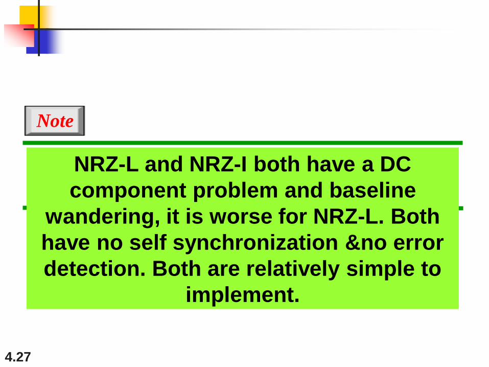
NRZ-L and NRZ-I both have a DC
component problem and baseline
wandering, it is worse for NRZ-L. Both
have no self synchronization &no error
detection. Both are relatively simple to
implement.
Note
4.28
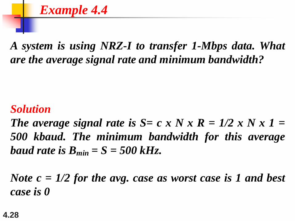
A system is using NRZ-I to transfer 1-Mbps data. What
are the average signal rate and minimum bandwidth?
Solution
The average signal rate is S= c x N x R = 1/2 x N x 1 =
500 kbaud. The minimum bandwidth for this average
baud rate is Bmin = S = 500 kHz.
Note c = 1/2 for the avg. case as worst case is 1 and best
case is 0
Example 4.4
4.29
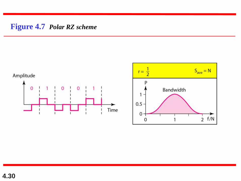
Polar - RZ The Return to Zero (RZ) scheme uses three
voltage values. +, 0, -.
Each symbol has a transition in the middle. Either from high to zero or from low to zero.
This scheme has more signal transitions (two per symbol) and therefore requires a wider bandwidth.
No DC components or baseline wandering.
Self synchronization - transition indicates symbol value.
More complex as it uses three voltage level. It has no error detection capability.
4.30
Figure 4.7 Polar RZ scheme
4.31
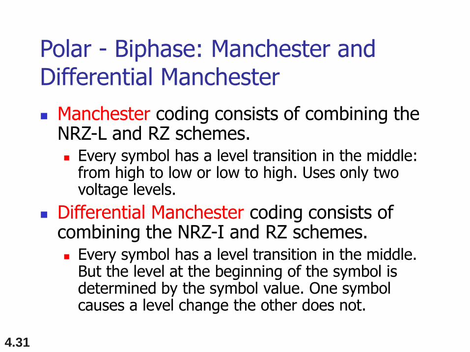
Polar - Biphase: Manchester and Differential Manchester
Manchester coding consists of combining the NRZ-L and RZ schemes. Every symbol has a level transition in the middle:
from high to low or low to high. Uses only two voltage levels.
Differential Manchester coding consists of combining the NRZ-I and RZ schemes. Every symbol has a level transition in the middle.
But the level at the beginning of the symbol is determined by the symbol value. One symbol causes a level change the other does not.
4.32
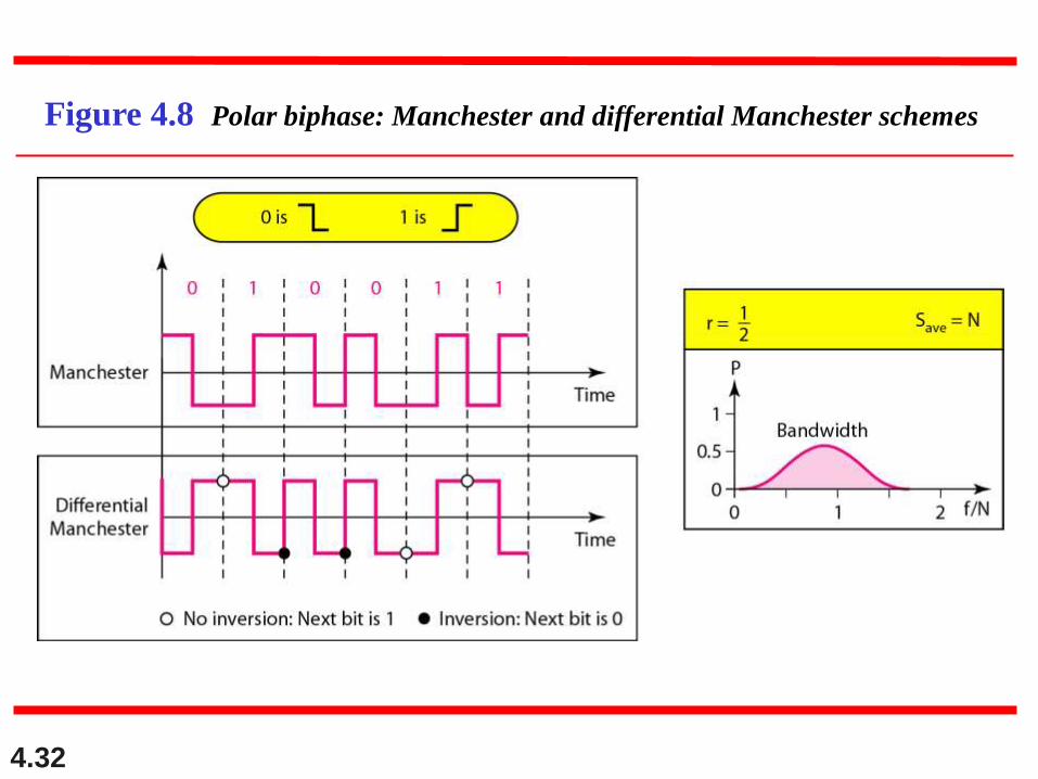
Figure 4.8 Polar biphase: Manchester and differential Manchester schemes
4.33
In Manchester and differential
Manchester encoding, the transition
at the middle of the bit is used for
synchronization.
Note
4.34
The minimum bandwidth of Manchester
and differential Manchester is 2 times
that of NRZ. The is no DC component
and no baseline wandering. None of
these codes has error detection.
Note
4.35
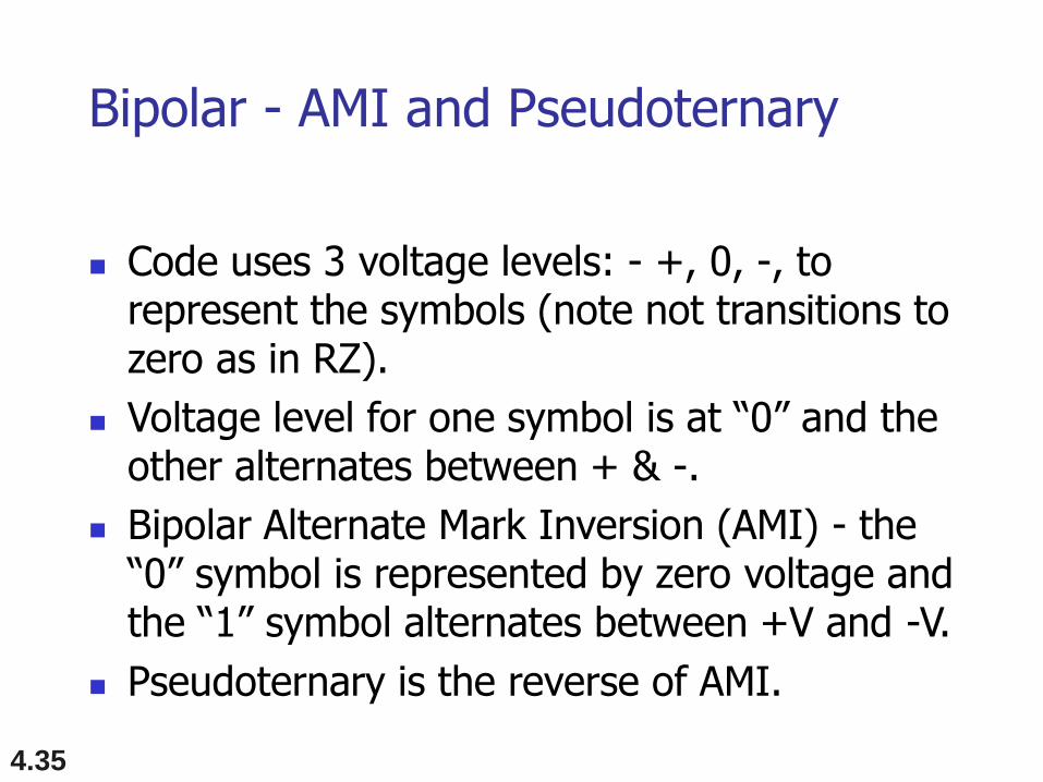
Bipolar - AMI and Pseudoternary
Code uses 3 voltage levels: - +, 0, -, to represent the symbols (note not transitions to zero as in RZ).
Voltage level for one symbol is at “0” and the other alternates between + & -.
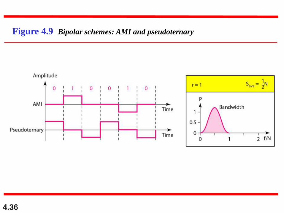
Bipolar Alternate Mark Inversion (AMI) - the “0” symbol is represented by zero voltage and the “1” symbol alternates between +V and -V.
Pseudoternary is the reverse of AMI.
4.36
Figure 4.9 Bipolar schemes: AMI and pseudoternary
4.37
Bipolar C/Cs
It is a better alternative to NRZ.
Has no DC component or baseline wandering.
Has no self synchronization because long runs of “0”s results in no signal transitions.
No error detection.
4.38
Multilevel Schemes
In these schemes we increase the number of data bits per symbol thereby increasing the bit rate.
Since we are dealing with binary data we only have 2 types of data element a 1 or a 0.
We can combine the 2 data elements into a pattern of “m” elements to create “2m” symbols.
If we have L signal levels, we can use “n” signal elements to create Ln signal elements.
4.39
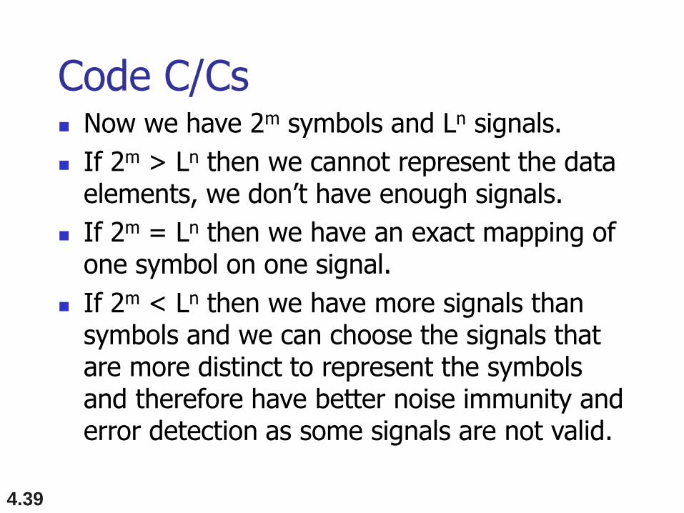
Code C/Cs Now we have 2m symbols and Ln signals.
If 2m > Ln then we cannot represent the data elements, we don’t have enough signals.
If 2m = Ln then we have an exact mapping of one symbol on one signal.
If 2m < Ln then we have more signals than symbols and we can choose the signals that are more distinct to represent the symbols and therefore have better noise immunity and error detection as some signals are not valid.
4.40
In mBnL schemes, a pattern of m data
elements is encoded as a pattern of n
signal elements in which 2m ≤ Ln.
Note
4.41
Representing Multilevel Codes
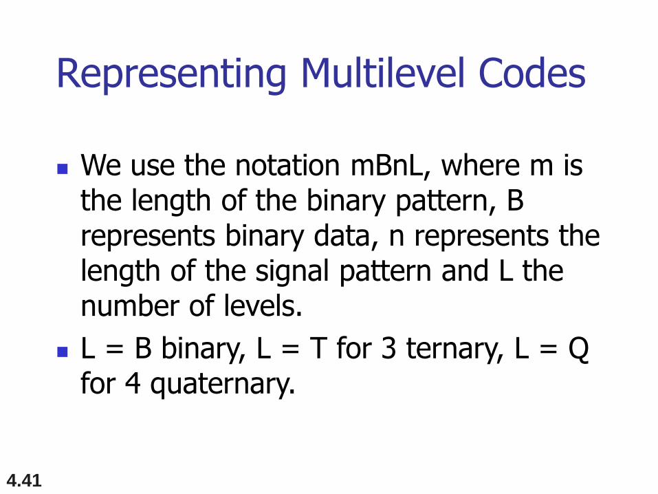
We use the notation mBnL, where m is the length of the binary pattern, B represents binary data, n represents the length of the signal pattern and L the number of levels.
L = B binary, L = T for 3 ternary, L = Q for 4 quaternary.
4.42
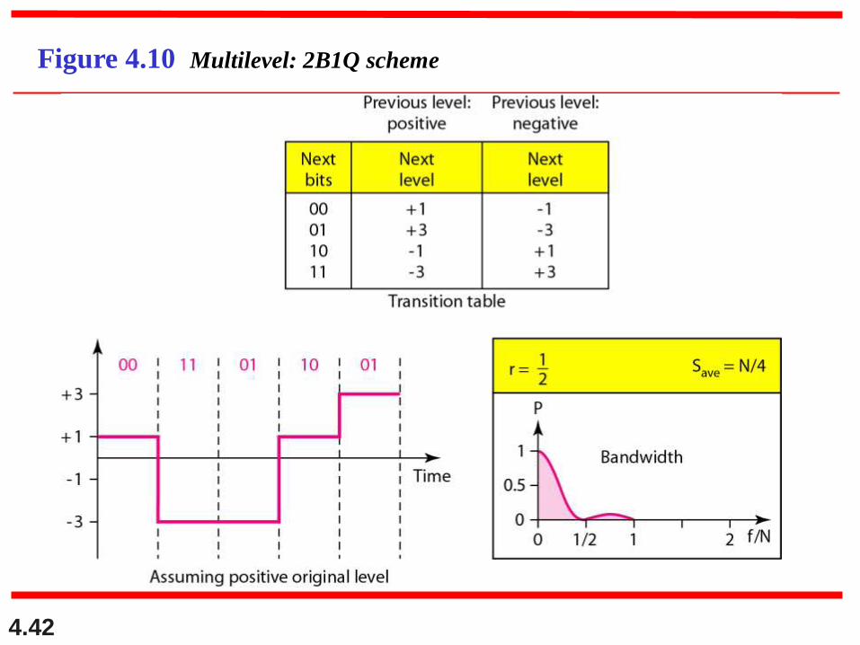
Figure 4.10 Multilevel: 2B1Q scheme
4.43
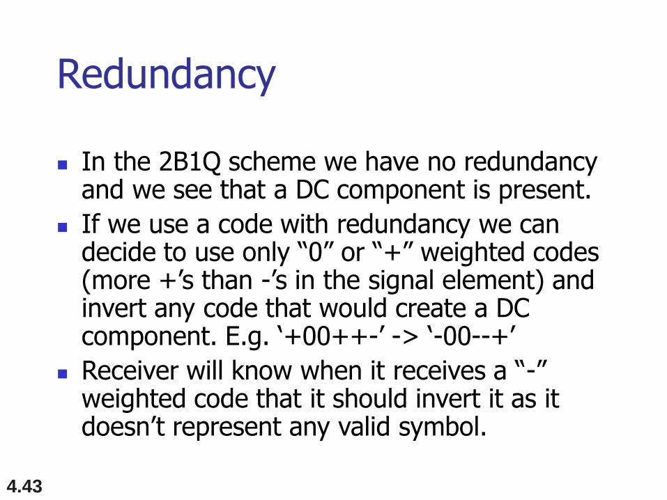
Redundancy
In the 2B1Q scheme we have no redundancy and we see that a DC component is present.
If we use a code with redundancy we can decide to use only “0” or “+” weighted codes (more +’s than -’s in the signal element) and invert any code that would create a DC component. E.g. ‘+00++-’ -> ‘-00--+’
Receiver will know when it receives a “-” weighted code that it should invert it as it doesn’t represent any valid symbol.
4.44
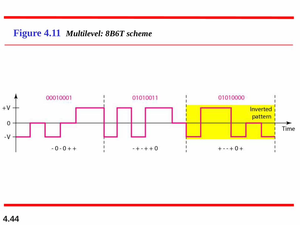
Figure 4.11 Multilevel: 8B6T scheme
4.45
Multilevel using multiple channels
In some cases, we split the signal transmission up and distribute it over several links.
The separate segments are transmitted simultaneously. This reduces the signalling rate per link -> lower bandwidth.
This requires all bits for a code to be stored.
xD: means that we use ‘x’ links
YYYz: We use ‘z’ levels of modulation where YYY represents the type of modulation (e.g. pulse ampl. mod. PAM).
Codes are represented as: xD-YYYz
4.46
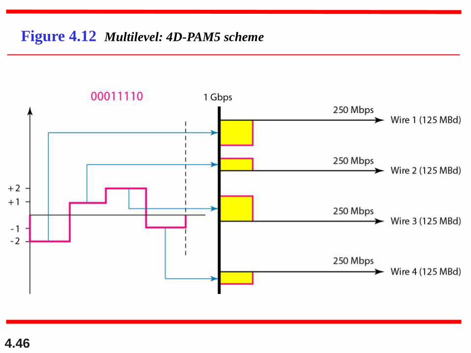
Figure 4.12 Multilevel: 4D-PAM5 scheme
4.47
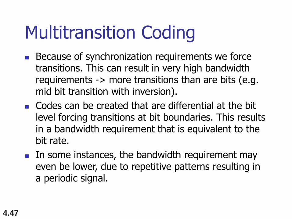
Multitransition Coding Because of synchronization requirements we force
transitions. This can result in very high bandwidth requirements -> more transitions than are bits (e.g. mid bit transition with inversion).
Codes can be created that are differential at the bit level forcing transitions at bit boundaries. This results in a bandwidth requirement that is equivalent to the bit rate.
In some instances, the bandwidth requirement may even be lower, due to repetitive patterns resulting in a periodic signal.
4.48
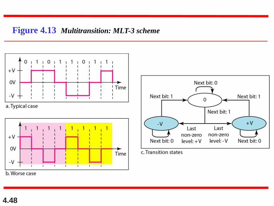
Figure 4.13 Multitransition: MLT-3 scheme
4.49
MLT-3
Signal rate is same as NRZ-I
But because of the resulting bit pattern, we have a periodic signal for worst case bit pattern: 1111
This can be approximated as an analog signal a frequency 1/4 the bit rate!
4.50
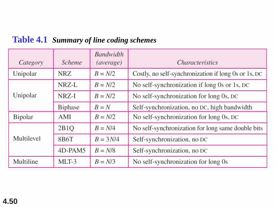
Table 4.1 Summary of line coding schemes
4.51
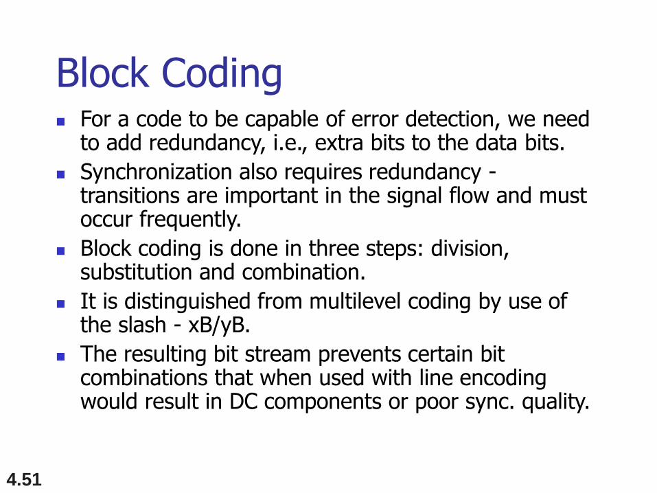
Block Coding For a code to be capable of error detection, we need
to add redundancy, i.e., extra bits to the data bits.
Synchronization also requires redundancy -transitions are important in the signal flow and must occur frequently.
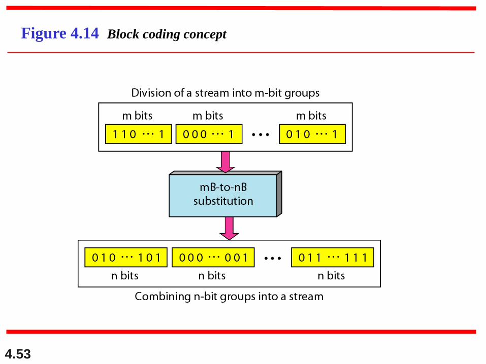
Block coding is done in three steps: division, substitution and combination.
It is distinguished from multilevel coding by use of the slash - xB/yB.
The resulting bit stream prevents certain bit combinations that when used with line encoding would result in DC components or poor sync. quality.
4.52
Block coding is normally referred to as
mB/nB coding;
it replaces each m-bit group with an
n-bit group.
Note
4.53
Figure 4.14 Block coding concept
4.54
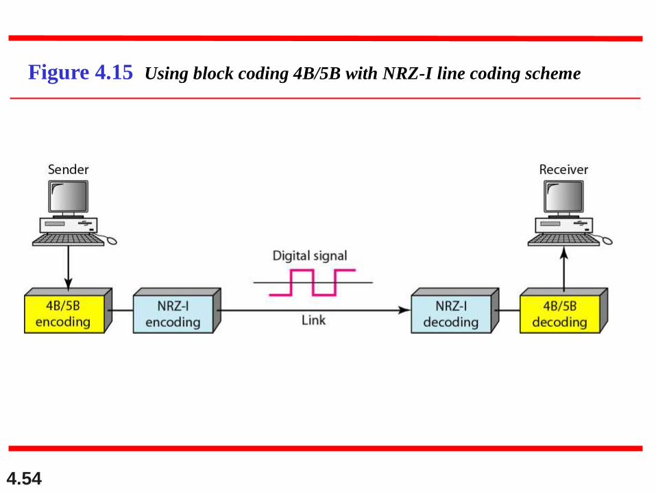
Figure 4.15 Using block coding 4B/5B with NRZ-I line coding scheme
4.55
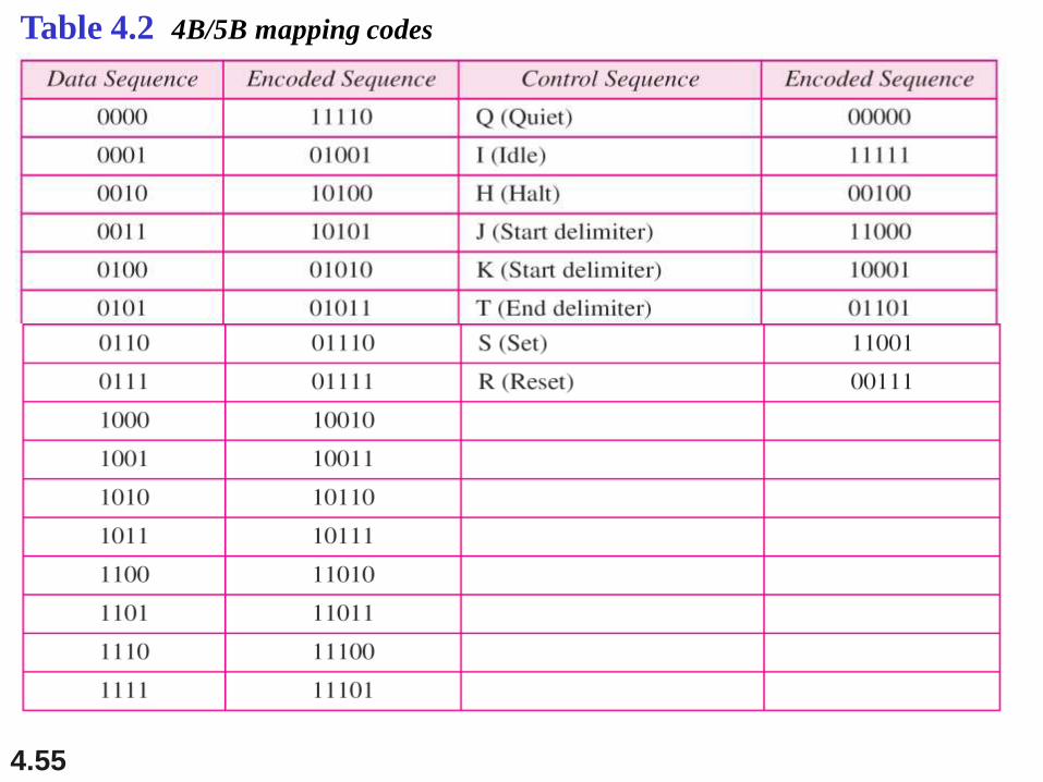
Table 4.2 4B/5B mapping codes
4.56
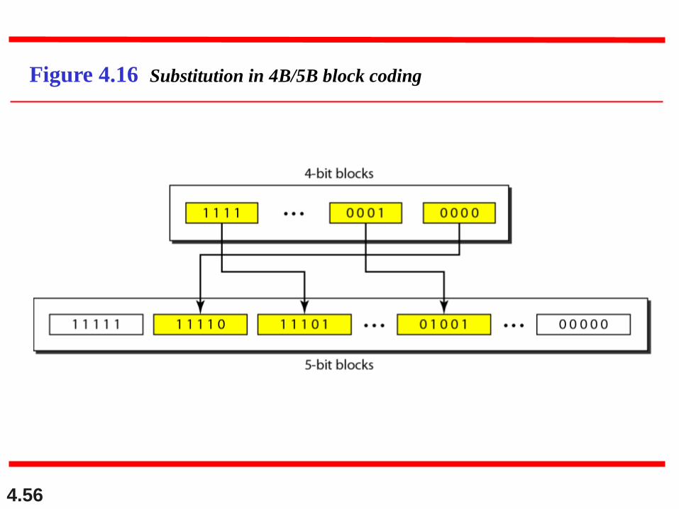
Figure 4.16 Substitution in 4B/5B block coding
4.57
Redundancy
A 4 bit data word can have 24 combinations.
A 5 bit word can have 25=32 combinations.
We therefore have 32 - 26 = 16 extra words.
Some of the extra words are used for control/signalling purposes.
4.58
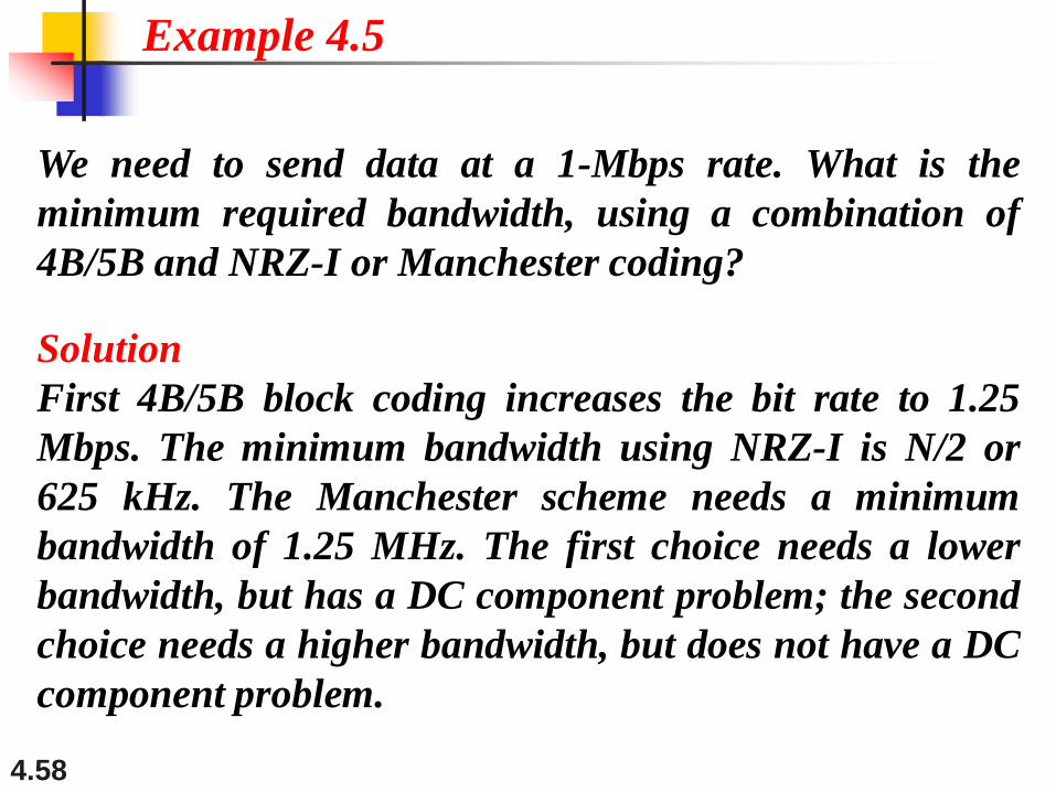
We need to send data at a 1-Mbps rate. What is the
minimum required bandwidth, using a combination of
4B/5B and NRZ-I or Manchester coding?
Solution
First 4B/5B block coding increases the bit rate to 1.25
Mbps. The minimum bandwidth using NRZ-I is N/2 or
625 kHz. The Manchester scheme needs a minimum
bandwidth of 1.25 MHz. The first choice needs a lower
bandwidth, but has a DC component problem; the second
choice needs a higher bandwidth, but does not have a DC
component problem.
Example 4.5
4.59
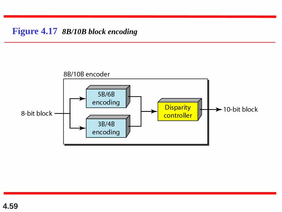
Figure 4.17 8B/10B block encoding
4.60
More bits - better error detection
The 8B10B block code adds more redundant bits and can thereby choose code words that would prevent a long run of a voltage level that would cause DC components.
4.61
Scrambling The best code is one that does not increase
the bandwidth for synchronization and has no DC components.
Scrambling is a technique used to create a sequence of bits that has the required c/c’s for transmission - self clocking, no low frequencies, no wide bandwidth.
It is implemented at the same time as encoding, the bit stream is created on the fly.
It replaces ‘unfriendly’ runs of bits with a violation code that is easy to recognize and removes the unfriendly c/c.
4.62
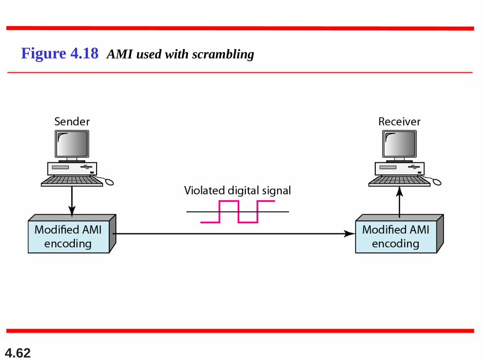
Figure 4.18 AMI used with scrambling
4.63
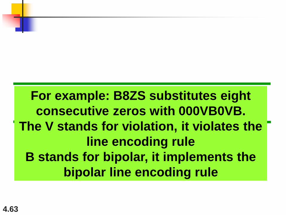
For example: B8ZS substitutes eight
consecutive zeros with 000VB0VB.
The V stands for violation, it violates the
line encoding rule
B stands for bipolar, it implements the
bipolar line encoding rule
4.64
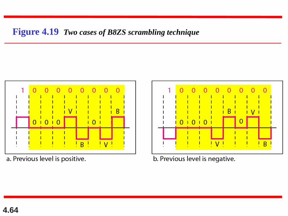
Figure 4.19 Two cases of B8ZS scrambling technique
4.65
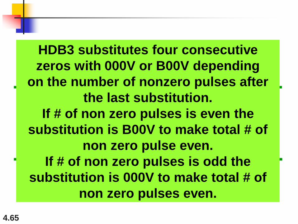
HDB3 substitutes four consecutive
zeros with 000V or B00V depending
on the number of nonzero pulses after
the last substitution.
If # of non zero pulses is even the
substitution is B00V to make total # of
non zero pulse even.
If # of non zero pulses is odd the
substitution is 000V to make total # of
non zero pulses even.
4.66
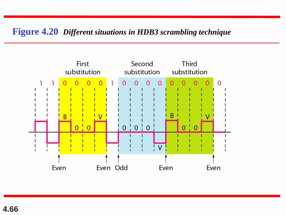
Figure 4.20 Different situations in HDB3 scrambling technique
4.1
4-2 ANALOG-TO-DIGITAL CONVERSION
A digital signal is superior to an analog signal because
it is more robust to noise and can easily be recovered,
corrected and amplified. For this reason, the tendency
today is to change an analog signal to digital data. In
this section we describe two techniques, pulse code
modulation and delta modulation.
Pulse Code Modulation (PCM)
Delta Modulation (DM)
Topics discussed in this section:
4.2
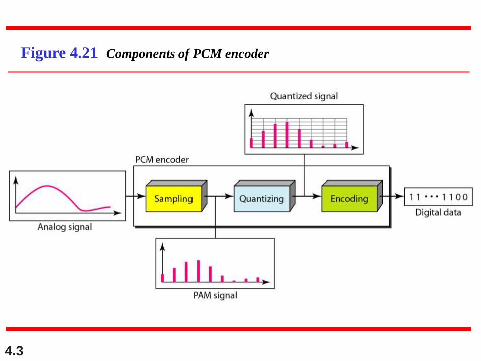
PCM PCM consists of three steps to digitize an
analog signal:1. Sampling
2. Quantization
3. Binary encoding
Before we sample, we have to filter the signal to limit the maximum frequency of the signal as it affects the sampling rate.
Filtering should ensure that we do not distort the signal, ie remove high frequency components that affect the signal shape.
4.3
Figure 4.21 Components of PCM encoder
4.4
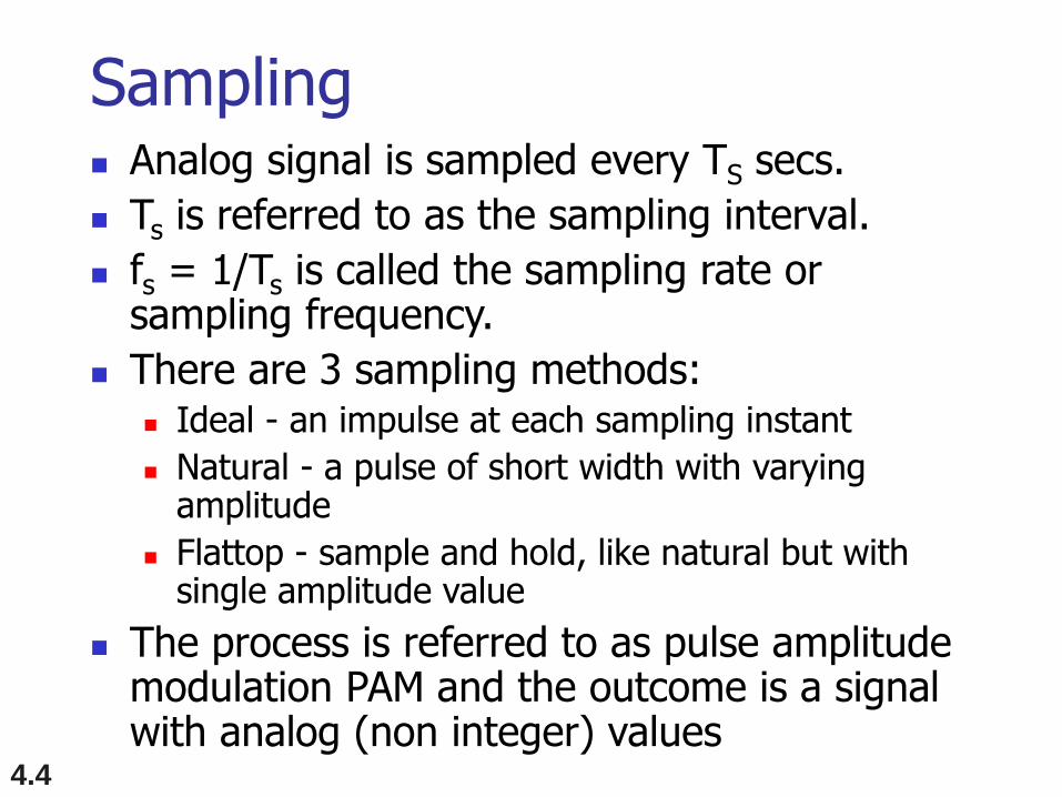
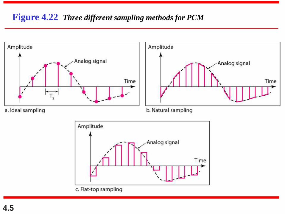
Sampling Analog signal is sampled every TS secs.
Ts is referred to as the sampling interval.
fs = 1/Ts is called the sampling rate or sampling frequency.
There are 3 sampling methods: Ideal - an impulse at each sampling instant
Natural - a pulse of short width with varying amplitude
Flattop - sample and hold, like natural but with single amplitude value
The process is referred to as pulse amplitude modulation PAM and the outcome is a signal with analog (non integer) values
4.5
Figure 4.22 Three different sampling methods for PCM
4.6
According to the Nyquist theorem, the
sampling rate must be
at least 2 times the highest frequency
contained in the signal.
Note
4.7
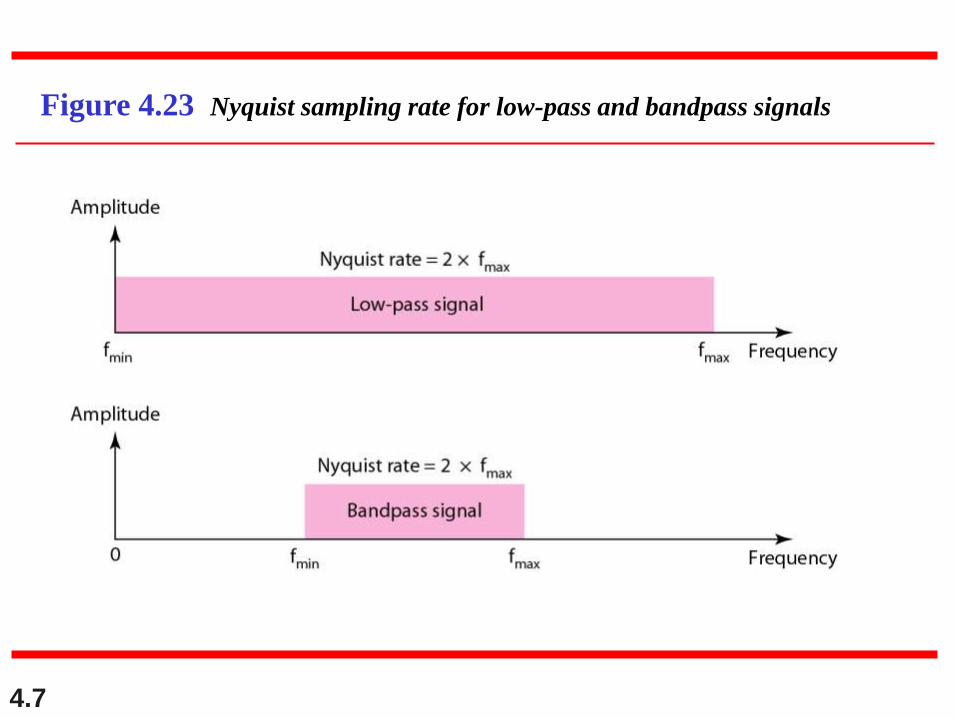
Figure 4.23 Nyquist sampling rate for low-pass and bandpass signals
4.8
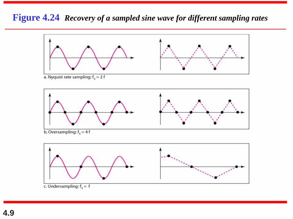
For an intuitive example of the Nyquist theorem, let us
sample a simple sine wave at three sampling rates: fs = 4f
(2 times the Nyquist rate), fs = 2f (Nyquist rate), and
fs = f (one-half the Nyquist rate). Figure 4.24 shows the
sampling and the subsequent recovery of the signal.
It can be seen that sampling at the Nyquist rate can create
a good approximation of the original sine wave (part a).
Oversampling in part b can also create the same
approximation, but it is redundant and unnecessary.
Sampling below the Nyquist rate (part c) does not produce
a signal that looks like the original sine wave.
Example 4.6
4.9
Figure 4.24 Recovery of a sampled sine wave for different sampling rates
4.10
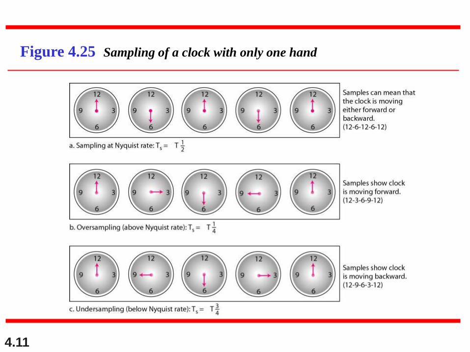
Consider the revolution of a hand of a clock. The second
hand of a clock has a period of 60 s. According to the
Nyquist theorem, we need to sample the hand every 30 s
(Ts = T or fs = 2f ). In Figure 4.25a, the sample points, in
order, are 12, 6, 12, 6, 12, and 6. The receiver of the
samples cannot tell if the clock is moving forward or
backward. In part b, we sample at double the Nyquist rate
(every 15 s). The sample points are 12, 3, 6, 9, and 12.
The clock is moving forward. In part c, we sample below
the Nyquist rate (Ts = T or fs = f ). The sample points are
12, 9, 6, 3, and 12. Although the clock is moving forward,
the receiver thinks that the clock is moving backward.
Example 4.7
4.11
Figure 4.25 Sampling of a clock with only one hand
4.12
An example related to Example 4.7 is the seemingly
backward rotation of the wheels of a forward-moving car
in a movie. This can be explained by under-sampling. A
movie is filmed at 24 frames per second. If a wheel is
rotating more than 12 times per second, the under-
sampling creates the impression of a backward rotation.
Example 4.8
4.13
Telephone companies digitize voice by assuming a
maximum frequency of 4000 Hz. The sampling rate
therefore is 8000 samples per second.
Example 4.9
4.14
A complex low-pass signal has a bandwidth of 200 kHz.
What is the minimum sampling rate for this signal?
Solution
The bandwidth of a low-pass signal is between 0 and f,
where f is the maximum frequency in the signal.
Therefore, we can sample this signal at 2 times the
highest frequency (200 kHz). The sampling rate is
therefore 400,000 samples per second.
Example 4.10
4.15
A complex bandpass signal has a bandwidth of 200 kHz.
What is the minimum sampling rate for this signal?
Solution
We cannot find the minimum sampling rate in this case
because we do not know where the bandwidth starts or
ends. We do not know the maximum frequency in the
signal.
Example 4.11
4.16
Quantization
Sampling results in a series of pulses of varying amplitude values ranging between two limits: a min and a max.
The amplitude values are infinite between the two limits.
We need to map the infinite amplitude values onto a finite set of known values.
This is achieved by dividing the distance between min and max into L zones, each ofheight
= (max - min)/L
4.17
Quantization Levels
The midpoint of each zone is assigned a value from 0 to L-1 (resulting in L values)
Each sample falling in a zone is then approximated to the value of the midpoint.
4.18
Quantization Zones
Assume we have a voltage signal with amplitutes Vmin=-20V and Vmax=+20V.
We want to use L=8 quantization levels.
Zone width = (20 - -20)/8 = 5
The 8 zones are: -20 to -15, -15 to -10, -10 to -5, -5 to 0, 0 to +5, +5 to +10, +10 to +15, +15 to +20
The midpoints are: -17.5, -12.5, -7.5, -2.5, 2.5, 7.5, 12.5, 17.5
4.19
Assigning Codes to Zones Each zone is then assigned a binary code.
The number of bits required to encode the zones, or the number of bits per sample as it is commonly referred to, is obtained as follows:
nb = log2 L
Given our example, nb = 3
The 8 zone (or level) codes are therefore: 000, 001, 010, 011, 100, 101, 110, and 111
Assigning codes to zones: 000 will refer to zone -20 to -15
001 to zone -15 to -10, etc.
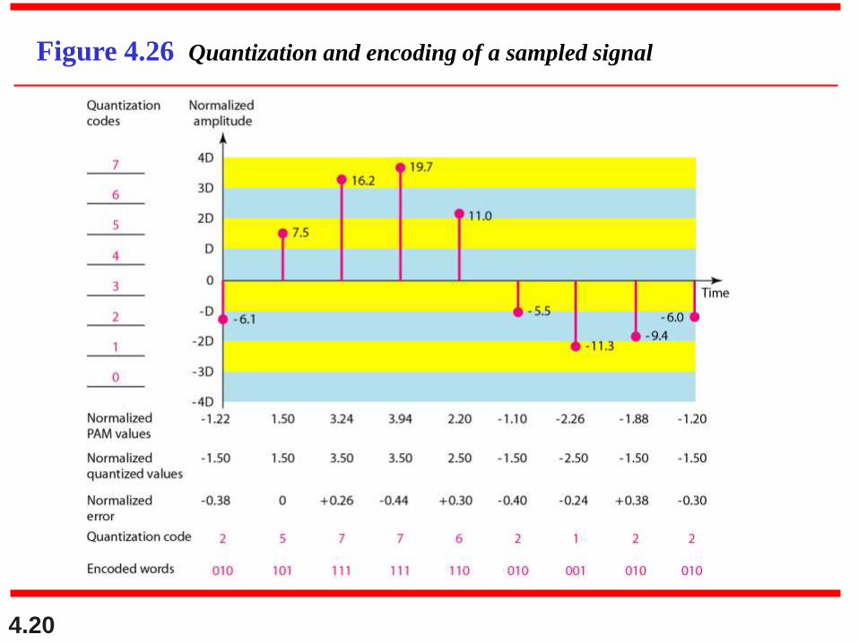
4.20
Figure 4.26 Quantization and encoding of a sampled signal
4.21
Quantization Error When a signal is quantized, we introduce an
error - the coded signal is an approximation of the actual amplitude value.
The difference between actual and coded value (midpoint) is referred to as the quantization error.
The more zones, the smaller which results in smaller errors.
BUT, the more zones the more bits required to encode the samples -> higher bit rate
4.22
Quantization Error and SNQR
Signals with lower amplitude values will suffer more from quantization error as the error range: /2, is fixed for all signal levels.
Non linear quantization is used to alleviate this problem. Goal is to keep SNQR fixed for all sample values.
Two approaches: The quantization levels follow a logarithmic curve.
Smaller ’s at lower amplitudes and larger’s at higher amplitudes.
Companding: The sample values are compressed at the sender into logarithmic zones, and then expanded at the receiver. The zones are fixed in height.
4.23
Bit rate and bandwidth requirements of PCM The bit rate of a PCM signal can be calculated form
the number of bits per sample x the sampling rate
Bit rate = nb x fs The bandwidth required to transmit this signal
depends on the type of line encoding used. Refer to previous section for discussion and formulas.
A digitized signal will always need more bandwidth than the original analog signal. Price we pay for robustness and other features of digital transmission.
4.24
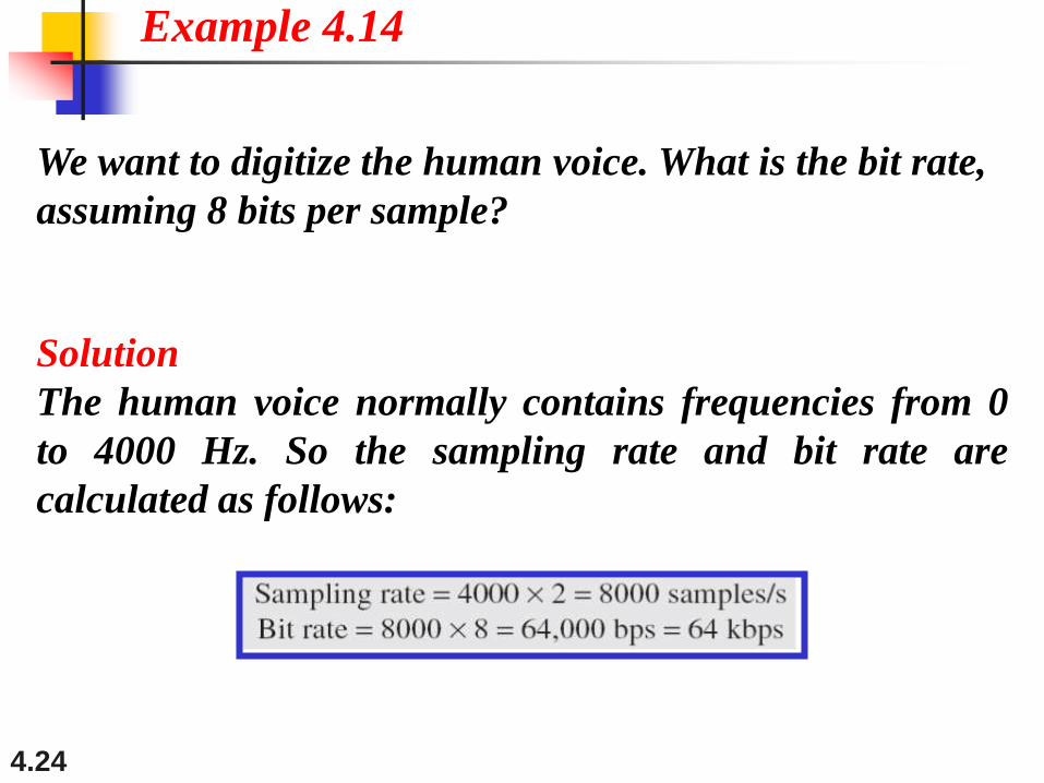
We want to digitize the human voice. What is the bit rate,
assuming 8 bits per sample?
Solution
The human voice normally contains frequencies from 0
to 4000 Hz. So the sampling rate and bit rate are
calculated as follows:
Example 4.14
4.25
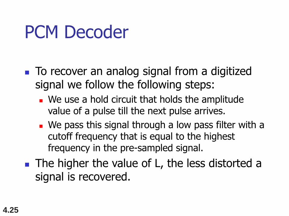
PCM Decoder
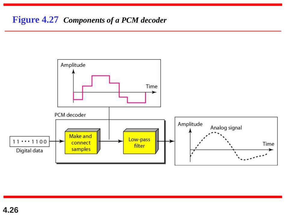
To recover an analog signal from a digitized signal we follow the following steps:
We use a hold circuit that holds the amplitude value of a pulse till the next pulse arrives.
We pass this signal through a low pass filter with a cutoff frequency that is equal to the highest frequency in the pre-sampled signal.
The higher the value of L, the less distorted a signal is recovered.
4.26
Figure 4.27 Components of a PCM decoder
4.27
We have a low-pass analog signal of 4 kHz. If we send the
analog signal, we need a channel with a minimum
bandwidth of 4 kHz. If we digitize the signal and send 8
bits per sample, we need a channel with a minimum
bandwidth of 8 × 4 kHz = 32 kHz.
Example 4.15
4.28
Delta Modulation This scheme sends only the difference
between pulses, if the pulse at time tn+1 is higher in amplitude value than the pulse at time tn, then a single bit, say a “1”, is used to indicate the positive value.
If the pulse is lower in value, resulting in a negative value, a “0” is used.
This scheme works well for small changes in signal values between samples.
If changes in amplitude are large, this will result in large errors.
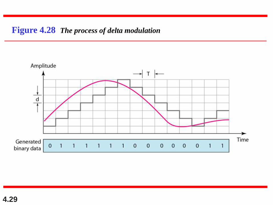
4.29
Figure 4.28 The process of delta modulation
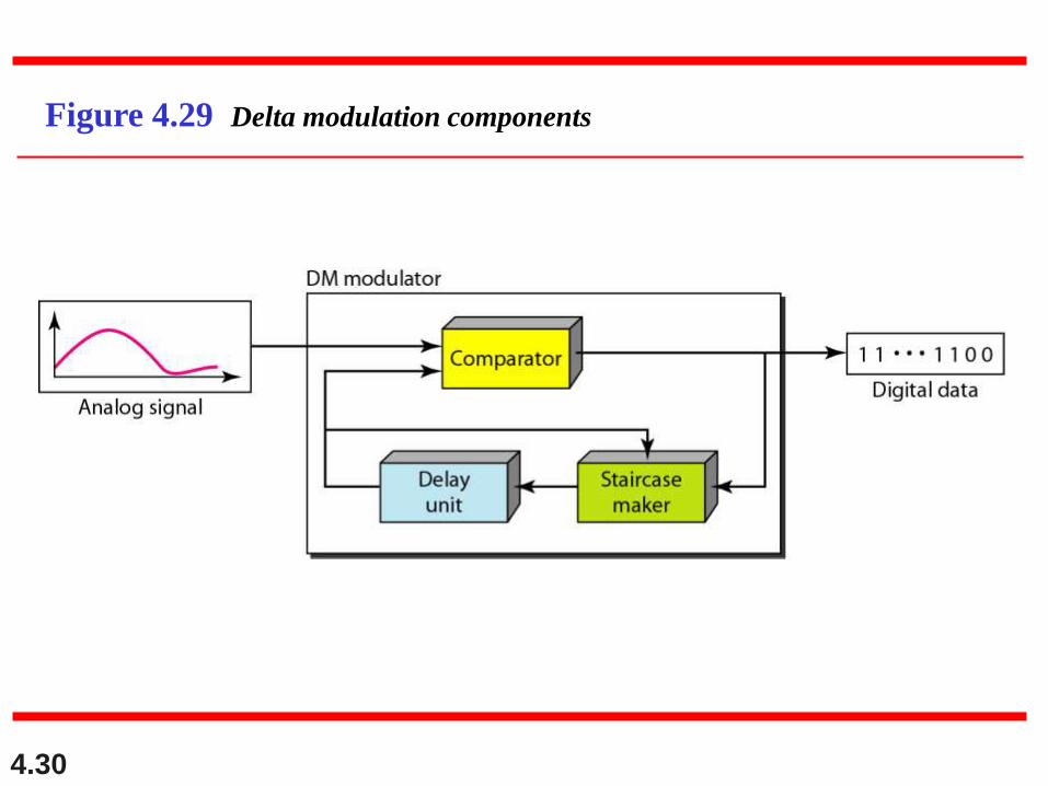
4.30
Figure 4.29 Delta modulation components
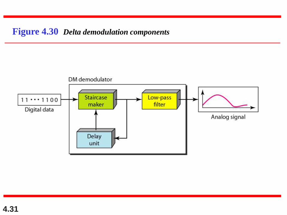
4.31
Figure 4.30 Delta demodulation components
4.32
Delta PCM (DPCM)
Instead of using one bit to indicate positive and negative differences, we can use more bits -> quantization of the difference.
Each bit code is used to represent the value of the difference.
The more bits the more levels -> the higher the accuracy.
4.33
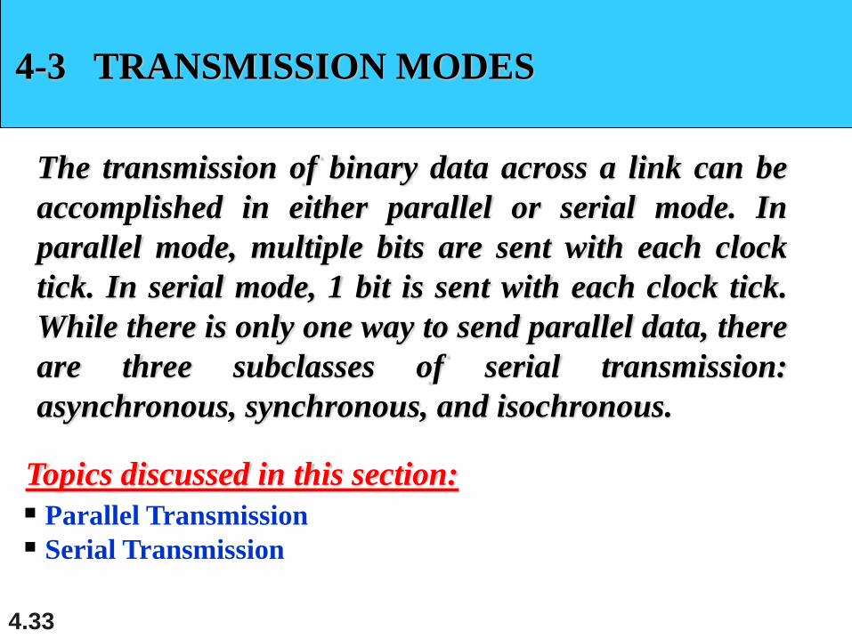
4-3 TRANSMISSION MODES
The transmission of binary data across a link can be
accomplished in either parallel or serial mode. In
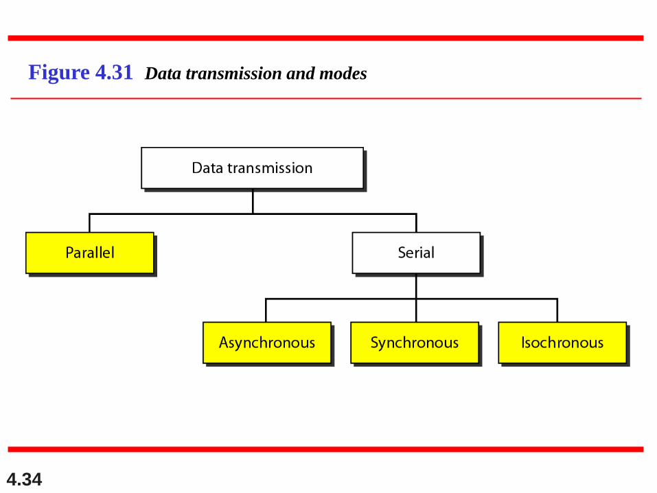
parallel mode, multiple bits are sent with each clock
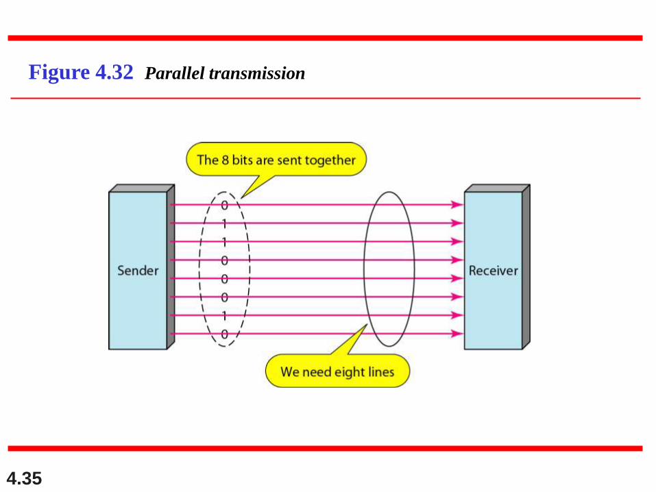
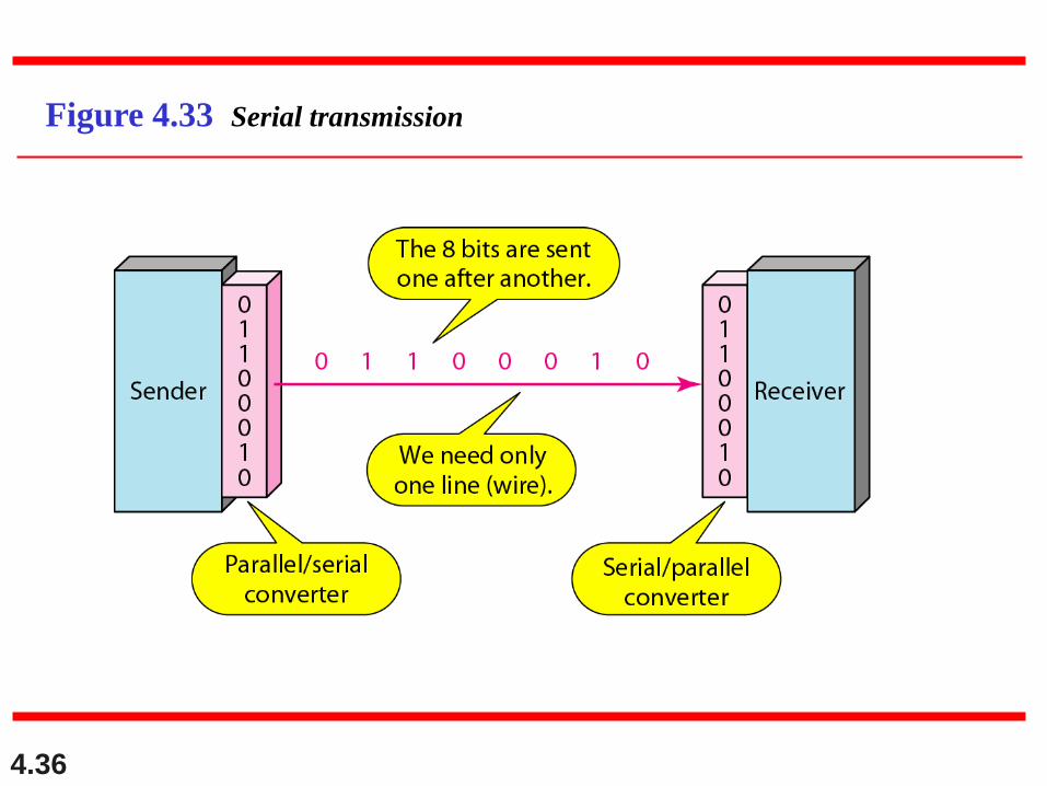
tick. In serial mode, 1 bit is sent with each clock tick.
While there is only one way to send parallel data, there
are three subclasses of serial transmission:
asynchronous, synchronous, and isochronous.
Parallel Transmission
Serial Transmission
Topics discussed in this section:
4.34
Figure 4.31 Data transmission and modes
4.35
Figure 4.32 Parallel transmission
4.36
Figure 4.33 Serial transmission
4.37
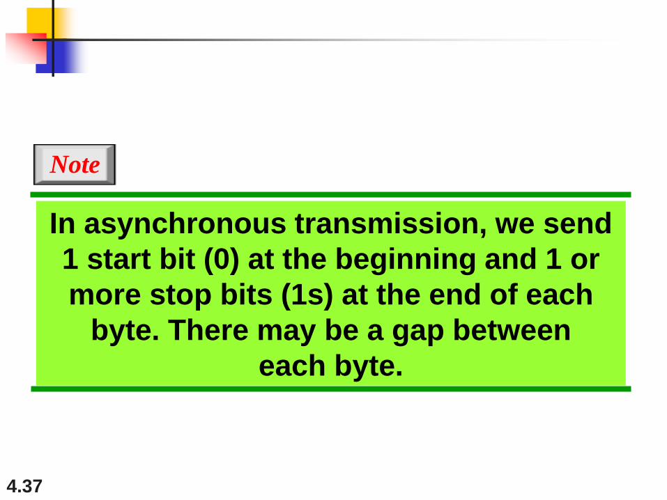
In asynchronous transmission, we send
1 start bit (0) at the beginning and 1 or
more stop bits (1s) at the end of each
byte. There may be a gap between
each byte.
Note
4.38
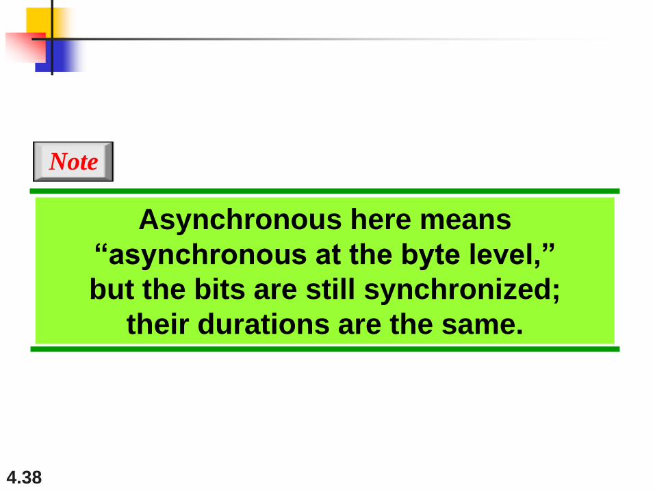
Asynchronous here means
“asynchronous at the byte level,”
but the bits are still synchronized;
their durations are the same.
Note
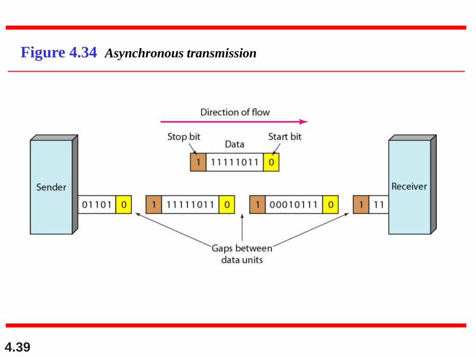
4.39
Figure 4.34 Asynchronous transmission
4.40
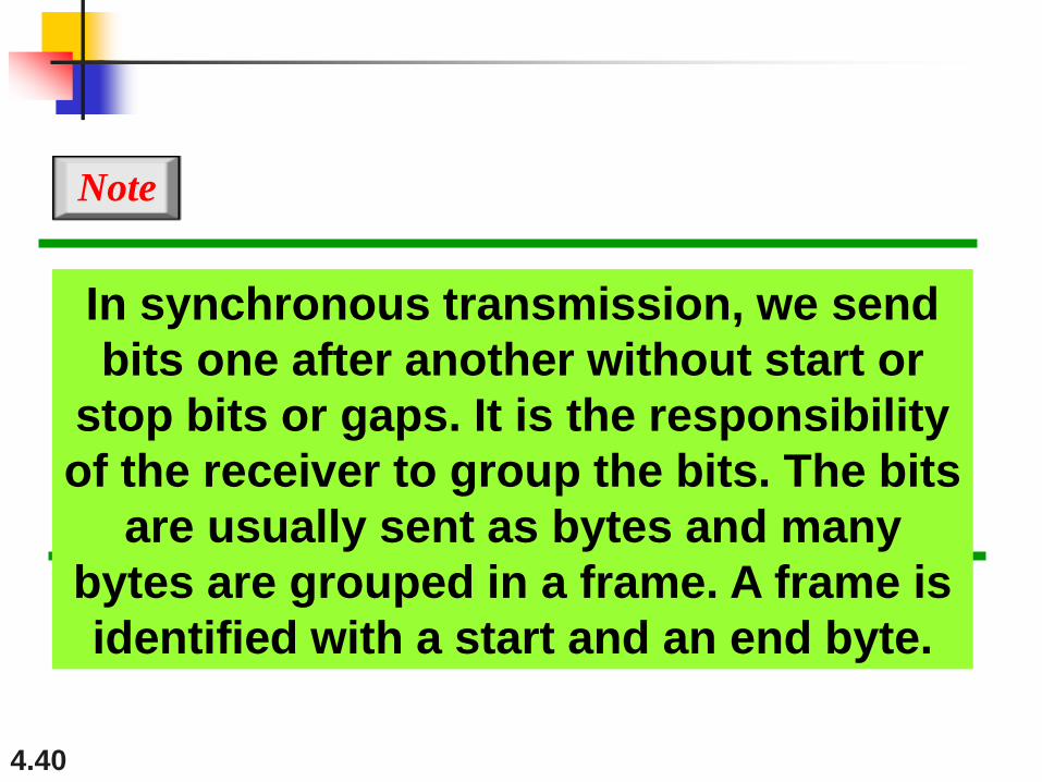
In synchronous transmission, we send
bits one after another without start or
stop bits or gaps. It is the responsibility
of the receiver to group the bits. The bits
are usually sent as bytes and many
bytes are grouped in a frame. A frame is
identified with a start and an end byte.
Note
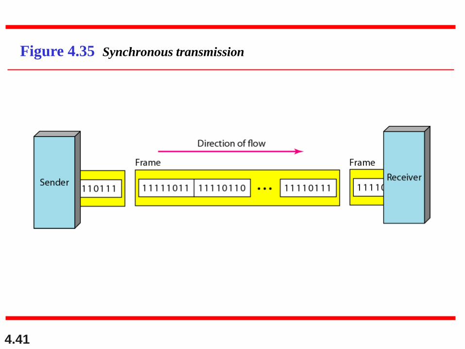
4.41
Figure 4.35 Synchronous transmission
4.42
Isochronous
In isochronous transmission we cannot have uneven gaps between frames.
Transmission of bits is fixed with equal gaps.
References
1. Computer Networks, A. S. Tenenbaum, D. J. Wetheral, Pearson India. 2. Data Communications and Networking, B.A. Forouzan, Tata McGraw Hill Education Private Limited. 3. Data and Computer Communications, William Stallings, Pearson-Prentice Hall.