Embed Size (px)
Citation preview

Chapter 4
Development of new Fractal features for the
Classification of Mammograms into
Normal, Benign and Malignant
Abnormalities in the mammograms include masses and microcalcifications, which
can be benign or malignant. Due to the presence of these abnormalities, the
regularity of the mammogram structure is altered, which changes its fractal
dimension. This chapter deals with the classification of mammograms based on
fractal dimension and features. To compute fractal dimension, three methods viz. the
Differential Box Counting Method, Blanket Method and Triangular Prism Surface
Area method were used. Since it was observed that fractal dimension cannot uniquely
distinguish between different classes of mammograms, six different fractal features
were derived from the above mentioned fractal dimension estimation methods. The
classification performances of these classifiers are evaluated using Receiver
Operating Characteristics (ROC).

56 Chapter 4. Development of New Fractal Features
4.1 Introduction
It is always desirable to develop computer-based methods to distinguish between
benign masses and malignant tumors while considering the traumatic nature and cost
of biopsy. Such methods can help in performing initial screening or second reading of
mammograms, and lend objective tools to help radiologists in analyzing difficult
cases and decide on biopsy recommendations.
The goal of this chapter is to develop an efficient new fractal feature derived
from fractal dimension, to assist radiologists’ in categorizing mammograms into
normal and abnormal.
Mandelbrot defined a number, associated with each fractal, called its fractal
dimension. It reflects the measure of complexity of a surface, the scaling properties of
the fractal i.e. how its structure changes when it is magnified. Thus fractal dimension
gives a measure of the irregularity of a structure.
Abnormal masses and microcalcifications such as benign and malignant are
used in this research. The fig 4.1 shows the different classes of mammograms.
Measures that can quantitatively represent shape, texture and complexity can assist in
the classification of mammograms into benign and malignant.
Fig 4.1 Different classes of mammograms
Mammograms
Normal Abnormal
Masses Microcalcifications
Benign Malignant Benign Malignant

56 Chapter 4. Development of New Fractal Features
Normal mammograms usually have a regular structure, but due to the presence of the
abnormal tissues the complexity of abnormal mammograms increases. Thus, naturally
they will have higher fractal dimension. Malignant tumors are generally rough and
have more irregularity whereas benign masses commonly have smooth, round, oval
contours.
Fig. 4.2 shows examples of mammograms from each class. In the normal
mammogram the ducts and tissues patterns are clearly visible. This makes the
interpretation of mammograms difficult, if microcalcifications or masses are
embedded in it.
Contd….
(b) Benign Mass
(a) Normal
4.1 Introduction 57

56 Chapter 4. Development of New Fractal Features
Fig.4.2 Different Classes of Mammograms: Original and ROI taken out from the mammogram
(a) Normal (b) Benign Mass (c) Malignant Mass (d) Benign Microcalcifications (e) Malignant
Microcalcifications
In this research, the property of fractional Dimension (FD) is used for the
classification of mammograms. Fractal dimension and different methods for the
computation of FD are discussed in the next section.
(c) Malignant Mass
(d) Benign Microcalcifications
(e) Malignant Microcalcifications
58 Chapter 4 Development of New Fractal features

56 Chapter 4. Development of New Fractal Features
4.2 Fractal Dimension
Mandelbrot in 1982 (Man 1982) has pioneered the use of fractals to describe objects
that possess self similarity at all scales and levels of magnification. Fractal objects
have irregular shapes and complex structures that cannot be represented adequately
by the traditional Euclidean dimension. Fractal Dimension (FD) is the fundamental
parameter for depicting fractal characteristics in fractal geometry. It is a number that
characterizes the ‘structure’ of the object. It assigns non integral dimension values to
objects that do not suit the traditional Euclidean space of objects.
For example, the dimension of a straight line is unity, but the dimension of a
jagged line is a fractional value falling between unity and two, depending on its
degree of jaggedness. The fractal dimension has been used in image classification to
measure surface roughness where different natural scenes such as mountains, clouds,
trees and deserts generate different fractal dimensions. The effective fractal
dimension estimation method is a precondition to utilizing fractal dimension to depict
fractal characteristic.
The parenchymal and ductal patterns in mammograms possess structures with
high local self-similarity which is the basic property of fractal objects (Li 1997).
Therefore, fractal method can be applied effectively for the analysis of mammograms.
It is observed that microcalcifications and masses are visible as objects which
appear to be added to the mammographic breast background. Some of them are
bright, some are faint. Compared with breast background tissue, they have less
structure. But the complexity increases in cancerous ones due to the presence of the
abnormal tissues. When abnormality in mammograms increases its complexity also
increases.
Next section covers the literature survey carried out on the current trends in
mammogram image processing and the use of fractals in the analysis of
mammograms.
4.2 Fractal Dimension 59

56 Chapter 4. Development of New Fractal Features
4.3 Literature Survey
There are large numbers of publications available in literature where fractals and
fractal based properties are applied for a wide range of applications as seen in chapter
3.
A system for identifying the boundary of liver in Computed Tomography
(CT) images was developed by Chen et. al. (Cen 1998) using fractal features and
deformable contour model. The normalized Fractional Brownian (NFB) motion
feature values, the correlation and sum entropy of the spatial gray-level dependence
matrices in conjunction with Modified Probability Neural Network (MPNN) were
used to discriminate between two types of liver tumors: hepotoma and hemageoma.
Pan and Lin (Pan 2010) classified the normal and cancerous liver tissues
using fractal dimension and Probabilistic Neural Network and obtained an accuracy
of 92.0% for the test set Wu et.al (Wu 1992) developed a new texture feature set
called multi-resolution fractal features based on the concepts of multiple resolution
imagery and fractional Brownian motion model. The performance of these features
was compared with the features like spatial gray-level dependence matrices, the
Fourier power spectrum, the gray-level difference statistics, and the Laws’ texture
energy measures. The new features were able to correctly classify three sets of
ultrasonic liver images - normal liver, hepatoma, and cirrhosis and 90% correct
classification was observed.
Local fractal dimensions of ECG signal were used by Raghav and Mishra
(Rag 2008) as a feature for the classification of ECG arrhythmia.
The fractal features extracted from fractal transformation (FT) by nonlinear
interpolation functions and Probabilistic Neural Network (PNN) has been introduced
by Lin et.al (Lin 2009) to recognize multiple cardiac arrhythmias.
Directional fractal dimension, which measures the degree of roughness along
a certain spatial direction along with the Multi-Layer Feed forward Neural Network
(MFNN), was used to perform classification of tissue section images of cells from
patients suffering from critical limb ischaemia by Shang et. al. (Sha 2000). The
classifier achieved a classification accuracy of 91%.
60 Chapter 4 Development of New Fractal features

56 Chapter 4. Development of New Fractal Features
The breast ultrasound images were first preprocessed to remove noise by
histogram equalization and morphological operations by Chang et. al. (Chg 2004) and
Chen et. al (Che 2005). The normalized factional Brownian motion feature vector
extracted from the processed images was used for classification with k means
classification method. The area under the ROC curve was found to be 0.9218.
A novel method of extraction of Region of Interest (ROI) in the breast
ultrasound (BUS) image for the fully automatic classification was shown by Liu et.al
(Liu 2010). The Area Under the Curve (AUC) of the generated ROIs was obtained as
0.968.
Potlapalli (Pot 1998) developed a new Incremental Fractional Brownian
Motion (IFBM) for the classification of textures.
High dimensional biologically inspired feature (BIF) and its variations have
been demonstrated by Song and Tao (Son 2010) to be effective and efficient for scene
classification.
A new adaptive fuzzy classification algorithm, called influential rule search
scheme (IRSS), was developed by Chatterjee and Rakshit (Cht 2004) for automatic
construction of the fuzzy membership functions (MFs) and the fuzzy rule base from
an input-output data set.
A novel pattern recognition approach was proposed by Baskes et.al
(Bac2010) based on the Complex Network Theory and complexity analysis. It was
illustrated how a shape contour can be effectively represented and characterized as a
complex network in a dynamic evolution context, and how degree based
measurements can be used to estimate the network complexity through Multi-Scale
Fractal Dimension.
For automatic target recognition (ATR) using radar, the local fractal
dimensions of a synthetic aperture radar image have been used as features to classify
ground targets by Mishra et. al (Mis 2007).
The concept of lacunarity and the use of two lacunarity estimation methods
(i.e., binary, gray scale) in texture analysis and classification of high resolution urban
images were discussed by Myint and Lam (Myi 2005). When compared with the
4.3 Literature Survey 61

56 Chapter 4. Development of New Fractal Features
traditional spectral based classification approach with an accuracy of 55%, lacunarity
approaches improved the accuracy dramatically to 92%.
Hadjileontiadis (Had 2009) presented an automatic classification method to
discriminate the types of discontinuous breath sounds (DBSs), i.e., fine crackles
(FCs), coarse crackles (CC), and squawks (SQ), using lacunarity. They have shown
that it provided an efficient discrimination among DBS with a mean classification
accuracy of 100%, 99.62%–100%, and 99.75%–100% for the comparison groups of
{FC-CC, FC-SQ}, {CC-SQ}, and {FC-CC-SQ}, respectively
A comparative analysis of different feature extraction methods for fingerprint
classification based on orientation maps (OMs) and Gabor filters was presented by
Rajanna et.al (Raj 2009).
The selection of useful features is a fundamental problem in any
classification task. Irrelevant and redundant features degrade classification
performance. Therefore, Levi and Ullman (Lev 2010) dealt with the goal of selecting
a set of features, which is optimum for classification and have minimum redundancy.
Samarabandu et. al. (Smb 1993) used the concepts of mathematical
morphology to compute the fractal dimension of bone x-rays. This gives an additional
advantage of encoding structural information via the selection of a structuring
element and also gives a robust texture measure of trabecular bone structures.
Lin et. al. (LiK 2001) computed fractal dimension using differential box
counting method for extracting eye pairs which achieves an overall hit rate of 100%
without head tilt.
It was found by Jiang et. al. (Jng 2009) that, the contour fractal dimension as
well as the contour and nervure fractal dimension can be used to distinguish between
leaves of different types of plants effectively.
The correlation fractal dimension was used by Langi and Kinsner (Lan 1995)
as a distinguishing feature for characterizing consonant phonemes that improved the
speech recognition performance.
Kinsner and Vera (Kin 2006) classified real world self affine non stationary
signals from non linear systems, by the computation of the Variance of the Fractal
Dimension Trajectory (VFDT). The features extracted from VFDT were applied to
62 Chapter 4 Development of New Fractal features

56 Chapter 4. Development of New Fractal Features
complex domain neural network and probabilistic neural network gave a
classification accuracy of 87%.
A new method for finding the fractal dimension which is less sensitive to
sampling frequency was developed by Senevirathne et.al. (Sen 1992)
Fractal dimension was used by Fekkai et. al. (Fek 2000) to characterize the
fluctuations in speech signal and was utilized for the recognition of isolated speech.
The degree of correlation between breast parenchymal patterns was assessed
using a simple fractal dimension method by Caldwell et. al (Cal 1990). Velanovich
(Vel 1998) quantified complex shapes in mammograms by fractal analysis and using
this they were classified into benign and malignant with 100% sensitivity and 63%
specificity.
The lesions in the mammograms were extracted by SzCkely and Pataki (SzC
2003) by first binarizing the image and then using the shape descriptors derived from
moment based and PCA based methods.
Kobatake et.al (Kob 1994) enhanced cancerous tumors by the newly
developed adaptive iris filter. Shape analysis was then applied to discriminate
between malignant tumors and others. For them the average number of false positives
per image was only 0.18 while the true positive detection rate was 100%.
Brake and Karssemeijer (Bra 1999) developed three different pixel-based
methods for detecting masses based on scale. Their first method utilizes convolution
of a mammogram with the Laplacian of a Gaussian, the second method was based on
correlation with a model of a mass, and the third was a new one, based on statistical
analysis of gradient-orientation maps.
Curvelet transform was applied to classify different types of mammograms
by Eltoukhy (Elt 2009). Baeg and Kehtarnavaz (Bae 2002) introduced an automatic
CAD system for the classification of mammogram masses into benign and malignant.
Here, the two features namely, denseness and architectural distortion were fed to the
neural network classifier, which gave an area under the curve of 0.90 in the ROC
analysis.
4.3 Literature Survey 63

56 Chapter 4. Development of New Fractal Features
Faye et. al (Fay 2009) decomposed mammograms using wavelets to extract a
set of coefficients to differentiate between normal and abnormal and then to classify
the type of abnormality as benign or malignant tumor.
An appropriate Gabor filter is chosen which can identify the texture
differences between normal and abnormal mammograms. To increase classification
efficiency and reduce the feature space, statistic t-test and its p- values for feature
selection and weighting were proposed by Don and Wang (Don 2009).
Rangayyan et. al. (Ran 1997) investigated the use of a new measure of edge
strength or acutance of the tumor ROI, to characterize the fuzzy nature of malignant
tumor boundaries and the sharply defined nature of benign masses. Acutance alone
gave a benign/malignant decision accuracy of about 95% with the MIAS database.
They also analyzed the effectiveness of shape factors like compactness, in
distinguishing between circumscribed and spiculated tumors, achieving an accuracy
of 92.3%.
Khuwaja and Rezq (Khu 2004) proposed a bi-modal artificial neural network
(ANN) for breast cancer classification system. The microcalcifications are extracted
with adaptive learning vector quantization networks that are trained with
cancer/malignant and normal/benign breast digital mammograms. The performance
of the networks is evaluated using ROC curve analysis which gave a sensitivity-
specificity of 98.0-100.0 for the CC view and 96.0-100.0 for the MLO view.
Since fractals possess properties, it can be easily approximated to
physiological entities. Therefore to have a better classification accuracy fractal
dimension and fractal based features are used in this research.
The three fractal dimension estimation methods present in literature are
discussed in the next section.
4.4 Fractal Dimension Estimation Methods
In this research, three methods for computing fractal dimension were considered.
They are the Differential Box Counting, Blanket and Triangular Prism Surface Area
methods. The discussion starts with the conventional box counting method.
64 Chapter 4 Development of New Fractal features

56 Chapter 4. Development of New Fractal Features
4.4.1. Box Counting Method
The simplest method to compute fractal dimension is the box counting
method, which is based on the concept of self-similarity. In a Euclidean n-space, a
bounded set A , is said to be self-similar when A is the union of rN distinct (non
overlapping) copies of itself, each of which has been scaled down by a ratio of r . The
fractal dimension D is related to the number rN and the ratio r as follows:
( )( )r
ND r
r 1log
loglim
0→
= (4.1)
where rN is the minimum number of distinct fractal copies of A in the scale r i.e.
the number of boxes of size r . The union of rN of all the distinct copies must cover
the entire set A completely.
The main difficulty with this method is that real world images are seldom self
similar. Also, this method is appropriate for finding the fractal dimension of binary
images only. Hence, the box counting method was modified and made suitable to be
applied to gray level images.
4.4.2 Differential Box Counting Method
Sarkar and Chaudhuri (Sar 1994) proposed the differential box counting
(DBC) method by modifying the box counting method and have compared it with
other conventional methods. Consider an image of size MM × pixels. Assume that
the image is represented in a 3D space, with ( )yx, axes denoting the spatial co-
ordinates, while the z axis denoting the gray level. The fig.4.3 shows the image plane
and the image intensity surface for estimating the fractal dimension using the
differential box counting method.
The ( )yx, space is partitioned into grids of size ss × , where 12 >≥ sM , is
an integer. Then, Msr = .On each grid there is a column of boxes of size 'sss ×× ,
where 's is the side along the z direction corresponding to the gray level axis. If the
total number of gray levels is G , then, sMsG =' . Numbers from ,...2,1 are
4.4 Fractal Dimension Estimation Methods 65

56 Chapter 4. Development of New Fractal Features
assigned to the boxes starting from the lowest gray level value. Let the minimum and
the maximum gray level of the image in the ( )thji, grid fall in box number k and l ,
respectively.
Fig 4.3 Schematic for finding the FD using Differential Box counting method
The contribution of rN in ( )thji, grid is given by:
( ) 1, +−= kljinr (4.2)
Due to the differential nature in computing rn this method is called differential box
counting method. The contributions from all grids are found by:
( )∑=ji
rr jinN,
, (4.3)
rN is computed for different values of s i.e. different values of r . Using equation
(4.2) D , the fractal dimension can be estimated, from the least square linear fit of
( )rNlog against ( )r1log . A random placement of boxes is applied in order to reduce
quantization effects.
66 Chapter 4 Development of New Fractal features

56 Chapter 4. Development of New Fractal Features
4.4.3 Blanket Method
Peleg et al (Pel 1984) used the blanket method approach of measuring the
fractal dimension. Image can be viewed as a hilly terrain surface whose height from
the normal ground is proportional to the image gray value as shown in fig. 4.4.
A small portion of mammogram is taken out. The z axis gives the gray level.
Gray levels of this region vary from 185 to 230. The upper gray levels are denoted by
red color while the lower gray levels are given blue color. Then all points in the three
dimensional space at distance ε from the surface on both sides create a blanket of
thickness ε2 .
Fig 4.4 Gray Level of Mammogram
The estimated surface area is the volume occupied by the blanket divided
by ε2 . All points in the three dimensional space at distance ε from the surface are
considered, covering the surface with a "blanket" of thickness ε2 . The covering
blanket is defined by its upper surface εu and lower surface εb .
Initially, i.e. when 0=ε , the upper and lower surfaces are given by the same
gray level function ( )jig , , i.e.
Upper
surface εu
Lower
surface εb
4.4 Fractal Dimension Estimation Methods 67

56 Chapter 4. Development of New Fractal Features
( ) ( ) ( )jigjibjiu ,,, 00 == (4.4)
For ,...2,1=ε the blanket surfaces are defined as:
( ) ( )( ) ( )
( )
+= −≤−
− nmujiujiujinm
,max,1,max, 11,,
1 εεε (4.5)
( ) ( )( ) ( )
( )
−= −≤−
− nmbjibjibjinm
,min,1,min, 11,,
1 εεε (4.6)
A point ( )fyx ,, will be included in the blanket of ε when ( ) ( )yxufyxb ,, εε ≤< .
The blanket definition uses the fact that the blanket of the surface for radius ε
includes all the points of the blanket for radius 1−ε , together with all the points within
radius 1 from the surfaces of that blanket. Expressions (4.5) and (4.6) ensure that the
new upper surface and lower surfaces are higher/lower by at least 1 from 11 −− εε bu ,
and also at distance at least 1 from 11 −− εε bu in the horizontal and vertical directions.
The volume of the blanket is computed from εu and εb by the following equation:
( ) ( )( )∑ −=ji
jibjiuV,
,, εεε (4.7)
The surface area of the blanket can be measured from the volume as:
21−−
= εεε
VVA (4.8)
Another definition for the surface area is εε 2V . This is necessary, since
εV depends on all small scales features. Subtracting 1−εV isolates just those features
that change from scale 1−ε to scaleε . When a pure fractal object is analyzed, both
definitions are identical since property changes are independent on scale, and
measurements between any two different scales will yield the same fractal dimension.
However, for non fractal objects, this isolation from the effects of smaller scale
features is necessary. The definition in the above equation (4.8) gives reasonable
measures for both fractal and non fractal surfaces.
According to Mandelbrot (Man 1982), the area of the fractal surface is:
68 Chapter 4 Development of New Fractal features

56 Chapter 4. Development of New Fractal Features
,...2,1,2 =≈ − εεεD
FA (4.9)
where D is the fractal dimension. When plotting εA versus ε on a log-log scale, a
straight line is obtained with slope 2 - FD. This curve is not a straight line for non
fractal surfaces. The slope of the best fitting straight line gives the fractal signature
S(ε) (discussed in detail in section 4.4.3.1). For fractal objects S(ε) should be equal to
2-D for all ε.
i.e. Fractal Signature S(ε) or Slope FD−= 2 (4.10)
According to Tao et. al (Tao 2000) the fractal dimension can be computed from
equation (4.9) as follows. A line can be drawn when any two points are known.
Therefore, two values ε and 1−ε are used for the computation of fractal dimension
as:
DFA
−≈ 211
εε , DFA
−≈ 222
εε
or, D
D
A
A
−
−
≈22
21
2
1
ε
ε
ε
ε
Taking logarithm on both sides:
( ) ( )( ) ( )2212
22
loglog
loglog2 21
εε
εε
−
−≈−
AAD
( ) ( )( ) ( )2212
22
loglog
loglog2 21
εε
εε
−
−−≈
AAD (4.11)
4.4.3.1 Fractal Signature
The magnitude of the fractal signature S (ε), is related to the amount of detail included
on the blanket of size ε. High value of the signature S (ε), is associated with large gray
level variations at distance ε. High value of S (ε) at small ε is due to high frequency
gray level variations while high values for larger ε result from major low frequency
variations. Thus the fractal signature S (ε) gives important information about the
fineness of the variation of the gray level surface.
4.4 Fractal Dimension Estimation Methods 69

56 Chapter 4. Development of New Fractal Features
The different types of mammograms are compared based on differences between
their fractal signatures. The distance for two different images with signatures Si (ε) and
Sj(ε) is defined by:
( ) ( )
−
+−= ∑
2
12
1
log)(S)(Sj,iD2
ji
ε
εεε
ε
(4.12)
The weighting factor of ( ) ( )[ ]5.05.0log −ε+ε is due to the unequal spacing of the
points in the log-log scale.
4.4.3.2 Differential Fractal Signatures and Distance Measurement
Consider an image of light particles scattered over a dark background. Since the
high gray level value stands for white, the expression for minimum in equation (4.6)
will shrink the light regions, and the rate of this shrinking will only depend on the
shape property of the particles. The maximum operator in equation (4.5) however will
shrink the background regions and the rate of this shrinking will mainly be affected by
the distribution of particles. To consider this asymmetry, the surface area measurement
is divided into two parts: measuring the area of the gray level surface when viewing
from “above “and measuring the area when viewing the surface from “below”. Thus,
the definition of volume in equation (4.7) can be changed to the following two
definitions of “upper volume” V+ and “lower volume” V- as follows:
( ) ( )∑ −= ε+ε
j,i
j,igj,iuV (4.13a)
and
( ) ( )∑ ε−ε −=
j,i
j,ibj,igV (4.13b)
Similarly the expression for area in (4.8) is also changed into “top area” A+ and
“bottom area” A- as follows:
2
VVA 1
−−ε
+ε+
ε
−= (4.14a)
and
2
VVA 1
−−ε
−ε−
ε
−= (4.14b)
70 Chapter 4 Development of New Fractal features

56 Chapter 4. Development of New Fractal Features
The two different fractal signatures S+ and S- are computed as before. The S- plot
represents the shape of the parts while the S+ graphs represent the background of the
image.
Analyzing again, now by differentiating between the top and bottom areas, the
differential distance D’ between two textures i and j are defined as:
( ) ( ) ( )( ) ( ) ( )( )∑
−
+
−+−= −−++
ε ε
εεεεε
2
12
1
log.SSSSj,iD2
ji
2
ji'
(4.15)
4.4.4 Triangular Prism Surface Area Method
The third method to measure fractal dimension used in this research work is the
Triangular Prism Surface Area (TPSA) method proposed by Clarke (Cla 1986).The
schematic representation for the measurement of the triangular prism surface area is
shown in fig. 4.5.
The original image is assumed to be of size MM × as in the above method.
The steps required for finding fractal dimension using TPSA method, discussed by
Tang and Wang (TaM 2005) are given below:
Step 1: The image is divided into different grids of size r. Let the four points of
every square grid correspond to four points A , B , C , D on the fractal surface.
These points are represented by the gray level value at that point. i.e. height
of this grid corresponds to the gray level values ( )jih , , ( )1, +jih , ( )jih ,1+
and ( )1,1 ++ jih respectively.
Step 2: The distance from the ground to the center of each grid cell of the four
heights of the adjacent points can be calculated as:
( ) ( ) ( ) ( )[ ]1,1,11,,4
10 +++++++= jihjihjihjihh (4.16)
4.4 Fractal Dimension Estimation Methods 71

56 Chapter 4. Development of New Fractal Features
Fig. 4.5 Schematic for finding TPSA
Step 3: The top of the grid is divided into four triangles ABE , ACE , CDE and BDE .
The area of the triangle ABE is determined as:
( )( )( )1111111 clblallS ABE −−−= (4.17)
where ( )11112
1cbal ++= (4.18)
( ) ( )[ ] 22
1 r1j,ihj,iha ++−= (4.19a)
( )[ ] 22
01 r5.0hj,ihb +−= (4.19b)
( )[ ] 22
01 r5.0h1j,ihc +−+= (4.19c)
Step 4: The area of the remaining triangles ACE , CDE and BDE are also found out
similarly. Thus, the approximate real area of a fractal surface in a given grid
cell with a scale of rr × is given by:
( ) BDECDEACEABE SSSSjiS +++=, (4.20)
Step 5: Considering the entire image, the total area of the fractal surface is:
72 Chapter 4. Development of New Fractal features

56 Chapter 4. Development of New Fractal Features
( ) ( )( )
∑=
=rN
1j,i
j,iSrS (4.21)
where ( )rN is the total number of the regular squares of size rr × .
Step 6: In fractal geometry, the total area of the fractal surface ( )jiS , , the scale δ
and the fractal dimension D are related by
( ) D2r~rs
− (4.22)
Repeat steps 1-5 with different values of r . Then ( )( )rSlog and ( )rlog is plotted in
the loglog− co-ordinate system. If the slope of the best fitting straight line joining
these points is b , the fractal dimension D of the image is:
bD −= 2 (4.23)
4.5 Fractal Features
The main problem with the fractal dimension approach is that it cannot uniquely
characterize the texture pattern. Different textures may have the same fractal
dimension. This is due to the combined differences in coarseness and directionality i.e.
dominant orientation and degree of anisotropy (Man 1982). Hence features based on
fractal dimension were considered. Five features based on fractal dimension used in
texture segmentation (Chd 1995) were tried for characterizing mammograms. They are
the FD of the original image, the high gray valued image, the low gray valued image,
the horizontally smoothed image and vertically smoothed image. In addition to these
features a new fractal feature was derived from the average of four pixels of the image.
The different fractal features utilized in this research are discussed below.
4.5.1 Fractal Feature 1 (f1)
The FD of the original image I1 is computed using overlapping windows of
size ( ) ( )1212 +×+ WW . Thus, at point ( )ji, the first feature value ( )jiF ,1 is defined as
( ) ( ){ }WkWkjliIFDjiF ≤≤−++= ,;,, 11 (4.24)
4.5 Fractal Features 73

56 Chapter 4. Development of New Fractal Features
where, FD is the fractal dimension computed using any of the methods described in
section 4.4. Since the fractal dimension is greater than the topological dimension, the
value of 1F is between 2 and 3. The normalized feature is defined as ( ) 2,11 −= jiFf ,
such that 10 1 ≤≤ f .Thus all the normalized fractal features are between 0 and 1.
4.5.2. Fractal Features 2 and 3 (f2 and f3)
The two modified images called high and low gray-valued images, 2I and 3I
respectively are defined as:
( )( ) ( )
>−
=otherwise
LjiIifLjiIjiI
0
,,,, 1111
2 (4.25)
( )( ) ( )
( ) −>−
=otherwisejiI
LjiIifLjiI
,
255,,255,
1
212
3 (4.26)
where
2min1 avgL += ; (4.27a)
2max2 avgL −= ; (4.27b)
with maxg , ming and av denoting the maximum, minimum and average gray value
in the original image 1I , respectively. Even if two images 1I and 1J have the same
fractal dimension, their high gray-valued images 2I and 2J may not have an
identical roughness and so their FDs would be different. The same holds for 3I and
3J . The normalized fractal features 2f and 3f are computed from 2I and 3I
similar to the computation of 1f from 1I .
4.5.3 Fractal Feature 4 and 5 (f4 and f5)
Fractal dimension of an image is directly related to its roughness and therefore its
value will be reduced by gray level smoothing. If the texture is smoothed along the
direction of its dominant orientation, the FD will be affected least for a highly oriented
74 Chapter 4 Development of New Fractal features

56 Chapter 4. Development of New Fractal Features
texture. But when the smoothing direction is perpendicular, the FD will be
considerably reduced. A texture having a low degree of anisotropy will show an
identical effect on the FD, irrespective of the smoothing direction.
Images can be smoothed in the horizontal and vertical direction as:
( ) ∑−=
++
=W
Wk
kjiIW
jiI ),(12
1,4
(4.28)
( ) ∑−=
++
=W
Wk
jkiIW
jiI ),(12
1,5
(4.29)
W is the same as in fractal feature 1f . The normalized FD features 4f and 5f are
computed similar to that of 1f .
4.5.4 Fractal Feature 6 (f6)
A new fractal feature is derived from the smoothened image obtained by computing
the average of four neighboring pixels using a non overlapping 4×4 window. The new
image is given by:
( ) ( )∑ ∑= =
=2
1
2
16 ,
4
1,
i j
jiIjiI (4.30)
Here, four pixels in the image were replaced with a single pixel. Thus the size of the
image will be reduced by 4 (i.e. MM × image is reduced to 22 MM × ). This
reduces the difference between the minimum and maximum gray levels in the new
image. This in turn, reduces the variance of the gray levels in the prism (in fig. 4.5).
So when the area of the triangles formed from the prism is calculated, in the TPSA
method, which is used for evaluating6f , the area will be reduced. This means that the
spread of the area, which is used to calculate, 6f will be reduced while considering
regions of mammogram containing normal and cancerous tissues. Thus, when the
feature 6f is calculated, the overlap between the values for the different categories
can be avoided. This overlapping of feature values among the different categories was
the problem with all the fractal features from 1f to
5f . Feature 6f is novel and features
1f to5f are used for the comparison of classification result. A good feature should
remain unchanged with changes within the class and should reveal important
4.5 Fractal Features 75

56 Chapter 4. Development of New Fractal Features
differences when discriminating between patterns of different classes (Bas 2004) and
this is satified by the results obtained with f6.
4.6 Conventional features used for the comparison with
fractal features
The performance of the fractal features in discriminating the different classes of
mammograms was compared with the following conventional features based on
intensity, texture, etc.
4.6.1 Statistical Descriptors
a. Mean: The mean of a random variable is defined using the probability
density or mass function. It provides a measure of central tendency of the
distribution. (Mtz 2008)
∑=
=N
k
kk
n
nf
1
µ (4.31)
where N denotes the gray levels of the mammogram, kf is the kth gray level
and kn is the number of pixels having gray level kf and n is the total number
of pixels in the region considered (Min 2003a)
b. Variance: The variance of a random variable is a measure of the dispersion
in the distribution. If the random variable has a large variance, then the
observed value of the random variable is more likely to be far from the
mean µ . The square root of variance is called standard deviation (Mtz 2008).
( )∑
=
−=
N
k
kk
n
nf
1
22 µ
σ (4.32)
c. Skewness: It is a measure of the asymmetry of the data around the sample. If
the skewness is negative, the data is spread out more to the left of the mean
than to the right. If skewness is positive, the data are spread out more to the
right. The skewness of the normal distribution or any perfectly symmetric
distribution is zero (Min 2003a).
76 Chapter 4 Development of New Fractal features

56 Chapter 4. Development of New Fractal Features
( )∑
=
−=
N
k
kk
n
nf
1
3
23
1 µ
σµ (4.33)
d. Kurtosis: Kurtosis is defined as the normalized form of the fourth central
moment of a distribution and it indicates the degree of peakedness of a
distribution. It is based on the size of the tail of the distribution. It is a
classical measure of non gaussianity and can be positive or negative.
Distributions with relatively large tails have a negative kurtosis and are called
subgaussian or leptokurtic. Those with small tails and positive kurtosis are
called super Gaussian or platykurtic. A distribution with the same kurtosis as
the normal distribution is called mesokurtic. The kurtosis of a normal
distribution is zero.
( )∑
= −
−=
N
k
kk
n
nf
1
4
434
1 µµ (4.34)
Kurtosis is widely used as a measure of non gaussianity because of its
computational and theoretical simplicity. However, its value can be very
sensitive to outliers. Its value may depend on only few observations in the
tails of the distribution, which may be erroneous or irrelevant (Min 2003a).
4.6.2 Textural features
Texture features are used in a large number of applications like image
analysis, segmentation and classification. These features are particularly valuable in
medical image processing. (Mir 1995, Wu 1992). Two basic methods for texture
description exist: statistical and structural. Statistical methods employ features
extracted from the image which measure coarseness, contrast, directionality and other
textural characteristics. Structural methods describe texture by means of primitive
descriptions and primitive placement rules (Min 2003a).
The Spatial Gray Level Dependence Method (SGLDM) is concerned with the
spatial distribution and spatial dependence among the grey levels in a local area (Mir
1995). The SGLD method is based on the estimation of the second order joint
conditional probability density functions,
4.6 Conventional Features used for the Comparison 77

56 Chapter 4. Development of New Fractal Features
( ) 00000000 315,270,225,180,135,90,45,0,,, =θθ wheredjif (4.35)
Each ( )θ,, djif is the probability of going from gray level i to gray level j. It is
constructed by counting the number of occurrences of pixel pairs at a given
displacement d for a given directionθ . The co occurrence matrix is computed by
specifying a distance between the pixels in each pair (displacement vector) and
whether the direction of the vector is important or not. In particular, to compute the
SGLD matrix for an image I(i,j), a displacement vector d=(x,y) is defined. The (i,j)th
element of the SGLD matrix:
( ) ( )( )∑
=
jidjiN
djiNdjis
,,,
,,,,
θ
θθ (4.36)
( )θ,, djiN is the number of occurrences of gray levels i and j at a distance d in I(i,j).
The matrix is then normalized so that it can be treated as probability density function.
If a texture is coarse and d is small compared to the sizes of the texture
elements, the pairs of points at the inter sample distance should usually have similar
gray levels. This means that the probability distribution in the matrix is concentrated
on or near its diagonal. On the other hand, for a fine texture, the gray levels of the
points separated by the distance should be quite different so that the probability
distribution is distributed away from its diagonal.
The most significant disadvantage of the co-occurrence matrix is its
dependency on the number of gray levels in the entire range ((Mir 1995, Wu 1992)).
Since texture is usually measured in a small region, a large number of entries are zero
contributing nothing to the texture description of the region. The computational time
for the texture feature extraction operations include the time for processing these also.
The above problems become more serious when the examined images are composed
of a large number of gray levels (Min 2003a, The 2006).
In this work, the following features are evaluated from the SGLD matrix for a
fixed d andθ .
a. Contrast: The contrast feature is a measure of the contrast or the amount of
local variations present in an image and is given by:
78 Chapter 4 Development of New Fractal features

56 Chapter 4. Development of New Fractal Features
( )∑∑−= jinjin
jisn:,
2 , (4.37)
b. Correlation
( )∑
−
jiyx
yxijjis
,
,
σσ
µµ (4.38)
Correlation shows the degree of dependency between the pixels.
c. Cluster Shade
( ) ( )jisjii j
ji ,3
∑∑ −−+ µµ (4.39)
d. Cluster Prominence
( ) ( )∑∑ −−+i j
ji jisji ,4µµ (4.40)
e. Dissimilarity
Euclidean distance was used to measure similarity
f. Energy
( )∑ jijis
,
2, (4.41)
g. Entropy
( ) ( )∑−ji
jisjis,
,log, (4.42)
It is a measure of randomness. For smooth images it takes low values (Bas 2004)
h. Homogeneity
( )( )∑
−+jijis
ji, 2,
1
1 (4.43)
i. Maximum probability
ijij
Pmax (4.44)
j. Sum average
( )∑=
+
gN
i
yx iis
2
2
(4.45)
k. Sum variance
4.6 Conventional Features used for the Comparison 79
56 Chapter 4. Development of New Fractal Features
( ) ( )( )∑∑=
++
=
+gg N
j
yxyx
N
i
jsjsi
2
2
2
2
log (4.46)
l. Sum entropy
( ) ( )( )∑=
++
gN
i
yxyx isis
2
2
log (4.47)
m. Difference variance
Variance of yxs − (4.48)
n. Difference entropy
( ) ( ){ }∑=
−+−gN
i
yxyx isis1
log (4.49)
o. Information measure of correlation
{ }HYHX
HXYHXY
,max
1− (4.50)
p. Inverse difference moment normalized
( )( )∑∑
−+i j
jisji
,1
12
(4.51)
Describes the local homogeneity of an image (Bas 2004).
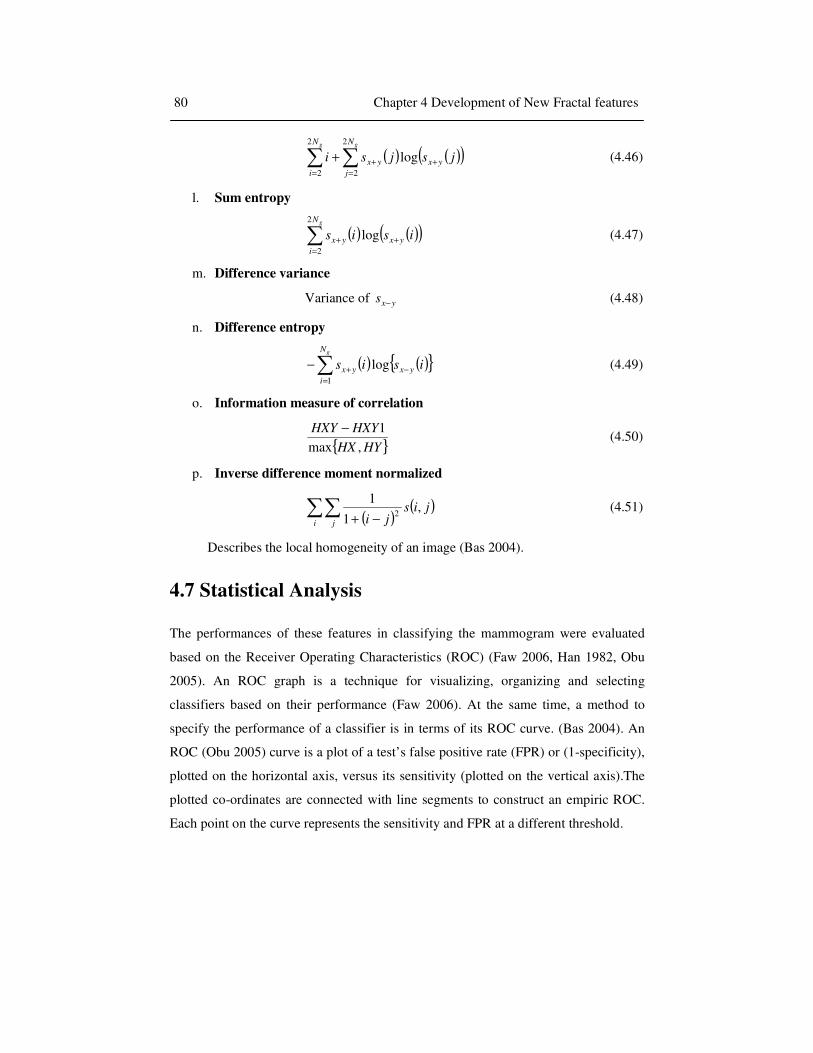
4.7 Statistical Analysis
The performances of these features in classifying the mammogram were evaluated
based on the Receiver Operating Characteristics (ROC) (Faw 2006, Han 1982, Obu
2005). An ROC graph is a technique for visualizing, organizing and selecting
classifiers based on their performance (Faw 2006). At the same time, a method to
specify the performance of a classifier is in terms of its ROC curve. (Bas 2004). An
ROC (Obu 2005) curve is a plot of a test’s false positive rate (FPR) or (1-specificity),
plotted on the horizontal axis, versus its sensitivity (plotted on the vertical axis).The
plotted co-ordinates are connected with line segments to construct an empiric ROC.
Each point on the curve represents the sensitivity and FPR at a different threshold.
80 Chapter 4 Development of New Fractal features

56 Chapter 4. Development of New Fractal Features
An ROC curve begins at the (0, 0) co-ordinate, corresponding to the strictest
decision threshold whereby all test results are negative for disease. The ROC ends at
the (1,1) co-ordinates corresponding to the most lenient decision threshold whereby
all test results are positive for disease.
The line connecting the (0, 0) and (1, 1) co-ordinates is called the “chance
diagonal” and represents the ROC curve of diagnostic test with no ability to
distinguish patients with and without disease. The farther away an ROC curve from
the chance diagonal, the closer to the upper left hand corner, the better the
discriminating power and the diagnostic accuracy of the test is.
The area under the curve (AUC) is an accepted modality for comparing
classifier performance. A perfect classifier has TP rate of 1.0, and an FP rate of 0.0,
resulting in an AUC of 1.0.The most popular measure of accuracy is the Area under
the ROC curves denoted by AUC which ranges from the value 0.5 (chance) to 1.0
(perfect discrimination or accuracy). Another measure to summarize accuracy is the
Youden’s index, defined as sensitivity + specificity-1. There is another measure
called the accuracy. It is shown that the probability of a correct diagnosis is
equivalent to
Probability (correct diagnosis) =PREVs × sensitivity + (1- PREVs) ×
specificity. where PREVs is the prevalence of disease in the sample.
Thus an ROC demonstrates several things:
• Shows the trade-off between sensitivity and specificity.
• The closer the curve approaches to the left hand border of the top border
of the ROC space, the more accurate the test.
• The closer the curve comes to the 450 diagonal of the ROC space, the less
accurate the test.
• The AUC for an ideal classifier is 1 (Bas 2004).
4.7 Statistical Analysis 81

56 Chapter 4. Development of New Fractal Features
4.8 Implementation of Classification of Mammograms
using various fractal features
The various features mentioned above were evaluated and the results are
mentioned in the following sections.
4.8.1 Database used
The mammograms used for validating the above discussed methods were obtained
from the freely available two standard online mammogram research databases
namely, Mammogram Image Analysis Society (MIAS) and Digital Database for
Screening Mammography (DDSM).
4.8.1.1 MIAS Database
The images in the MIAS database are digitized at a resolution of 50 µm per pixel,
with 1,024×1,024 pixel size and at 256 gray levels (Suc 1994). The accompanied
“ground truth” contains details regarding the character of the background tissue,
class, and severity of the abnormality and x, y coordinate of its center and radii. The
size of microcalcification generally varies from 50 to 1,000µm. The smallest
microcalcification is equivalent to 1 pixel of the image. The subtlety rating of these
mammograms are found to be 1, 2, and 3 as per (Pis 1998) which indicates that the
lesions are detectable only by an expert mammographer, likely to be detected by an
expert, and likely to be detected by observer with good mammographic training,
respectively.
4.8.1.2 DDSM Database
The DDSM contains mammograms obtained from Massachusetts General Hospital,
Wake Forest University School of Medicine, Sacred Heart Hospital and Washington
University of St. Louis School of Medicine. The four standard views (medio-lateral
oblique and cranio caudal) from each case were digitized on one of four different.
82 Chapter 4 Development of New Fractal features

56 Chapter 4. Development of New Fractal Features
The cases were all from mammography examinations conducted between October of
1988 and February of 1999.
The cases were assigned to volumes according to the severity of the finding.
‘Normal’ volumes contain mammograms from screening exams that were read as
‘normal’ and had a normal screening exam four years later (plus or minus 6 months).
‘Benign without callback volumes’ contain examined mammograms that had an
abnormality that was noteworthy but did not require the patient to be recalled for any
additional workup. ‘Benign’ volumes contain cases in which something suspicious
was found and the patient was recalled for some additional work-up that resulted in a
benign finding. ‘Cancer’ volumes contain cases in which a histologically proven
cancer was found. Each volume may contain cases that include less severe findings in
addition to the more severe findings that resulted in the assignment of a case to a
particular volume.
Every case in the DDSM contains the patient age, the screening exam date,
the date on which the mammograms were digitized and the ACR breast density, that
was specified by an expert radiologist. Cases in all volumes other than the normal
volume contain pixel level ground truth markings of abnormalities. Each marking
contains a subtlety value and a description that was specified by an expert
mammography radiologist using the BI-RADS™ (ACR 1998) lexicon (Hea 2001).
The following table 4.1 shows the number of mammograms from the two
databases used for the study.
Table 4.1 No of Mammograms of each class obtained from the MIAS and DDSM Database used for the study
Type of Mammogram MIAS DDSM
Normal 166 180
Masses Benign 54 84
Malignant 39 75
Microcalcifications Benign 13 87
Malignant 15 86
Total 287 512
4.8 Implementation of Classification of Mammograms 83

56 Chapter 4. Development of New Fractal Features
4.9 Results and Discussions
Different Regions of Interest (ROI) viz. 64 × 64, 128 × 128, 256 × 256, were chosen
from the mammogram, depending on the radius of the cancerous region present in the
image. In the normal mammograms also same size for regions of interest were
considered.
4.9.1 Evaluation using fractal signatures and distance measures
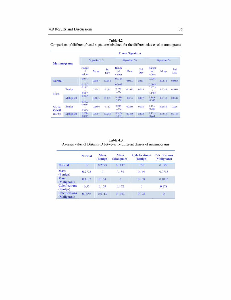
The fractal signatures computed according to sections 4.4.3.1 and 4.4.3.2 for the
different class of mammograms are shown in the table 4.2. The values of the
signatures S, S+ and S- obtained for normal mammograms, mammograms with
microcalcifications and masses which are both benign and malignant are shown in the
table. For normal mammograms the average values of the signatures are the lowest,
with 0.0887, 0.0863 and 0.0632 for S, S+ and S- respectively. But, the range of values
for one class overlap with the values of other classes, for all the fractal signatures S,
S+ and S- and hence cannot be used efficiently for classification of mammograms. The
average standard deviation and range of these values is also given in the table 4.2.
Next, the distance D between the different classes of mammograms based on
equation (4.12) was measured. The table 4.3 shows the average value of the distance D
obtained between the different classes of mammograms. It is seen from the table that
there is sufficient distance between different classes, except for normal and malignant
microcalcifications, which is found to be very less of 0.0556. The distance between
normal and other classes should be high because when abnormality is present, it
should be detected correctly. Hence, this distance measure D cannot be used as a good
classifier for characterizing mammograms.
84 Chapter 4 Development of New Fractal features
56 Chapter 4. Development of New Fractal Features
Table 4.2
Comparison of different fractal signatures obtained for the different classes of mammograms
Mammograms
Fractal Signatures
Signature S Signature S+ Signature S-
Range of
values Mean
Std Dev
Range of
values Mean
Std Dev
Range of
values Mean
Std Dev
Normal 0.0347
-0.1267
0.0887 0.0051 0.0323
-0.0967
0.0863 0.0197 0.0291
-0.0863
0.0632 0.0015
Mass
Benign 0.1165
-0.3439
0.1347 0.134 0.197-0.382
0.2915 0.026 0.1573
-0.4382
0.3743 0.1068
Malignant 0.2709
-0.3722
0.3135 0. 135 0.168-0.356
0.274 0.0839 0.149-0.385
0.2733 0.0547
Micro
Calcifi
cations
Benign 0.0684
-0.3906
0.2569 0.112 0.203-0.342
0.2258 0.021 0.155-0.286
0.1988 0.016
Malignant 0.658-0.8319
0.7087 0.0285 0.316-0.355
0.3445 0.0095 0.121-0.661
0.3553 0.3118
Table 4.3
Average value of Distance D between the different classes of mammograms
Normal Mass
(Benign)
Mass
(Malignant)
Calcifications
(Benign)
Calcifications
(Malignant)
Normal 0 0.2793 0.1137 0.55 0.0556
Mass
(Benign) 0.2793 0 0.154 0.169 0.0713
Mass
(Malignant) 0.1137 0.154 0 0.158 0.1033
Calcifications
(Benign) 0.55 0.169 0.158 0 0.178
Calcifications
(Malignant) 0.0556 0.0713 0.1033 0.178 0
4.9 Results and Discussions 85

56 Chapter 4. Development of New Fractal Features
Table 4.4 illustrates the differential distance D’ computed using equation
(4.15). There is ample variation in the differential distance measure between the
normal and the abnormal mammograms.
Table 4.4 Differential Distance D’ between the different classes of mammograms
But the differential distance D’ cannot identify exactly to which class a
mammogram belongs. Therefore, it was not possible to generalize and categorize the
class of mammograms using this distance measure D’.
4.9.2. Evaluation of Fractal Dimension Estimated from
different methods
The fractal dimensions of the mammograms were calculated using the
Triangular Prism Surface Area method (TPSA), Differential Box Counting (DBC)
method and the blanket method. For an ROI of M ×M, in the TPSA method and the
DBC methods an overlapping grid size of 1 to M were considered. For the blanket
method, blanket size ε was varied from 0 to 20.The results obtained are given in table
4.5.
Normal Mass
(Benign)
Mass
(Malignant)
Calcifications
(Benign)
Calcifications
(Malignant)
Normal 0 0.583 0.3171 0.213 0.2189
Mass
(Benign) 0.583 0 0.2833 0.1311 0.6198
Mass
(Malignant) 0.3171 0.2833 0 0.588 0.2702
Calcifications
(Benign) 0.213 0.1311 0.588 0 0.552
Calcifications
(Malignant) 0.2189 0.6198 0.2702 0.552 0
86 Chapter 4 Development of New Fractal features
56 Chapter 4. Development of New Fractal Features
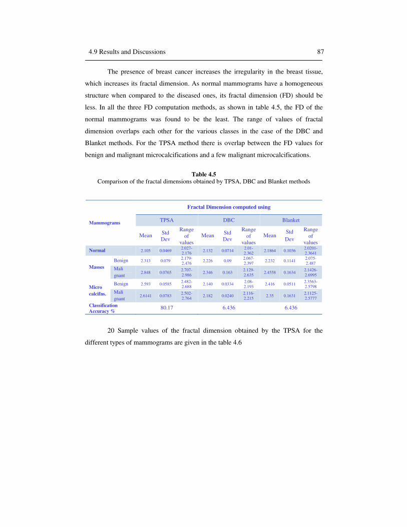
The presence of breast cancer increases the irregularity in the breast tissue,
which increases its fractal dimension. As normal mammograms have a homogeneous
structure when compared to the diseased ones, its fractal dimension (FD) should be
less. In all the three FD computation methods, as shown in table 4.5, the FD of the
normal mammograms was found to be the least. The range of values of fractal
dimension overlaps each other for the various classes in the case of the DBC and
Blanket methods. For the TPSA method there is overlap between the FD values for
benign and malignant microcalcifications and a few malignant microcalcifications.
Table 4.5
Comparison of the fractal dimensions obtained by TPSA, DBC and Blanket methods
20 Sample values of the fractal dimension obtained by the TPSA for the
different types of mammograms are given in the table 4.6
Mammograms
Fractal Dimension computed using
TPSA DBC Blanket
Mean Std Dev
Range of
values
Mean Std Dev
Range of
values
Mean Std
Dev
Range of
values
Normal 2.105 0.0469 2.027-2.176
2.132 0.0714 2.01-2.362
2.1864 0.1036 2.0201-2.3641
Masses
Benign 2.313 0.079 2.179-2.476
2.226 0.09 2.067-2.397
2.232 0.1141 2.075-2.487
Mali
gnant 2.848 0.0765
2.707-2.986
2.346 0.163 2.129-2.635
2.4558 0.1634 2.1426-2.6995
Micro
calcifns.
Benign 2.593 0.0585 2.482-2.688
2.140 0.0334 2.08-2.193
2.416 0.0511 2.3563-2.5798
Mali
gnant 2.6141 0.0783
2.502-2.764
2.182 0.0240 2.116-2.215
2.35 0.1631 2.1125-2.5777
Classification
Accuracy % 80.17 6.436 6.436
4.9 Results and Discussions 87

56 Chapter 4. Development of New Fractal Features
Table 4.6
Sample Fractal Dimension obtained for different mammograms using TPSA method
Sl. No Normal Masses Microcalcifications
Benign Malignant Benign Malignant
1 2.06 2.476 2.841 2.606 2.644
2 2.116 2.299 2.713 2.557 2.538
3 2.027 2.179 2.947 2.688 2.676
4 2.094 2.451 2.942 2.647 2.523
5 2.086 2.402 2.804 2.6027 2.615
6 2.105 2.394 2.754 2.564 2.592
7 2.152 2.357 2.824 2.546 2.502
8 2.085 2.289 2.952 2.579 2.616
9 2.04 2.208 2.942 2.65 2.568
10 2.175 2.37 2.788 2.482 2.683
11 2.145 2.225 2.857 2.565 2.604
12 2.075 2.303 2.986 2.669 2.585
13 2.052 2.298 2.897 2.547 2.6075
14 2.169 2.385 2.857 2.55 2.567
15 2.052 2.315 2.751 2.58 2.589
16 2.169 2.387 2.766 2.654 2.654
17 2.052 2.289 2.745 2.67 2.764
18 2.056 2.342 2.8 2.482 2.669
19 2.064 2.284 2.874 2.52 2.511
20 2.165 2.216 2.849 2.53 2.717
4.9.2.1. Box Plot of Fractal Dimensions
Box plot, also known as whisker plot is a convenient way of graphically depicting
groups of numerical data. The main characteristics of this plot are the following:
• The tops and bottoms of each "box" are the 25th and 75th percentiles
of the samples, respectively. The distances between the tops and
bottoms are the interquartile ranges.
88 Chapter 4 Development of New Fractal features

56 Chapter 4. Development of New Fractal Features
• The line in the middle of each box is the sample median. If the
median is not centered in the box, it shows sample skewness.
• The whiskers are lines extending above and below each box.
Whiskers are drawn from the ends of the interquartile ranges to the
furthest observations within the whisker length (the adjacent values).
• Observations beyond the whisker length are marked as outliers. In
the figure, outliers are displayed with a red + sign.
• Notches display the variability of the median between samples.
Box plots of fractal dimension obtained using different methods TPSA,
Blanket and DBCM are shown in fig. 4 .6.
(a)TPSA
4.9 Results and Discussions 89
(b) DBCM
Outliers
Whiskers
Median

56 Chapter 4. Development of New Fractal Features
It is clear from fig. 4.6(a), that for the TPSA method, the range of FD values
for a few malignant masses and microcalcifications (both benign and malignant) are
overlapping, so these categories cannot be correctly classified. In fig. 4.6(b), for
DBCM, FD values of all the categories are overlapping each other, but the highest
value was obtained for malignant mass and minimum value was obtained for the
normal mammograms. Similar was the case with the blanket method shown in fig.
4.6(c).
4.9.2.2 Classification Accuracy using Fractal Dimension
The classification accuracy is the ratio of the number mammograms which are
correctly classified to the total number of mammograms considered; both normal and
cancerous. The table 4.7 shows the number of mammograms which are correctly
classified in each database. In the TPSA method, the ranges of individual FD values
were not overlapping for normal and benign and malignant masses. Therefore it was
possible to correctly classify these categories with 100% accuracy.
But the range of FD values for benign and malignant microcalcifications
were overlapping with the other categories. For the MIAS database, 166 Normal, 54
(c) Blanket
Fig. 4.6 Box Plot of the Fractal Dimension obtained using TPSA, DBCM and
Blanket methods
90 Chapter 4 Development of New Fractal features

56 Chapter 4. Development of New Fractal Features
masses (benign) and 39 masses (malignant) were classified accurately, thus the
classification accuracy becomes %24.90287259 = .
Table 4.7
Mammograms correctly classified using fractal dimension computed using TPSA, DBC and Blanket methods
Database
No. of Mammograms correctly classified by Fractal Dimension
Computed using
TPSA DBC Blanket
Normal Mass (Ben)
Mass (Malig.)
Normal Mass
(Malig) Normal
Mass (Malig)
MIAS (287 Nos) 166 54 39 13 9 14 8
DDSM (512 Nos) 180 84 75 21 14 21 14
Overall
Classification
accuracy%
74.84 7.1339 7.1339
With the DDSM database, 180 normal, 84 masses (benign) and 75 masses
(malignant) were correctly classified and the classification accuracy obtained
was %21.66512339 = . Thus the overall classification accuracy becomes 74.84%. As
seen from table 4.5, in the DBC method, the range of FD values of various classes
overlap each other. Only 9 malignant masses and 13 normal ones from the MIAS
database and 14 malignant and 21 normal from the DDSM database were classified
correctly using DBCM, giving a classification accuracy of 7.1339% only. Similar was
the case with blanket method. Only 22 (14 normal and 8 malignant masses) from
MIAS and 35 (21 normal and 14 malignant) from the DDSM databases could be
accurately classified and the classification accuracy obtained was again 7.1339%.
It may be noted that, in the TPSA method, four experimental points
considered at a time are forming a quadruple and this quadruple are covered by four
triangles with mean elevation of four vertices as the common central point. When
smaller triangular tiles are considered, they are not in simple relation with the cross
section of the base of the prism, but also depend on the properties of the surface itself.
Thus, TPSA method can provide an accurate measurement of fractal dimension
4.9 Results and Discussions 91

56 Chapter 4. Development of New Fractal Features
compared to the DBCM and blanket method. The latter two methods are similar, with
the difference of the gray level surface is been considered for computing the fractal
dimension.
As the classification accuracy for the feature FD is low as mentioned above,
the six fractal features, 1f -
6f described in section 4.5 were calculated using the three
FD estimation methods. They were found to provide better classification accuracy.
4.9.3 Evaluation using Fractal Features 1f - 6f
The results obtained while computing the fractal features (1f -
6f ) of
malignant mass, benign mass, malignant and benign microcalcifications, and normal
mammograms using the three methods are described in the following sections.
4.9.3.1 Evaluation using Fractal Feature 1f
Different overlapping window sizes were chosen to compute feature1f , but
window of size of 2 gave good results. The feature images obtained using equation
(4.24) to extract fractal feature 1f is shown in fig. 4.7. The range of values, mean and
standard deviation of f1 computed using TPSA, DBCM and blanket method are
shown in table 4.8. For the TPSA method, there was ample separation between the
values for normal and cancerous mammograms, but the range of values for the classes
overlap. For the other two methods ‘f1’ values overlap between all classes.
The sample values of fractal feature f1 obtained for 20 mammograms each
from various classes, using the TPSA method, is presented in table 4.9.
The box plot for fractal feature1f obtained using TPSA; DBCM and Blanket
methods are given in fig.4.8 (a)-(c) respectively. The results as analyzed in table 4.8
can be visualized in the box plot. The table 4.10 shows the number of mammograms
which are correctly classified in each database. Table shows that none of the
mammograms were classified correctly by DBC method as all the individual feature
values were overlapping with other classes.
92 Chapter 4 Development of New Fractal features

56 Chapter 4. Development of New Fractal Features
.
Fig. 4.7 Fractal feature image of Malignant Mass, Benign Mass, Benign Microcalcifications, Malignant Microcalcifications, Normal Mammograms respectively for computing feature f1
In blanket method also, as seen from the box plot fig. 4.8(c) feature values of all the
classes of mammograms were overlapping, giving an accuracy of only 1.877% as
Malignant Mass Benign Mass
Benign Microcalcifications Malignant Microcalcifications
Normal
4.9 Results and Discussions 93

56 Chapter 4. Development of New Fractal Features
only 15 malignant masses were classified correctly. In the TPSA method, 296 out of
344 normal and 93 out of 252 masses were correctly detected giving a classification
accuracy of 48.6858.
Table 4.8
Comparison of the fractal feature 1f obtained using TPSA, DBC and Blanket Methods
Mammograms
Fractal feature 1f computed using
TPSA DBC Blanket
Range of
values
Mean Std Dev
Range of
values
Mean Std Dev
Range of
values
Mean Std Dev
Normal 0.002 -
0.223 0.1217 0.0668
0.153-0.451
0.2900 0.0863 0.0432-0.2963
0.1771 0.0746
Masses Benign 0.312 -
0.784 0.5087 0.1621
0.046-0.299
0.1662 0.0892 0.0182-0.3445
0.1711 0.0845
Malign. 0.372 -
0.879 0.658 0.1161
0.171-0.235
0.2110 0.0163 0.1611-0.3752
0.2682 0.0598
Microcalci
fications
Benign 0.411 -
0.688 0.5578 0.0895
0.21-0.432
0.3288 0.0669 0.0787-0.3047
0.2392 0.0525
Malign. 0.411 -
0.763 0.6201 0.1059
0.266-0.398
0.3264 0.0375 0.1692-0.3367
0.2624 0.0504
Classification
Accuracy % 48.6858 0 1.877
94 Chapter 4 Development of New Fractal features

56 Chapter 4. Development of New Fractal Features
Table 4.9 Sample Fractal feature f1 values obtained for different mammograms using TPSA
method
Sl. No Normal Masses Microcalcifications
Benign Malignant Benign Malignant
1 0.157 0.689 0.78 0.678 0.525
2 0.002 0.487 0.703 0.501 0.457
3 0.115 0.312 0.568 0.566 0.638
4 0.099 0.45 0.372 0.452 0.712
5 0.119 0.346 0.781 0.517 0.411
6 0.067 0.55 0.703 0.533 0.653
7 0.102 0.559 0.6763 0.607 0.689
8 0.102 0.335 0.695 0.632 0.608
9 0.095 0.378 0.527 0.599 0.66
10 0.054 0.356 0.622 0.683 0.601
11 0.168 0.452 0.604 0.663 0.644
12 0.07 0.528 0.534 0.632 0.73
13 0.19 0.436 0.738 0.6045 0.696
14 0.19 0.337 0.632 0.5744 0.707
15 0.002 0.369 0.671 0.411 0.6247
16 0.053 0.457 0.748 0.523 0.711
17 0.15 0.784 0.538 0.681 0.732
18 0.127 0.599 0.392 0.532 0.634
19 0.143 0.641 0.592 0.59 0.677
20 0.17 0.45 0.709 0.621 0.431
(a)TPSA
4.9 Results and Discussions 95

56 Chapter 4. Development of New Fractal Features
Table 4.10 Mammograms Classification using Fractal feature f1 computed using TPSA, DBC and Blanket
methods
Database
No. of Mammograms Classified Correctly by
Fractal feature f1 Computed using
TPSA DBC Blanket
Normal Mass (Ben)
Mass (Malig.)
- Mass (Malig)
MIAS(287 Nos) 126 15 11 - 5
DDSM(512 Nos) 170 36 31 - 10
Overall
Classification
accuracy%
48.6858 0 1.877
Fig. 4.8 Box Plot of the feature f1obtained using TPSA, DBCM and Blanket methods
(b)DBCM
(c)Blanket
96 Chapter 4 Development of New Fractal features

56 Chapter 4. Development of New Fractal Features
4.9.3.2 Evaluation using Fractal Feature 2f
The high gray valued images obtained using equation (4.25), for the different
categories of mammograms are shown in fig.4.9. Table 4.11 illustrates the
comparison of the fractal feature 2f values obtained for different methods. In the
TPSA method, the maximum value for feature 2f was obtained for the malignant
mammograms while minimum was obtained for the normal mammogram, as
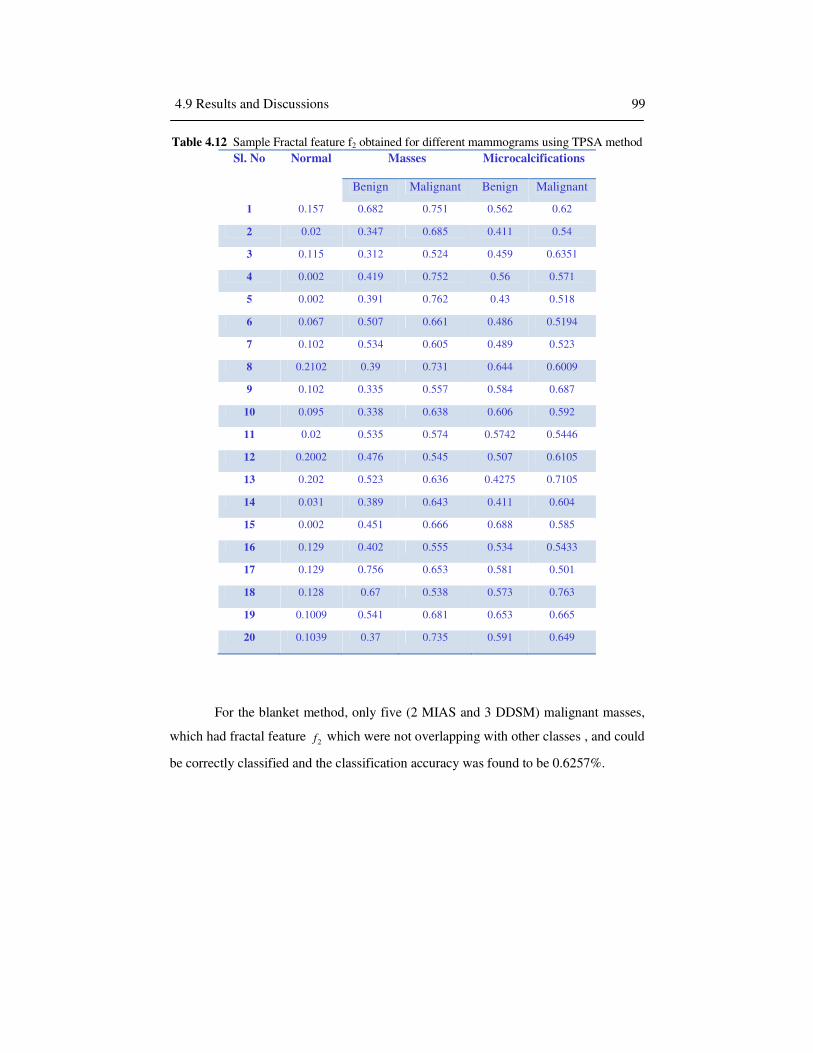
required. Sample feature 2f values obtained by the TPSA method are shown in table
4.12. The spread of the fractal feature 2f values are illustrated in the box plot fig.
4.10. As seen from box plot 4.10(a), none of the individual values of feature f2 for
normal mammograms were overlapping with other classes, but all the other classes
had overlapping values. Therefore, all normal mammograms and few masses were
correctly classified by feature f2 , obtained by TPSA method.
Malignant Mass Benign Mass
Benign Microcalcifications Malignant Microcalcifications
4.9 Results and Discussions 97

56 Chapter 4. Development of New Fractal Features
Fig.4.9 Fractal feature image of Malignant Mass, Benign Mass, Benign Microcalcifications, Malignant Microcalcifications, Normal Mammograms respectively for computing feature f2
For the DBC method, benign masses had the lowest value for the feature 2f ,
but this cannot be considered as correct evaluation as benign mammograms have more
irregularity than normal ones. Therefore, 2f should be higher for benign than for
normal. Only 27 (7 MIAS and 20 DDSM) malignant masses were classified correctly
and the overall classification accuracy was only 3.379%.
Table 4.11
Comparison of the fractal feature 2f obtained using TPSA, DBC and Blanket
Methods
Mammograms
Fractal feature 2f computed using
TPSA DBC Blanket
Range of
values
Mean Std Dev
Range of
values
Mean Std Dev
Range of
values
Mean Std Dev
Normal 0.002-0.223
0.1201 0.0788 0.153-0.451
0.296 0.0843 0.043-0.296
0.190 0.1
Masses Benign 0.312-0.784
0.4962 0.1371 0.046-0.299
0.1707 0.0703 0.018-0.345
0.218 0.15
Malignant 0.524-0.879
0.6465 0.5585 0.171-0.635
0.3788 0.1397 0.161-0.375
0.264 0.069
Microc
alcifica
tions
Benign 0.411-0.688
0.5585 0.0776 0.21-0.432
0.3274 0.0620 0.221-0.339
0.290 0.183
Malignant 0.501-0.763
0.6197 0.0698 0.266-0.397
0.3426 0.0355 0.221-0.361
0.263 0.073
Classification
Accuracy %
46.433 3.379 0.6257
Normal
98 Chapter 4 Development of New Fractal features
56 Chapter 4. Development of New Fractal Features
Table 4.12 Sample Fractal feature f2 obtained for different mammograms using TPSA method
Sl. No Normal Masses Microcalcifications
Benign Malignant Benign Malignant
1 0.157 0.682 0.751 0.562 0.62
2 0.02 0.347 0.685 0.411 0.54
3 0.115 0.312 0.524 0.459 0.6351
4 0.002 0.419 0.752 0.56 0.571
5 0.002 0.391 0.762 0.43 0.518
6 0.067 0.507 0.661 0.486 0.5194
7 0.102 0.534 0.605 0.489 0.523
8 0.2102 0.39 0.731 0.644 0.6009
9 0.102 0.335 0.557 0.584 0.687
10 0.095 0.338 0.638 0.606 0.592
11 0.02 0.535 0.574 0.5742 0.5446
12 0.2002 0.476 0.545 0.507 0.6105
13 0.202 0.523 0.636 0.4275 0.7105
14 0.031 0.389 0.643 0.411 0.604
15 0.002 0.451 0.666 0.688 0.585
16 0.129 0.402 0.555 0.534 0.5433
17 0.129 0.756 0.653 0.581 0.501
18 0.128 0.67 0.538 0.573 0.763
19 0.1009 0.541 0.681 0.653 0.665
20 0.1039 0.37 0.735 0.591 0.649
For the blanket method, only five (2 MIAS and 3 DDSM) malignant masses,
which had fractal feature 2f which were not overlapping with other classes , and could
be correctly classified and the classification accuracy was found to be 0.6257%.
4.9 Results and Discussions 99

56 Chapter 4. Development of New Fractal Features
(a)TPSA
(b)DBCM
(c)Blanket Fig. 4.10 Box Plot of the feature f2 obtained using TPSA, DBCM and Blanket
methods
100 Chapter 4 Development of New Fractal features

56 Chapter 4. Development of New Fractal Features
The actual number of mammograms which were correctly classified in each
database, using the different methods is shown in table 4.13.
Table 4.13
Mammograms correctly classified using Fractal feature f2 computed using TPSA, DBC and Blanket methods
Database
No. of Mammograms Classified Correctly by
Fractal feature f2 Computed using
TPSA DBC Blanket
Normal Mass (Ben)
Mass (Malig.)
Mass (Malig)
Mass (Malig)
MIAS (287 Nos) 166 7 4 7 2
DDSM (512 Nos) 180 10 4 20 3
Overall
Classification
accuracy%
46.433 3.379 0.6257
4.9.3.3 Evaluation using Fractal Feature 3f
The low gray level feature images computed using equation (4.26) for finding fractal
feature 3f is shown in fig.4.11. As seen in fig.4.11, no structures of the mammograms
are present in the 3f feature image and hence no details about the structure will be
obtained from this feature3f . This is evident from the values shown in table 4.14,
which gives the comparison of f3 feature values obtained using the three methods.
Table 4.14 shows that the values of the fractal feature3f , are in the same range for the
different classes of mammograms, for all the three methods and these values are
found to be very small. This is because irregularity in the low gray level image is less.
The sample values of fractal feature f3 obtained for the different classes of mammo-
4.9 Results and Discussions 101

56 Chapter 4. Development of New Fractal Features
grams using the TPSA method is presented in table 4.15. The box plot given in
fig.4.12 also indicates that all the categories of mammograms are having values in the
same range.
Fig.4.11 Fractal feature image of Malignant Mass, Benign Mass, Benign Microcalcifications,
Malignant Microcalcifications, Normal Mammograms respectively for computing feature f3
Malignant Mass Benign Mass
Benign Microcalcifications Malignant Microcalcifications
Normal
102 Chapter 4 Development of New Fractal features

56 Chapter 4. Development of New Fractal Features
The least classification accuracy was obtained for this feature, with the values
being 1.5018%, 0% and 1.5018% for the TPSA, DBC and Blanket methods
respectively. Table 4.16 shows the number of mammograms which are correctly
classified in each database using the fractal feature f3.
Table 4.14
Comparison of the fractal feature 3f obtained using TPSA, DBC and Blanket Methods
Mammo
grams
Fractal feature 3f computed using
TPSA DBC Blanket
Range of
values
Mean Std Dev
Range of
values
Mean Std Dev
Range of
values
Mean Std Dev
Normal 0.003-0.365 0.2532 0.1096
0.144-0.531
0.347 0.1297 0-0.012 0.0071 0.0037
Masses Benign 0.203-0.506 0.2785 0.0841
0.074-0.368
0.1834 0.0975 0-0.12 0.01019 0.0187
Mali
gnant 0.007-0.598 0.2894 0.1515
0.077-0.492
0.244 0.115 0-0.1127 0.036 0.0458
Micro
calcific
ations
Benign 0. 06-0.262 0.125 0.065
0.074-0.251
0.184 0.0555 0-0.003 0.00142 0.00109
Mali
gnant 0.075-0.215 0.1324 0.0503 0.042-0.144
0.107 0.0294 0-0.007 0.0045 0.0022
Classification
Accuracy % 1.5018 0 1.5018
4.9 Results and Discussions 103

56 Chapter 4. Development of New Fractal Features
Table 4.15 Sample Fractal feature f3 obtained for different mammograms using TPSA method
Sl. No Normal Masses Microcalcifications
Benign Malignant Benign Malignant
1 0.315 0.468 0.138 0.262 0.215
2 0.365 0.203 0.497 0.075 0.075
3 0.315 0.21 0.215 0.075 0.211
4 0.365 0.207 0.215 0.0648 0.075
5 0.337 0.248 0.091 0.0754 0.193
6 0.253 0.203 0.453 0.067 0.075
7 0.2521 0.263 0.435 0.075 0.075
8 0.365 0.235 0.089 0.132 0.076
9 0.365 0.259 0.131 0.075 0.205
10 0.14 0.506 0.375 0.075 0.126
11 0.259 0.417 0.373 0.165 0.129
12 0.365 0.221 0.44 0.215 0.089
13 0.365 0.361 0.007 0.075 0.077
14 0.314 0.252 0.429 0.155 0.075
15 0.129 0.205 0.464 0.06 0.19
16 0.003 0.218 0.172 0.11 0.086
17 0.123 0.286 0.23 0.13 0.0944
18 0.365 0.289 0.215 0.124 0.104
19 0.221 0.241 0.159 0.09 0.15
20 0.2201 0.2065 0.133 0.091 0.201
(a)TPSA
104 Chapter 4 Development of New Fractal features

56 Chapter 4. Development of New Fractal Features
Table 4.16
Mammograms correctly classified using Fractal feature f3 computed using TPSA, DBC and Blanket methods
Database
No. of Mammograms Classified Correctly by
Fractal feature f3 Computed using
TPSA DBC Blanket
Normal Mass (Malig.)
- Mass
(Malig)
MIAS (287 Nos) 1 3 0 4
DDSM (512 Nos) 2 6 0 8
Overall
Classification
accuracy%
1.5018 0 1.5018
(b)DBCM
(c)Blanket
Fig 4.12 Box Plot of the feature f3 obtained using TPSA, DBCM and Blanket
methods
4.9 Results and Discussions 105

56 Chapter 4. Development of New Fractal Features
4.9.3.4 Evaluation using Fractal Feature 4f
The horizontally smoothed images computed using equation (4.28) for
finding the fractal feature 4f is given in fig.4.13. Value of feature f4 obtained using
the three different methods are given in tables 4.17. The box plot of the feature values
for the TPSA, DBC and Blanket methods are given in fig.4.14. The normal
mammograms and malignant masses had the lowest and highest feature4f values
respectively for the TPSA and DBC methods. But the standard deviation of this
feature for the malignant mass class were obtained as 0.105 and 0.1496 respectively
for the above two methods causing overlap between the classes. For the blanket
method, the values of the fractal feature 4f were in the same range for all the classes
of mammograms.
Malignant Mass Benign Mass
Benign Microcalcifications Malignant Microcalcifications
106 Chapter 4 Development of New Fractal features

56 Chapter 4. Development of New Fractal Features
Fig.4.13 Fractal feature image of Malignant Mass, Benign Mass, Benign Microcalcifications,
Malignant Microcalcifications, Normal Mammograms respectively for computing feature f4
As seen from table 4.17, the highest classification accuracy obtained for the
feature f4 was using the DBC method. Therefore, 20 sample values of fractal feature
f4 , obtained for different mammograms using DBC method are shown in table 4.18.
As shown in table 4.19, in TPSA, 26 normal (11 from MIAS and 15 from
DDSM) and 12 malignant masses (4 MIAS and 8 DDSM) were classified correctly.
Table 4.17
Comparison of the fractal feature 4f obtained using TPSA, DBC and Blanket Methods
Mammograms
Fractal feature 4f computed using
TPSA DBC Blanket
Range of
values
Mean Std Dev
Range of
values
Mean Std Dev
Range of
values
Mean Std Dev
Normal 0.018-0.173
0.0806 0.0449 0.055-0.582 0.2583 0.1297 0.0497-0.4771
0.325 0.1325
Masses Benign 0.167-0.681
0.3512 0.1258 0.218-0.44 0.332 0.0693 0.1298-0.5658
0.3375 0.1375
Mali gnant
0.337-0.72
0.4964 0.105 0.242-0.758 0.4667 0.1496 0.1039-0.4391
0.2598 0.1041
Micro
calcifi
cations
Benign 0.14-0.696
0.2566 0.1132 0.407-0.517 0.450 0.0384 0.3979-0.5919
0.481 0.0583
Mali gnant 0.068-
0.378 0.1881 0.0932 0.251-0.477 0.4049 0.0625
0.0822-0.4035
0.3036 0.0914
Classification
Accuracy % 4.755 16.2703 2.377
Normal
4.9 Results and Discussions 107

56 Chapter 4. Development of New Fractal Features
Highest mean value for the feature value was observed for malignant and the
least for normal mammograms. Even if there is enough separation between the mean
values of the different classes the individual values were spread between the classes
as observed in the box plot fig.4.14 (a).
With the DBC method, more number of normal mammograms (32 MIAS and
51 DDSM) and malignant masses (13- MIAS and 34 DDSM) were correctly
classified. Thus the overall classification accuracy with this feature was found to be
16.2703%. For this feature alone, DBCM gave the highest classification accuracy.
Table 4.18 Sample Fractal feature f4 obtained for different mammograms using DBC method
Sl. No Normal Masses Microcalcifications
Benign Malignant Benign Malignant
1 0.273 0.367 0.625 0.456 0.451
2 0.185 0.313 0.512 0.591 0.512
3 0.1009 0.329 0.765 0.539 0.5227
4 0.0118 0.3 0.656 0.532 0.47
5 0.213 0.344 0.59 0.547 0.3456
6 0.217 0.204 0.644 0.345 0.5119
7 0.235 0.298 0.51 0.3556 0.539
8 0.022 0.318 0.54 0.3689 0.3557
9 0.0213 0.272 0.759 0.4878 0.3497
10 0.104 0.3176 0.501 0.4876 0.3965
11 0.249 0.2954 0.746 0.4556 0.4853
12 0.345 0.2134 0.5667 0.4431 0.4467
13 0.344 0.2451 0.663 0.3782 0.4838
14 0.0321 0.3671 0.6689 0.3679 0.4253
15 0.361 0.3976 0.5691 0.3115 0.4735
16 0.0125 0.3566 0.7345 0.3968 0.4863
17 0.2781 0.3588 0.7293 0.4856 0.4291
18 0.121 0.3744 0.5792 0.4552 0.5003
19 0.125 0.408 0.5631 0.4483 0.5047
20 0.3712 0.3785 0.5741 0.5341 0.4931
108 Chapter 4 Development of New Fractal features

56 Chapter 4. Development of New Fractal Features
(a)TPSA
(b)DBCM
(c)Blanket
Fig. 4.14 Box Plot of the feature f4 obtained using TPSA, DBCM and
Blanket methods
4.9 Results and Discussions 109

56 Chapter 4. Development of New Fractal Features
Table 4.19
Mammograms correctly classified using Fractal feature f4 computed using TPSA, DBC and Blanket methods
In the blanket method, the benign microcalcifications produced the highest feature
values. Also normal and malignant microcalcifications had the least values which are
not correct according to the argument. Thus only 19 normal (5 MIAS and 14 DDSM)
mammograms were classified correctly with a classification accuracy of 2.377%.
4.9.3.5 Evaluation using Fractal Feature 5f
Fig.4.15 shows the vertically smoothed image obtained using equation (4.29)
for computing the fractal feature 5f , for the different classes of mammograms. The
feature values obtained for the three methods are tabulated in table 4.20. 20 sample
values of fractal feature f5 obtained for the different classes of mammograms using
the TPSA method is presented in table 4.21.
The spread of the feature values 5f is illustrated in the box plot shown in fig.
4.16. Normal and malignant masses had the lowest and highest feature 5f values
respectively for TPSA and DBC method. But these values were found to be
overlapping between other classes. In blanket method, the values are spread over all
the classes and could not distinguish between any class of mammograms as shown in
fig.4.16(a)-(c).The mean values also of normal, benign mass and malignant
microcalcifications were found to be in the same range for the blanket method.
Database
No. of Mammograms Classified Correctly by
Fractal feature f4 Computed using
TPSA DBC Blanket
Normal Mass (Malig.)
Normal Mass
(Malig.) Normal
MIAS (287 Nos) 11 4 32 13 5
DDSM (512 Nos) 15 8 51 34 14
Overall
Classification
accuracy%
4.755 16.2703 2.377
110 Chapter 4 Development of New Fractal features

56 Chapter 4. Development of New Fractal Features
Fig.4.15 Fractal feature image of Malignant Mass, Benign Mass, Benign Microcalcifications,
Malignant Microcalcifications, Normal Mammograms respectively for computing feature f5
Malignant Mass Benign Mass
Benign Microcalcifications Malignant Microcalcifications
Normal
4.9 Results and Discussions 111

56 Chapter 4. Development of New Fractal Features
Table 4.20
Comparison of the fractal feature 5f obtained using TPSA, DBC and Blanket Methods
Mammo
grams
Fractal feature 5f computed using
TPSA DBC Blanket
Range of
values
Mean Std Dev
Range of
values
Mean Std Dev
Range of
values
Mean Std Dev
Normal 0.005-0.156
0.0893 0.0497 0.113-0.342
0.237 0.0595 0.0603-0.5004
0.3475 0.1298
Masses Benign 0.119-0.357
0.2087 0.076 0.204-0.421
0.3342 0.0637 0.1025-0.4469
0.3173 0.089
Mali
gnant
0.331-0.72
0.4993 0.1053 0.194-0.727
0.4886 0.1218 0.0658-0.4485
0.2809 0.1094
Micro
calcific
ations
Benign 0.111-0.231
0.1777 0.0379 0.266-0.493
0.3873 0.0593 0.3944-0.567
0.4699 0.0450
Mali
gnant
0.146-0.419
0.2681 0.0856 0.293-0.524
0.4188 0.0647 0.1925-0.4628
0.3484 0.0729
Classification
Accuracy %
36.5456 19.0237 0
The number of mammograms which are correctly classified using feature f5 is
presented in table 4.22. Classification accuracies of 36.5456% (MIAS-normal (81),
malignant mass (24), DDSM-normal (115), malignant mass (72)), 19.0237% (MIAS-
normal (17), malignant mass (25), DDSM-normal (41), malignant mass (69)) and 0%
were obtained for TPSA, DBCM and Blanket methods respectively
112 Chapter 4 Development of New Fractal features

56 Chapter 4. Development of New Fractal Features
Table 4.21 Sample Fractal feature f5 obtained for different mammograms using TPSA method
Sl. No Normal Masses Microcalcifications
Benign Malignant Benign Malignant
1 0.119 0.241 0.578 0.127 0.146
2 0.005 0.121 0.595 0.125 0.191
3 0.118 0.121 0.383 0.111 0.219
4 0.0067 0.119 0.331 0.16 0.383
5 0.0067 0.123 0.561 0.169 0.235
6 0.0067 0.1478 0.535 0.2 0.146
7 0.09 0.2022 0.523 0.221 0.396
8 0.079 0.274 0.525 0.141 0.157
9 0.093 0.141 0.336 0.14 0.306
10 0.094 0.119 0.564 0.175 0.281
11 0.094 0.3514 0.497 0.22 0.1533
12 0.094 0.357 0.48 0.231 0.1689
13 0.094 0.188 0.453 0.138 0.419
14 0.0052 0.128 0.585 0.1925 0.186
15 0.0052 0.301 0.595 0.1807 0.1814
16 0.126 0.215 0.437 0.1922 0.345
17 0.145 0.348 0.384 0.1895 0.229
18 0.145 0.241 0.341 0.2134 0.3195
19 0.018 0.23 0.349 0.2094 0.381
20 0.032 0.247 0.52 0.2076 0.3445
(a)TPSA
4.9 Results and Discussions 113

56 Chapter 4. Development of New Fractal Features
Table 4.22
Mammograms correctly classified using Fractal feature f5 computed using TPSA, DBC and Blanket methods
Database
No. of Mammograms Classified Correctly by
Fractal feature f5 Computed using
TPSA DBC Blanket
Normal Mass (Malig.)
Normal Mass
(Malig.) -
MIAS (287 Nos) 81 24 17 25 -
DDSM (512 Nos) 115 72 41 69 -
Overall
Classification
accuracy%
36.5456 19.0237 -
Fig.4.16 Box Plot of the feature f5 obtained using TPSA, DBCM and
Blanket methods
(b)DBCM
(c)Blanket
114 Chapter 4 Development of New Fractal features

56 Chapter 4. Development of New Fractal Features
4.9.3.6 Evaluation using Fractal Feature 6f
As seen from the results in sections 4.9.3.1 to 4.9.3.5 none of the existing fractal
features f1 –f5 , were able to classify mammograms effectively. Hence the new fractal
feature 6f was developed from the average of four pixels as mentioned in equation
(4.30). The evaluation of f6 was done using TPSA, DBC and Blanket methods. It was
found that, rather than finding the difference between the minimum and maximum
gray level, in the DBCM method, and finding the volume of the blanket in the blanket
method, the area of the triangles formed by the height difference in the gray levels
gave better classification accuracy than the other two methods.
The images obtained for the different classes of mammograms, used for
calculating the fractal feature f6 are shown in fig.4.17. Table 4.23 illustrates the
feature values obtained by different methods. It is seen from the table that this feature
could classify the different types of mammograms more effectively and efficiently for
the TPSA method.
A set of 20 sample values of fractal feature f6, obtained for the different
classes of mammograms using the TPSA method is presented in table 4.24. The
spread of the fractal feature6f as seen in the box plot of fig.4.18(a)-(c) also projects
the same result. Analyzing the results for the TPSA method, it was seen that, there
was large separation between the 6f values and 100% classification was possible with
the 287 mammograms in MIAS database. For the 512 mammograms
4.9 Results and Discussions 115

56 Chapter 4. Development of New Fractal Features
Fig.4.17 Fractal feature image of Malignant Mass, Benign Mass, Benign Microcalcifications,
Malignant Microcalcifications, Normal Mammograms respectively for computing feature f6
Malignant Mass Benign Mass
Benign Microcalcifications Malignant Microcalcifications
Normal
116 Chapter 4 Development of New Fractal features
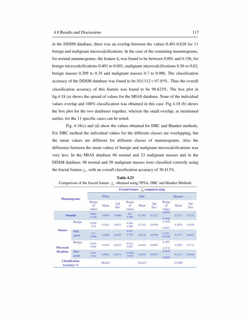
56 Chapter 4. Development of New Fractal Features
in the DDSM database, there was an overlap between the values 0.401-0.628 for 11
benign and malignant microcalcifications. In the case of the remaining mammograms,
for normal mammograms, the feature f6 was found to be between 0.001 and 0.156, for
benign microcalcifications 0.401 to 0.601, malignant microcalcifications 0.56 to 0.62,
benign masses 0.209 to 0.35 and malignant masses 0.7 to 0.986. The classification
accuracy of the DDSM database was found to be %85.97512501 = . Thus the overall
classification accuracy of this feature was found to be 98.623%. The box plot in
fig.4.18 (a) shows the spread of values for the MIAS database. None of the individual
values overlap and 100% classification was obtained in this case. Fig 4.18 (b) shows
the box plot for the two databases together, wherein the small overlap, as mentioned
earlier, for the 11 specific cases can be noted.
Fig. 4.18(c) and (d) show the values obtained for DBC and Blanket methods.
For DBC method the individual values for the different classes are overlapping, but
the mean values are different for different classes of mammograms. Also the
difference between the mean values of benign and malignant microcalcifications was
very less. In the MIAS database 66 normal and 23 malignant masses and in the
DDSM database, 96 normal and 58 malignant masses were classified correctly using
the fractal feature6f , with an overall classification accuracy of 30.413%.
Table 4.23
Comparison of the fractal feature 6f obtained using TPSA, DBC and Blanket Methods
Mammograms
Fractal feature 6f computed using
TPSA DBC Blanket
Range of
values Mean
Std Dev
Range of
values Mean
Std Dev
Range of
values Mean
Std Dev
Normal 0.001-0.156
0.0934 0.0485 0.0-
0.388 0.1783 0.1221
0.0508-
0.3646 0.1773 0.1232
Masses
Benign 0.209-0.35
0.2841 0.0471 0.204-0.408
0.3142 0.0549 0.1029
-0.4471
0.2078 0.1036
Mali
gnant 0.7-
0.986 0.8269 0.0785
0.501-
0.765 0.6178 0.0796 0.126-0.5258
0.3777 0.6612
Microcalc
ifications
Benign 0.401-0.601
0.4497 0.0327 0.312-0.591
0.4454 0.0807 0.1603
-0.5778
0.2930 0.1731
Mali
gnant 0.56-0.62
0.5861 0.0171 0.3456-0.539
0.4516 0.0535 0.1678
-0.2918
0.2311 0.0616
Classification
Accuracy % 98.623 30.413 23.905
4.9 Results and Discussions 117
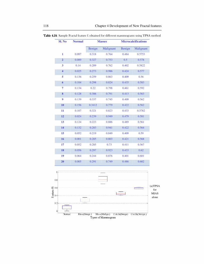
56 Chapter 4. Development of New Fractal Features
Table 4.Table 4.Table 4.Table 4.24242424 Sample Fractal feature f6 obtained for different mammograms using TPSA method
Sl. No Normal Masses Microcalcifications
Benign Malignant Benign Malignant
1 0.097 0.318 0.764 0.484 0.5753
2 0.089 0.327 0.753 0.5 0.578
3 0.14 0.209 0.762 0.402 0.5822
4 0.025 0.273 0.986 0.424 0.577
5 0.136 0.259 0.863 0.409 0.56
6 0.104 0.298 0.824 0.435 0.583
7 0.134 0.22 0.798 0.461 0.592
8 0.128 0.306 0.791 0.413 0.563
9 0.139 0.337 0.745 0.409 0.562
10 0.156 0.3412 0.779 0.422 0.562
11 0.107 0.321 0.823 0.433 0.5782
12 0.024 0.239 0.949 0.479 0.581
13 0.124 0.223 0.886 0.489 0.561
14 0.132 0.283 0.941 0.422 0.564
15 0.052 0.219 0.849 0.409 0.59
16 0.001 0.285 0.803 0.421 0.568
17 0.052 0.285 0.73 0.411 0.567
18 0.056 0.297 0.923 0.433 0.62
19 0.064 0.244 0.876 0.401 0.601
20 0.005 0.291 0.749 0.486 0.602
(a)TPSA
for
MIAS
alone
118 Chapter 4 Development of New Fractal features

56 Chapter 4. Development of New Fractal Features
(b) DBCM
(c)Blanket
Fig. 4.18 Box Plot of the feature f6 obtained using TPSA, DBCM and
Blanket methods for MIAS and DDSM together
4.9 Results and Discussions 119
(b) TPSA
for MIAS
and DDSM

56 Chapter 4. Development of New Fractal Features
Table 4.25 Mammograms correctly classified using Fractal feature f6 computed using TPSA, DBC and Blanket methods
Database
No. of Mammograms Classified Correctly by
Fractal feature f6 Computed using
TPSA DBC Blanket
Normal Mass
(Malig.) Normal
MIAS (287 Nos) All mammograms 66 23 87
DDSM (512 Nos) All except 11 benign microcalcifications
96 58 104
Overall
Classification
accuracy%
98.623 30.413 23.905
In the blanket method only the normal mammograms were classified
accurately. 87 from MIAS and 104 from the DDSM database were categorized
correctly effectively by this feature, giving an overall accuracy of 23.905%. Table
4.25 illustrates the classification accuracies obtained this feature using different
methods.
From the above evaluations, it can be concluded that fractal feature 6f
obtained by the TPSA method is the best feature for classifying the different classes
of mammograms with a total classification accuracy of 98.623%. But the range of 6f
between benign and malignant microcalcifications is less and so, other features may
be added for better estimation, if needed.
4.9.4 Performance Evaluation of the Features
A good feature must be sufficiently discriminating. It was seen that the classification
accuracy is the highest with the feature 6f computed using the TPSA method. These
performances were evaluated using the freely available software MedCalc® Version
11.3.3.0.The discriminative powers of these features were found out by performing
the t –test on the features and finding the p value. i.e. if the p-values are smaller than
0.05 the features have strong discriminative power. Also the mutual information
criterion between different features was also computed to find the best feature. The
mutual information criterion was the highest for 6f , computed using TPSA method. It
120 Chapter 4 Development of New Fractal features

56 Chapter 4. Development of New Fractal Features
was 3.493 and its p-value was 0.0001. Another method to decide the number of
features needed for classification is to plot the misclassification error which is the
ratio of the number of misclassified observations divided by the number of
observations on the test set as a function of the number of features. The plot of the
misclassification error is shown in fig.4.19.
The misclassification error (MCE) is plotted along the y axis while the 21
features (FD using TPSA, DBCM, Blanket, 1f - 6f (TPSA), 1f - 6f (DBCM) and 1f -
6f (Blanket) methods) are plotted along the x axis . Only two features FD using
TPSA and 6f using TPSA had the minimum classification error of 9.96% and
1.025% respectively. This substantiates the best feature selected.
Fig.4.19. Plot of Misclassification Error for different features
4.9.4.1 Statistical analysis
In order to evaluate and compare the discriminative power of these fractal features in
distinguishing abnormality from normal breast parenchyma, Receiver Operating
Characteristic (ROC) analysis (Mtz 2008), with the parameters defined in section 4.7,
was conducted. The ability of a test to discriminate diseased cases from normal cases
is based on receiver operating characteristic (ROC) analysis. The ROC curve
4.9 Results and Discussions 121
f6 TPSA
FD TPSA

56 Chapter 4. Development of New Fractal Features
represents a plot describing the classifier's true positive detection rate versus its false
positive rate.
The false positive (FP) rate is the probability of incorrectly classifying a
nontarget object (normal tissue region) as a target object (tumor region). On the other
hand, the true positive (TP) detection rate is the probability of correctly classifying a
target object as being indeed a target object. Both the TP and FP rates are specified in
the interval from 0.0 to 1.0, inclusive. In medical imaging the TP rate is commonly
referred to as sensitivity, and (1.0-FP rate) is called specificity. The schematic
outcome of a particular test in two populations, one population with a disease, the
other population without the disease, is summarized in Table 4.26
Table 4.26 Definition of the parameters for evaluating the detection accuracy
Test
Result
Disease Sum
Present Absent
Positive True Positive(TP) False Positive (FP) TP+FP
Negative False Negative(FN) True Negative(TN) FN+TN
Sum TP+FN FP+TN
Sensitivity is the probability that a test result will be positive when the disease is
present (true positive rate, expressed as a percentage): Sensitivity =TP/ (FN + TP).
Specificity is the probability that a test result will be negative when the disease is not
present (true negative rate, expressed as a percentage). Specificity =TN/ (TN + FP).
The area under the curve (AUC) is an accepted modality of comparing
classifier performance. A perfect classifier has a TP rate of 1.0 and an FP rate of 0.0,
resulting in an AUC of 1.0. Random guessing would result in an AUC of 0.5.
Comparison of the ROC curves for the fractal dimension obtained in the three
methods is shown in fig.4.20. The Area Under the ROC Curve (AUC) can be used to
compare the performance of the features. The ROC curves obtained for the different
fractal features are shown in fig.4.21 (a)-(f).
122 Chapter 4 Development of New Fractal features

56 Chapter 4. Development of New Fractal Features
Fig.4.20. ROC curves of Fractal dimension obtained using TPSA, DBCM and Blanket method respectively.
Contd….
4.9 Results and Discussions 123
Fractal Dimension
(a) (b)
Fractal Feature f1 Fractal Feature f2

56 Chapter 4. Development of New Fractal Features
Fig. 4.21(a)-(f) Comparison of ROC curves obtained for the different fractal features
The Area under the ROC curve (AUC), standard error (SE) and 95% confidence
interval (Mtz 2008) for the FD and different fractal features computed using TPSA,
DBCM and Blanket methods are shown in table 4.27. If independent samples are
taken repeatedly from the same population, and a confidence interval calculated for
124 Chapter 4 Development of New Fractal features
(c)
(e) (f)
Fractal Feature f5
Fractal Feature f3 Fractal Feature f4
Fractal Feature f6
(d)

56 Chapter 4. Development of New Fractal Features
each sample, then a certain percentage (confidence level) of the intervals will include
the unknown population parameter. Confidence intervals are usually calculated so
that this percentage is 95%, but it is possible to produce 90%, 99%, 99.9% (or
whatever) confidence intervals for the unknown parameter.
The z statistics indicates by how many standard deviations an observation or
datum is above or below the mean. The standard error is the standard deviation of the
sampling distribution of a statistic. The term may also be used to refer to an estimate
of that standard deviation, derived from a particular sample used to compute the
estimate.
The values of z statistics obtained between TPSA and DBC methods in
computing fractal dimension was 6.014, while that between TPSA and DBC was
4.318. Between DBCM and blanket the z statistics was 0.778.The area under the
curve (AUC) is the minimum for the blanket method for all the features. For
feature 1f , the DBC and blanket method had a tendency to misclassify with a lesser
amount of Area under the ROC curves (AUC). Due to the differential nature between
the minimum and maximum gray levels, DBC method, gave a better classification
than blanket method. With feature 2f , the blanket method had the lowest AUC and
cannot classify the different mammograms. It is again observed that TPSA was more
suitable than the other two methods. The feature images obtained for estimating
3f did not contain any information regarding the type of mammogram since there was
less variation in the gray level intensity as shown in fig.4.11. The AUC for feature
3f was found to be very low which is an indication of a poor classifier. Therefore,
the classification accuracy of this feature using different FD estimation methods was
also poor. The highest AUC was obtained for the DBC method, 0.656 and the lowest
was for Blanket method with 0.462. TPSA gave an intermediate AUC of 0.531 with
feature 3f .The 95% confidence intervals for these methods are [0.368, 0.695],
[0.464, 0.848] and [0.126, 0.797] for TPSA, DBC and Blanket methods respectively.
The z statistics obtained between the TPSA and DBCM, TPSA and blanket
and DBCM and Blanket methods with feature 4f were 1.345, 3.411,-2.5 respectively.
With feature 5f , the AUC was less for TPSA method. 0.86, 0.866 and 0.533 were the
4.9 Results and Discussions 125

56 Chapter 4. Development of New Fractal Features
values obtained with TPSA, DBCM and blanket methods. For feature 5f , 95%
confidence interval of 0.785 to 0.935 was obtained with TPSA and 0.728 to 0.951
was obtained with DBCM. The blanket method had this interval in the range [0.313,
0.754].
The new fractal feature 6f obtained using the TPSA method gave the highest
classification accuracy of 98.623 (Table 4.23). The TPSA method had an AUC of
0.987 with a confidence interval of the mean to be [0.935, 0.999]. For DBCM, these
values were 0.929 to 0.99 respectively and AUC was 0.973. AUC of 0.678 with a
95% CI [0.490 - 0.865] was obtained for the blanket method. The z statistics between
TPSA and DBCM, TPSA and Blanket, and DBCM and blanket methods were
obtained to be 0.148, 2.421 and 2.351 respectively.
Table 4.27
Statistical Analysis of the different fractal dimension and fractal features estimated using
TPSA, DBC and Blanket methods
Method Para
meters FD
Fractal features
1f 2f 3f 4f 5f 6f
TPSA
AUC 0.98 0.966 0.986 0.531 0.945 0.86 0.987
SE 0.007 0.023 0.009 0.084 0.02 0.038 0.010
95% CI 0.957-0.99
0.921-1.00
0.969-1.00
0.368-.695
0.906-0.984
0.785-0.935
0.995-0.999
DBCM
AUC 0.527 0.705 0.547 0.656 0.867 0.866 0.973
SE 0.106 0.085 0.999 0.979 0.055 0.055 0.022
95% CI 0.32-0.734
0.538-0.871
0.351-0.743
0.464-0.848
0.758-0.975
0.728-0.951
0.929 -0.99
Blanket
AUC 0.778 0.636 0.5 0.462 0.547 0.533 0.678
SE 0.036 0.101 0.168 0.171 0.115 0.112 0.096
95% CI 0.708-0.849
0.437-0.835
0.170-0.829
0.126-0.797
0.367-0.717
0.313-0.754
0.490-0.865
AUC-Area Under ROC curve SE-Standard Error CI-Confidence Interval
126 Chapter 4 Development of New Fractal features

56 Chapter 4. Development of New Fractal Features
The ROC also indicates that the feature 6f computed from the TPSA method was the
best compared to the other two methods. Also, 6f obtained using the blanket method
gave a better classification accuracy than the other features computed using this
method.
4.9.4.2 Comparison of the performance of the fractal features with
conventional features
The classification accuracy of the above introduced fractal features in mammogram
classification were compared with the conventional standard intensity, texture, shape
features etc discussed in section 4.6. Table 4.28 shows the classification accuracy and
the AUC obtained for the conventional features. It was found that these features are
having lesser accuracy in classifying mammograms than the fractal feature f6.
Table 4.28
Average values of the different conventional features obtained for different classes of mammograms, its classification accuracy and Area Under ROC Curve using same
mammograms (287 from MIAS and 501 from DDSM database)
Sl.
No. Features Normal
Masses Microcalcifications Classif
ication
Accurac
y%
AUC
Benign
Malig
nant Benign
Malig
nant
1 Mean 175.48 152.001 164.61
8 185.724 160.017 43 0.593
2 Skewness 0.122 0.102 -0.037 -0.298 0.238 63 0.586
3 Kurtosis 4.445 3.411 2.664 6.389 5.073 58 0.64
4 Contrast 0.058 0.080 0.083 0.102 0.0589 72 0.68
5 Correlation 0.746 0.800 0.817 0.738 0.873 78 0.761
6
6 Cluster
Prominence 0.840 1.001 3.088 1.928 1.924 75 0.705
7 Cluster
Shade 0.015 0.139 -0.108 -0.166 -0.055 45 0.513
8 Dissimilarity 0.058 0.080 0.082 0.102 0.059 48 0.68
9 Energy 0.699 0.504 0.508 0.554 0.520 81 0.773
10 Entropy 0.582 0.881 0.995 0.925 0.896 83 0.823
4.9 Results and Discussions 127
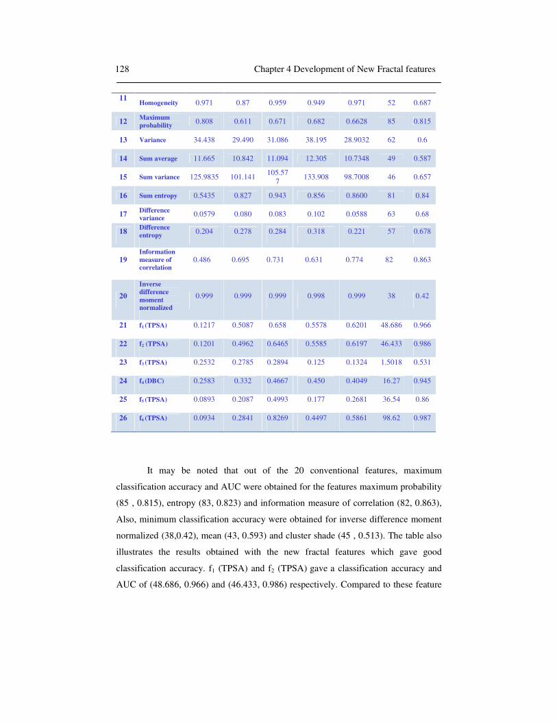
56 Chapter 4. Development of New Fractal Features
11 Homogeneity 0.971 0.87 0.959 0.949 0.971 52 0.687
12 Maximum
probability 0.808 0.611 0.671 0.682 0.6628 85 0.815
13 Variance 34.438 29.490 31.086 38.195 28.9032 62 0.6
14 Sum average 11.665 10.842 11.094 12.305 10.7348 49 0.587
15 Sum variance 125.9835 101.141 105.57
7 133.908 98.7008 46 0.657
16 Sum entropy 0.5435 0.827 0.943 0.856 0.8600 81 0.84
17 Difference
variance 0.0579 0.080 0.083 0.102 0.0588 63 0.68
18 Difference
entropy 0.204 0.278 0.284 0.318 0.221 57 0.678
19 Information
measure of
correlation 0.486 0.695 0.731 0.631 0.774 82 0.863
20
Inverse
difference
moment
normalized
0.999 0.999 0.999 0.998 0.999 38 0.42
21 f1 (TPSA) 0.1217 0.5087 0.658 0.5578 0.6201 48.686 0.966
22 f2 (TPSA) 0.1201 0.4962 0.6465 0.5585 0.6197 46.433 0.986
23 f3 (TPSA) 0.2532 0.2785 0.2894 0.125 0.1324 1.5018 0.531
24 f4 (DBC) 0.2583 0.332 0.4667 0.450 0.4049 16.27 0.945
25 f5 (TPSA) 0.0893 0.2087 0.4993 0.177 0.2681 36.54 0.86
26 f6 (TPSA) 0.0934 0.2841 0.8269 0.4497 0.5861 98.62 0.987
It may be noted that out of the 20 conventional features, maximum
classification accuracy and AUC were obtained for the features maximum probability
(85 , 0.815), entropy (83, 0.823) and information measure of correlation (82, 0.863),
Also, minimum classification accuracy were obtained for inverse difference moment
normalized (38,0.42), mean (43, 0.593) and cluster shade (45 , 0.513). The table also
illustrates the results obtained with the new fractal features which gave good
classification accuracy. f1 (TPSA) and f2 (TPSA) gave a classification accuracy and
AUC of (48.686, 0.966) and (46.433, 0.986) respectively. Compared to these feature
128 Chapter 4 Development of New Fractal features
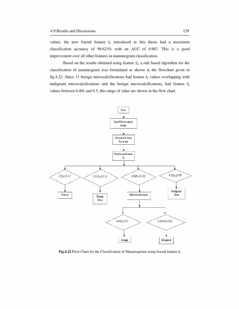
56 Chapter 4. Development of New Fractal Features
values, the new fractal feature f6 introduced in this thesis had a maximum
classification accuracy of 98.623% with an AUC of 0.987. This is a good
improvement over all other features in mammogram classification.
Based on the results obtained using feature f6, a rule based algorithm for the
classification of mammogram was formulated as shown in the flowchart given in
fig.4.22. Since 11 benign microcalcifications had feature f6 values overlapping with
malignant microcalcifications and the benign microcalcifications, had feature f6
values between 0.401 and 0.5, this range of value are shown in the flow chart.
Fig.4.22 Flow Chart for the Classification of Mammograms using fractal feature f6
4.9 Results and Discussions 129
56 Chapter 4. Development of New Fractal Features
4.10 Chapter Summary
In this chapter, a novel fractal feature derived from the TPSA method was developed
for classifying mammograms, into normal, benign and malignant masses, and benign
and malignant microcalcifications. Different fractal features mentioned by Chaudhuri
and Sarkar (Chd 1995) which were used in image segmentation, were used for
comparison of classification accuracy. Here, these fractal features are based on the
fractal dimension calculated using three methods, viz. Triangular Prism Surface Area
(TPSA) method, Differential Box Counting (DBC) method and blanket method. Of
the three methods, fractal feature 6f derived from the TPSA method gave the highest
of 98.925% classification accuracy with Malignant masses giving the highest
6f value in the range 0.7-0.986 and the least feature values of 0.001 - 0.156 were
obtained for the normal mammograms as expected. 0.209 - 0.35 is the range of
6f values obtained for the benign masses while the range of benign and malignant
microcalcifications is obtained are 0.401 - 0.5 and 0.56 - 0.62 respectively. Only for
benign and malignant microcalcification, there was not sufficient separation between
the classes.
The classification performances of these features were evaluated using
Receiver Operating Characteristics (ROC) analysis. It substantiates the obtained
results. It shows that 6f has the highest Area Under ROC curve (AUC) of 0.987 and
was able to discriminate between different classes of mammograms efficiently. Thus,
fractal feature 6f computed using TPSA method is found to be an effective and
promising way to distinguish different types of digital mammograms.
Regular screening of mammograms has been made compulsory in many
European countries for women above 40 years of age. Thus the number of
mammograms, the radiologists should evaluate will be very large. Also, majority of
the mammograms will be normal ones. As a result, radiologists are struggling hard to
differentiate between the normal mammograms and the ones with potential breast
cancer. In this scenario, radiologists are looking for a more accurate and efficient
diagnostic method for detecting cancer cells at an early stage. This study
130 Chapter 4 Development of New Fractal features

56 Chapter 4. Development of New Fractal Features
demonstrates the performance of the new technique developed for the efficient
classification of mammograms.
4.10 Chapter Summary 131