Chapter 4 – Data Transformation and Reconstruction

© 2006 Burkhard Wuensche http://www.cs.auckland.ac.nz/~burkhard Slide 1

Chapter 4 – Data Transformation and Reconstruction

4.1 Motivation4.2 Sources of Volume Data4.3 Transformation of the Independent Variable4.4 Reconstruction Filters 4.5 Transformation of the Dependent Variable4.6 References


4.1 Motivation

A multidimensional data set consist of

m independent variables representing the data domain (usually space, time).

n dependent variables defined over the domain (e.g. scalar, vector and/or tensor data).

nmL


Motivation (cont’d)Two Problems:

Data can exist in various forms (analytic functions, sampled, implicitly) but many visualization methods require a particular representation⇒Transform independent variables (e.g. interpolation,

sampling)

Data attributes contain not enough information or information isto complex ⇒Transform the dependent variable (data reduction, data

enrichment, data modification)


4.2 Sources of Volume Data

Medicine and Biology ("biomedical imaging")CT (“Computed Tomography”) ScansMRI (“Magnetic Resonance Imaging”) ScansPET (“Positron Emission Tomography”) ScansUltrasonography (ultrasonic echo-sounding)Confocal microscopy

We are predominantly interested in (time varying) volume data (m=3 or 4). Widespread in Science and Engineering, but here are just a few common examples:


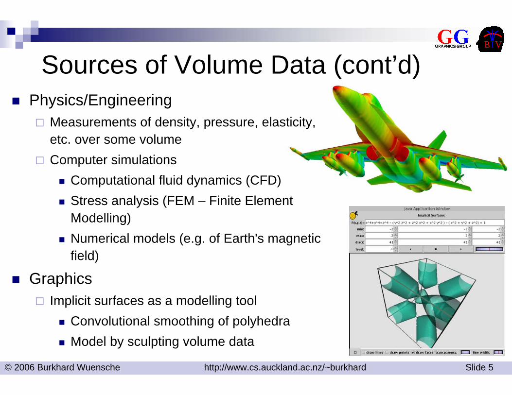
Sources of Volume Data (cont’d)Physics/Engineering

Measurements of density, pressure, elasticity, etc. over some volumeComputer simulations

Computational fluid dynamics (CFD)Stress analysis (FEM – Finite Element Modelling)Numerical models (e.g. of Earth's magnetic field)

GraphicsImplicit surfaces as a modelling tool

Convolutional smoothing of polyhedraModel by sculpting volume data


Some Volume Visualization Examples

Medicine:

MRI Data of the human brain

Biology:

Cellular structure of a sea sponge

Data source: BIRU – University of Auckland

Data source: University of Erlangen-Nürnberg

Microscience:

Molecular structure of an iron protein

Data source: Kitware Inc.


TerminologyStart with some function f(x, y, z) or f(x, y, z,t)

Called a field over R3 (or R4)We deal only in 3-D and 4-D fields, but can have arbitrary n-D fields

Have various types of fieldsScalar, i.e. f of type real

e.g. CT scan, density measurements, …Vector, i.e. f is an n-vector (commonly n = 3)

e.g. fluid velocity in a CFD simulationforce fields (magnetic, electric, gravitational)

Tensor, i.e. f is a matrixe.g. stress and strain in FEM modelling


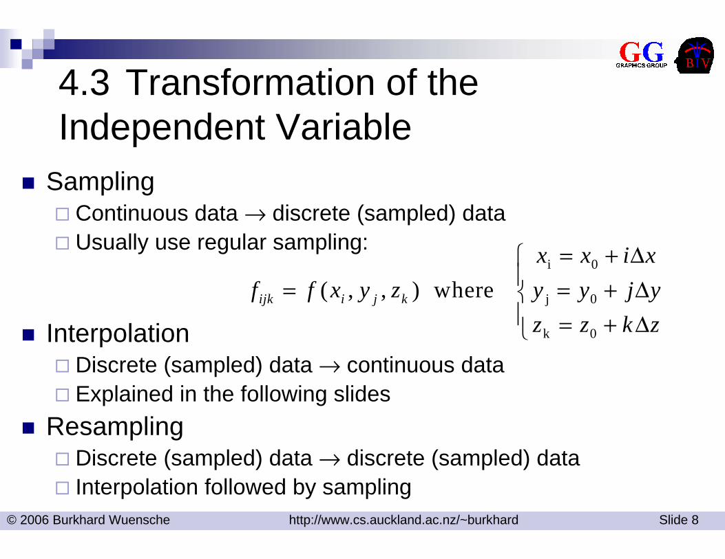
4.3 Transformation of the Independent Variable

SamplingContinuous data → discrete (sampled) dataUsually use regular sampling:

InterpolationDiscrete (sampled) data → continuous dataExplained in the following slides

ResamplingDiscrete (sampled) data → discrete (sampled) dataInterpolation followed by sampling

i 0

j 0

k 0

( , , ) where ijk i j k

x x i xf f x y z y y j y

z z k z

= + ∆⎧⎪= = + ∆⎨⎪ = + ∆⎩


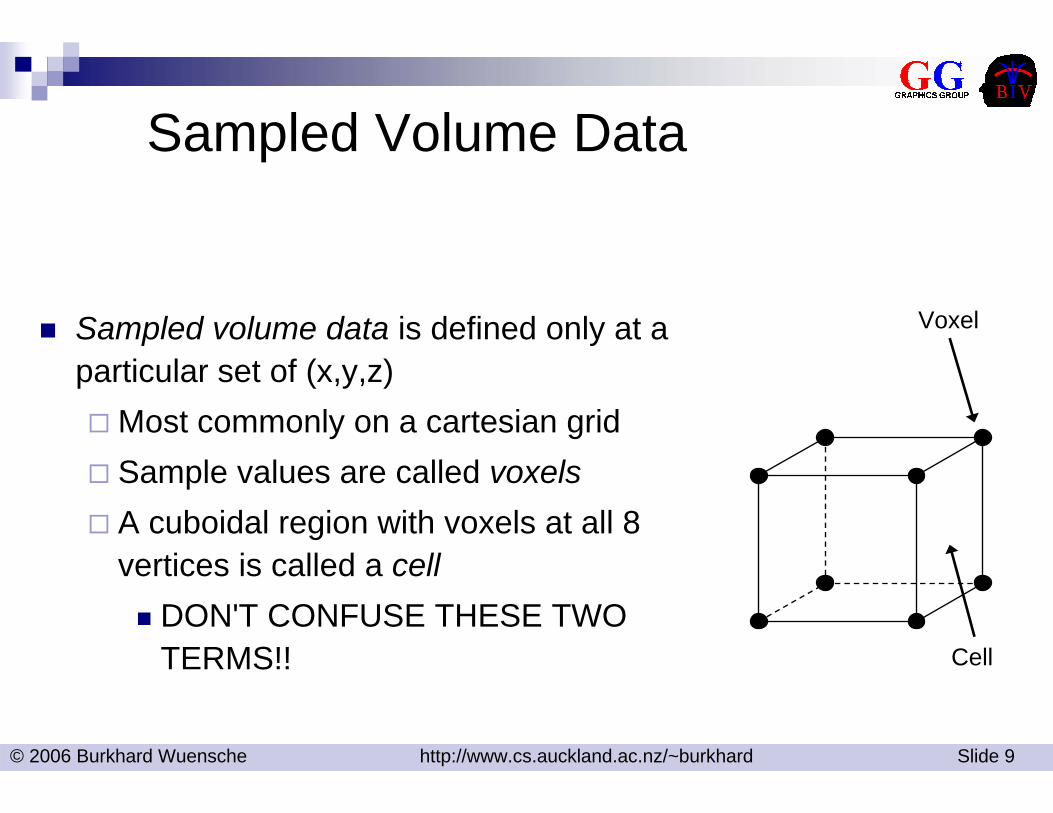
Sampled Volume Data

Sampled volume data is defined only at a particular set of (x,y,z)

Most commonly on a cartesian gridSample values are called voxelsA cuboidal region with voxels at all 8 vertices is called a cell

DON'T CONFUSE THESE TWO TERMS!! Cell

Voxel


Volumes as Fields

Important to remember that samples represent a field, i.e. a continuumProcess of defining the underlying field from a set of samples is called interpolation or reconstruction

Formally defined by convolution with a reconstruction filter (see next section)Trilinear interpolation is the most common reconstruction methodTricubic interpolation (e.g. B-spline) used for high-quality work


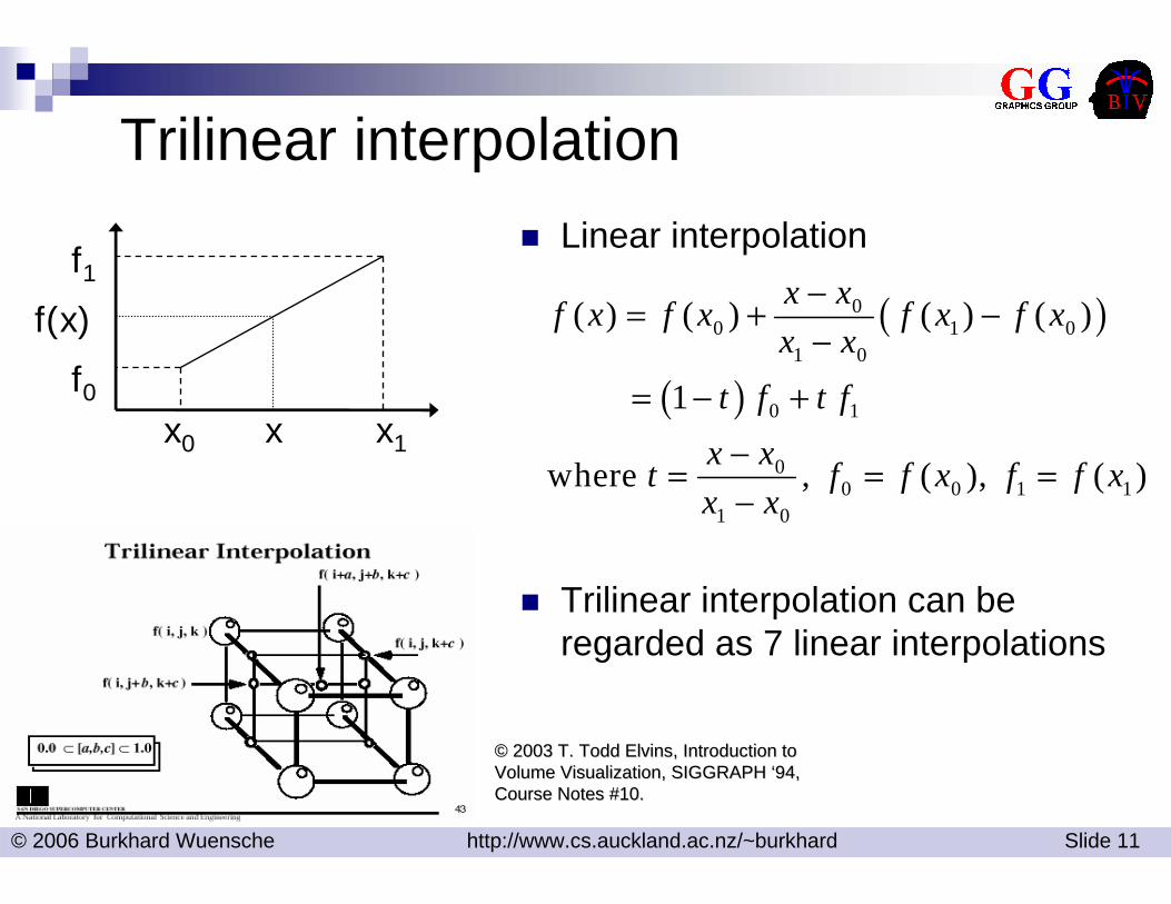
Trilinear interpolation

x0 x1xf0

f1f(x) ( )

( )

00 1 0

1 0

0 1

00 0 1 1

1 0

( ) ( ) ( ) ( )

1

where , ( ), ( )

x xf x f x f x f xx x

t f t fx xt f f x f f xx x

−= + −−

= − +−= = =−

Trilinear interpolation can be regarded as 7 linear interpolations

©© 2003 2003 T. Todd T. Todd ElvinsElvins, , Introduction to Introduction to Volume Visualization, SIGGRAPH Volume Visualization, SIGGRAPH ‘‘94, 94, Course Notes #10.Course Notes #10.

Linear interpolation


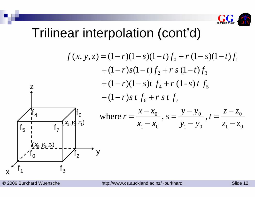
Trilinear interpolation (cont’d)

yf0 f2

x

z

f1 f3

f4 f6

f5 f7

(x0,y0,z0)

(x1,y1,z1) 01

0

01

0

01

0

76

54

32

10

, , where

)1( )-(1 )1)(1(

)1( )1()1( )1)(1( )1)(1)(1(),,(

zzzzt

yyyys

xxxxr

ftsrftsrftsrftsrftsrftsr

ftsrftsrzyxf

−−=

−−=

−−=

+−++−−+

−+−−+−−+−−−=


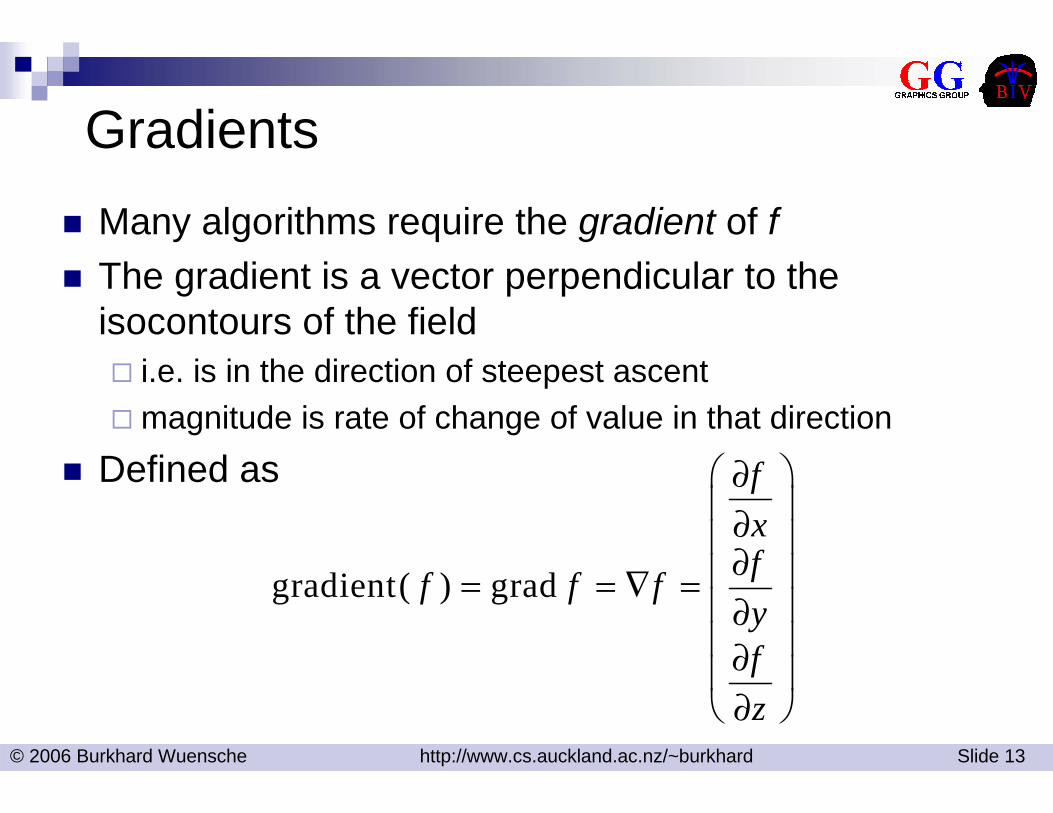
Many algorithms require the gradient of fThe gradient is a vector perpendicular to the isocontours of the field

i.e. is in the direction of steepest ascentmagnitude is rate of change of value in that direction

Defined as

Gradients

gradient( ) grad

fxff f fyfz

⎛ ⎞∂⎜ ⎟∂⎜ ⎟∂⎜ ⎟= = ∇ =⎜ ⎟∂⎜ ⎟∂⎜ ⎟

∂⎝ ⎠


Gradients (cont’d)

A trilinearly reconstructed field has discontinuous gradients at cell boundaries, so rather than computing true gradients we normally compute a smooth approximation:

Use central differences to compute gradients at voxels

Trilinearly interpolate those to get grad f (x, y, z)

( , , ) ( , , )2

( , , ) ( , , )( , , )2

( , , ) ( , , )2

f x x y z f x x y zx

f x y y z f x y y zf x y zy

f x y z z f x y z zz

⎛ ⎞+ ∆ − − ∆⎜ ⎟∆⎜ ⎟

+ ∆ − − ∆⎜ ⎟∇ = ⎜ ⎟∆⎜ ⎟

+ ∆ − − ∆⎜ ⎟⎜ ⎟∆⎝ ⎠


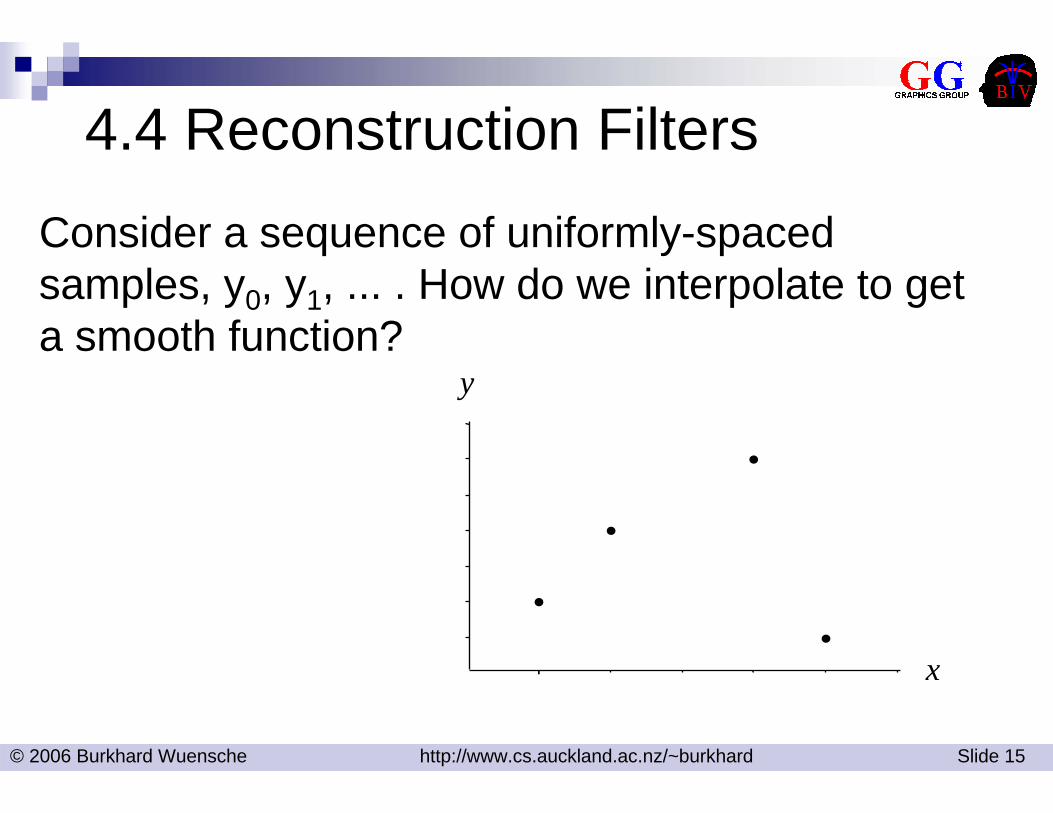
4.4 Reconstruction FiltersConsider a sequence of uniformly-spaced samples, y0, y1, ... . How do we interpolate to get a smooth function?

1 2 3 4 5 60

1

2

3

4

5

6

7

x

y


Piecewise Constant Interpolation(“Nearest Neighbour” interpolation/ box filtering)

[The unit “square pulse” function]

x1 2 3 4 5 6

0

1

2

3

4

5

6

7

x

y

( ) ( )

1 0.5 0.5where ( )

0 otherwise

iy x y U x i

xU x

= −

− ≤ ≤⎧= ⎨⎩

∑


Convolutional Smoothing

Piecewise constant is not smooth enoughCommon smoothing technique is “convolutional smoothing”

Smoothed value at any point is the average of the input functionin the vicinity of the pointUnweighted average over a fixed interval is called “running mean”Generally have a weight function or filter function, h(x)Box filtering is convolutional smoothing with square pulse, h = U

( ) ( ) ( )smoothf x f h f u h x u du∞

−∞

= ∗ = −∫


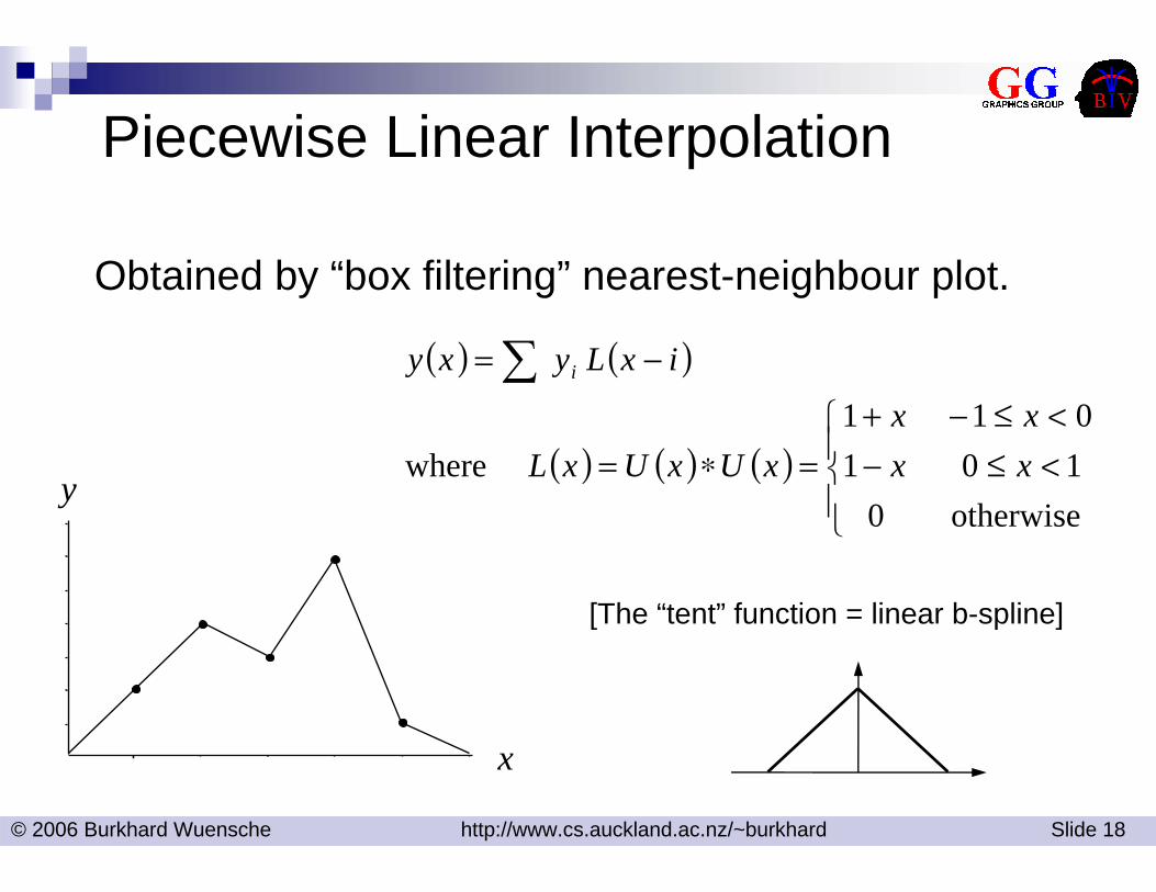
Obtained by “box filtering” nearest-neighbour plot.

Piecewise Linear Interpolation

( ) ( )

( ) ( ) ( )⎪⎩

⎪⎨

⎧<≤−<≤−+

=∗=

−= ∑

otherwise0101011

where xxxx

xUxUxL

ixLyxy i

[The “tent” function = linear b-spline]

1 2 3 4 5 60

1

2

3

4

5

6

7

x

y


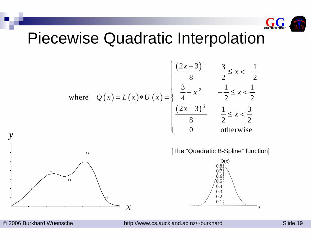
Piecewise Quadratic Interpolation

( ) ( ) ( )

( )

( )

2

2

2

2 3 3 18 2 2

3 1 1where 4 2 2

2 3 1 38 2 20 otherwise

xx

x xQ x L x U x

xx

⎧ +− ≤ < −⎪

⎪⎪ − − ≤ <⎪= ∗ = ⎨⎪ −⎪ ≤ <⎪⎪⎩

[The “Quadratic B-Spline” function]

-2 -1.5 -1 -0.5 0 0.5 1 1.5 2x0.10.20.30.40.50.60.70.8

Q(x)

1 2 3 4 5 60

1

2

3

4

5

6

7

x

y

( ) ( )iy x y Q x i= −∑


Volume ReconstructionReconstruction filters can be extended to 3D and be used to interpolate (reconstruct) sample volumes.

( ) ( ) ( )

( ) ( )

( , , )( , , )

( ) iff ( , , ) is the sample point closest to

smooth

x y z

x y z

ijk

f f h f h d

f h du du du

where x y zu u u

f f i j k

∞

−∞∞ ∞ ∞

−∞ −∞ −∞

= ∗ = −

= −

==

=

∫

∫ ∫ ∫

x u x u u

u x u

xu

u u


Volume Reconstruction (cont’d)

Separable filters can be writtenExamples are:

1 if 1( )

0 otherwisesx x

h x⎧ − <

= ⎨⎩

( , , ) ( ) ( ) ( )s s sh x y z h x h y h z=

3 2

3 2

(12 9 6 ) ( 18 12 6 ) (6 2 ) if 11( ) ( 6 ) (6 30 ) ( 12 48 ) (8 24 ) if 1 26

0 otherwises

B C x B C x B x

h x B C x B C x B C x B C x

⎧ − − + − + + + − <⎪⎪= − − + + + − − + + ≤ <⎨⎪⎪⎩

Tricubic filters: Tricubic B-Spline (B=1,C=0) Catmull-Rom Spline (B=0, C=0.5)

Trilinear filter:


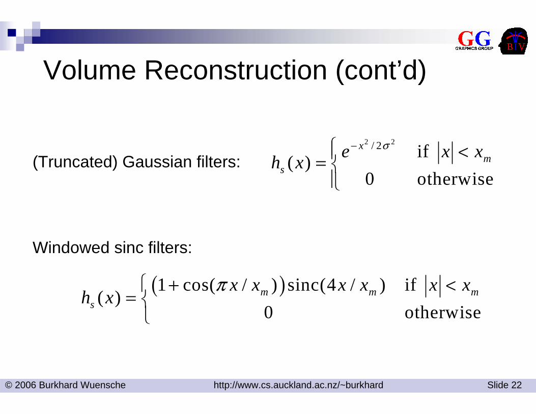
Volume Reconstruction (cont’d)

2 2/ 2 if ( )0 otherwise

xm

se x xh x

σ−⎧ <⎪= ⎨⎪⎩

Windowed sinc filters:

(Truncated) Gaussian filters:

( )1 cos( / ) sinc(4 / ) if ( )

0 otherwisem m m

sx x x x x x

h xπ⎧ + <

= ⎨⎩


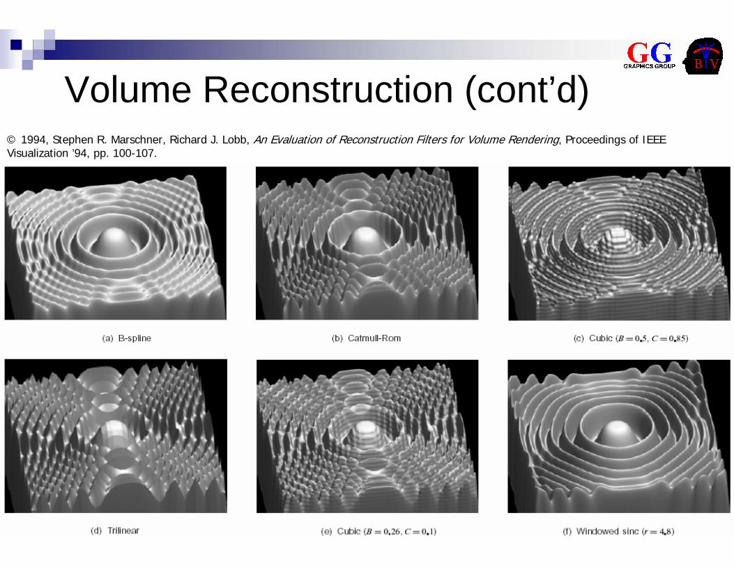
Volume Reconstruction (cont’d)© 1994, Stephen R. Marschner, Richard J. Lobb, An Evaluation of Reconstruction Filters for Volume Rendering, Proceedings of IEEE Visualization ’94, pp. 100-107.


4.5 Transformations of the Dependent Variable

We are predominantly interested in ScalarsVectorsSymmetric (2nd order) tensors

Possible Transformations of data areData reductionData modificationData expansion


Transformations for Scalar Data

Compute gradient Image Processing Algorithms

smoothing, sharpening, edge detection, …Statistical techniques for multivariate data


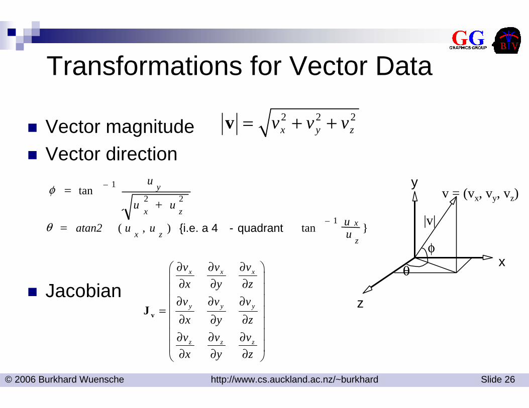
Transformations for Vector Data

Vector magnitude Vector direction

Jacobian

2 2 2x y zv v v= + +v

x

y

z

θ

φ

v = (vx, vy, vz)

|v|

φ = tan − 1 u y

u x2 + u z

2

θ = atan2 ( u x , u z ) {i.e. a 4 - quadrant tan− 1 u x

u z}

x x x

y y y

z z z

v v vx y zv v vx y zv v vx y z

∂ ∂ ∂⎛ ⎞⎜ ⎟∂ ∂ ∂⎜ ⎟⎜ ∂ ∂ ∂ ⎟

= ⎜ ⎟∂ ∂ ∂⎜ ⎟⎜ ⎟∂ ∂ ∂⎜ ⎟∂ ∂ ∂⎝ ⎠

vJ


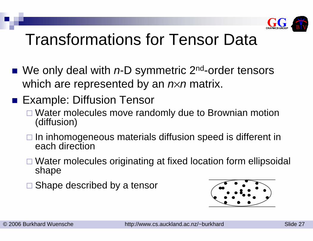
Transformations for Tensor Data

We only deal with n-D symmetric 2nd-order tensors which are represented by an n×n matrix.Example: Diffusion Tensor

Water molecules move randomly due to Brownian motion (diffusion)In inhomogeneous materials diffusion speed is different in each directionWater molecules originating at fixed location form ellipsoidal shapeShape described by a tensor


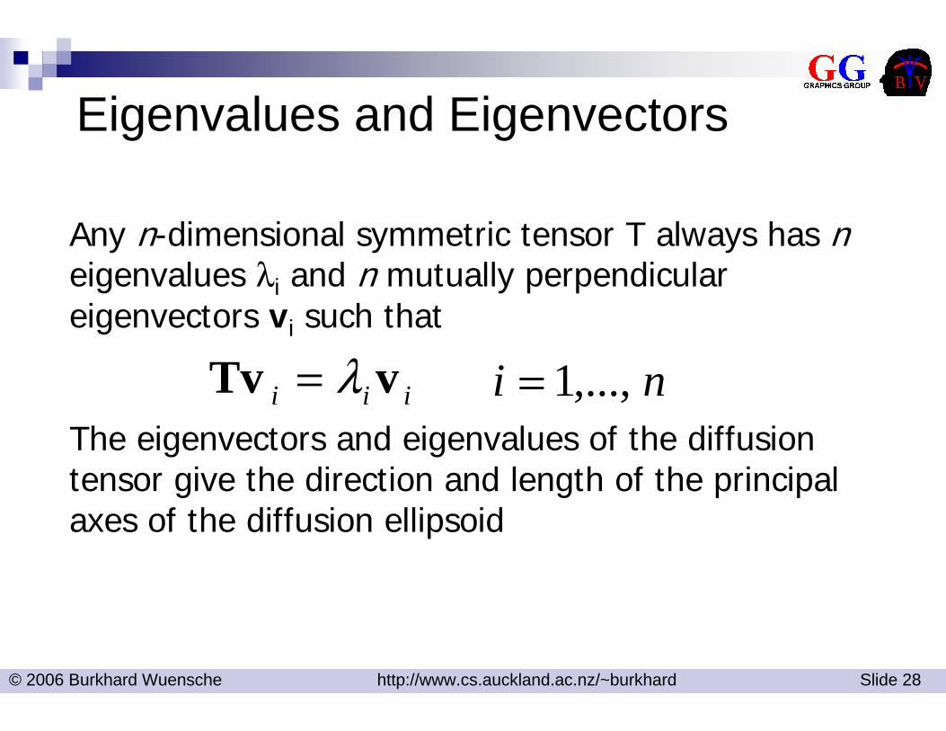
Eigenvalues and Eigenvectors

Any n-dimensional symmetric tensor T always has neigenvalues λi and n mutually perpendicular eigenvectors vi such that

The eigenvectors and eigenvalues of the diffusion tensor give the direction and length of the principal axes of the diffusion ellipsoid

iii vTv λ= ni ,...,1=


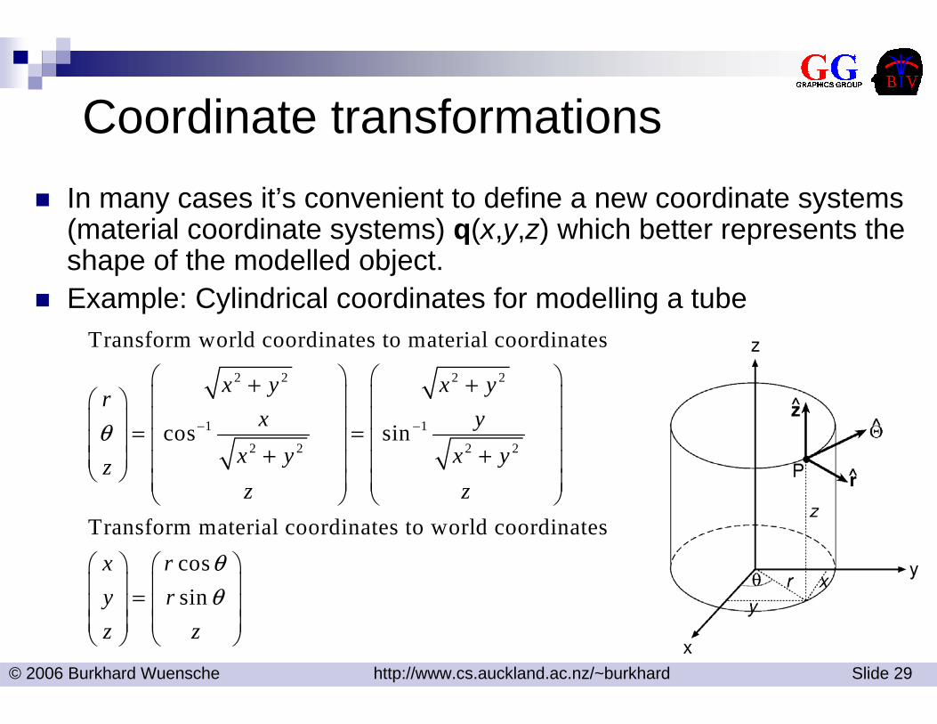
Coordinate transformationsIn many cases it’s convenient to define a new coordinate systems (material coordinate systems) q(x,y,z) which better represents the shape of the modelled object. Example: Cylindrical coordinates for modelling a tube

2 2 2 2

1 1

2 2 2 2

Transform world coordinates to material coordinates

cos sin

Transform material coordinates to world coordinates

x y x yrx y

x y x yzz z

x ryz

θ − −

⎛ ⎞ ⎛ ⎞+ +⎜ ⎟ ⎜ ⎟⎛ ⎞⎜ ⎟ ⎜ ⎟⎜ ⎟ = =⎜ ⎟ ⎜ ⎟⎜ ⎟ + +⎜ ⎟ ⎜ ⎟ ⎜ ⎟⎝ ⎠ ⎜ ⎟ ⎜ ⎟⎝ ⎠ ⎝ ⎠

⎛ ⎞⎜ ⎟ =⎜ ⎟⎜ ⎟⎝ ⎠

cossinrz

θθ

⎛ ⎞⎜ ⎟⎜ ⎟⎜ ⎟⎝ ⎠


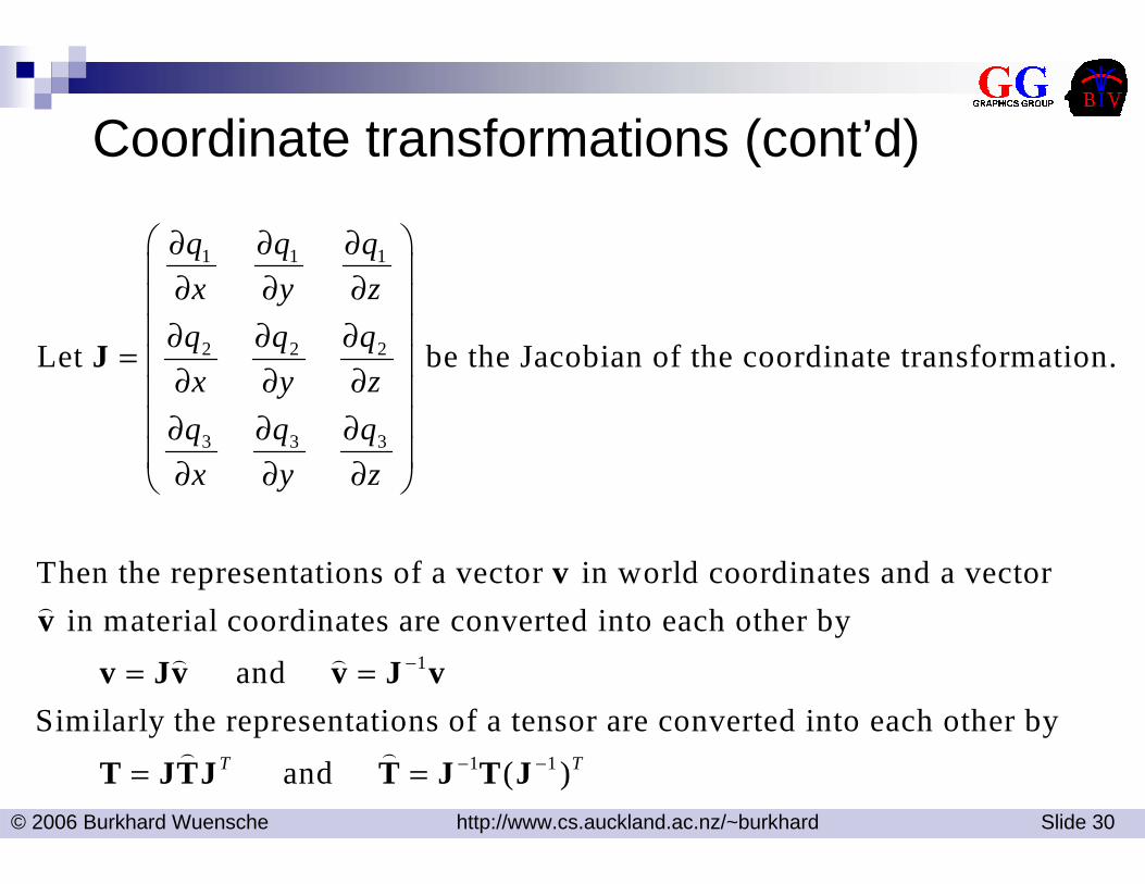
Coordinate transformations (cont’d)

1 1 1

2 2 2

3 3 3

Let be the Jacobian of the coordinate transformation.

Then the representations of a vector in world coordinates and a vector in mat

q q qx y zq q qx y zq q qx y z

⎛ ⎞∂ ∂ ∂⎜ ⎟∂ ∂ ∂⎜ ⎟⎜ ⎟∂ ∂ ∂= ⎜ ⎟∂ ∂ ∂⎜ ⎟⎜ ⎟∂ ∂ ∂⎜ ⎟∂ ∂ ∂⎝ ⎠

J

vv)

1

1 1

erial coordinates are converted into each other by and Similarly the representations of a tensor are converted into each other by

and ( )T T

−

− −

= =

= =

v Jv v J v

T JTJ T J T J

) )

) )


4.6 References

T. Todd Elvins, Introduction to Volume Visualization, SIGGRAPH 94, Course Notes #10.Stephen R. Marschner, Richard J. Lobb, An Evaluation of Reconstruction Filters for Volume Rendering, Proceedings of IEEE Visualization ’94, pp. 100-107.Burkhard Wünsche, Scientific Visualization, chapter 4, In “A Toolkit for the Visualization of Tensor Fields in Biomedical Finite Element Models”, PhD Thesis, University of Auckland, 2004.Rosenblum et al. (editors), Scientific Visualization – Advances and Challenges, Academic Press, 1994.

Documents

Chapter 4 – Data Transformation and Reconstruction