Embed Size (px)
Citation preview

43
Chapter 4- Control Delay Analysis at an Intersection Intersection control delay
The delay encountered by a traveler at a signalized intersection constitutes the
larger part of his and her travel time on an arterial link. Hence, estimating the control
delay plays a very important part of the travel time estimation of an arterial link. The
methodology used in estimating the control delay is a combination of the shockwave
algorithm developed earlier by Hobeika et.al, and adjusted algorithms of HCM2000
that recommends certain methods for computing the delays at a signalized
intersection.
The control delay experienced by the observed group has three main components:
the uniform stop delay (d1), the over-saturation delay (d2), and the stopped delay
caused by the initial queue accumulated behind the intersection from previous cycles
(d4):
delaystoppeddelaytionoversaturadelayuniformdelaycontrol −++= ___ .
However, in order to compute the stopped delay of the observed vehicle group (d4)
which is caused by the initial queue, the initial queue clearance time (d3) needs to be
determined first. d4 is the average stopped delay of the observed group during time
d3.that certain vehicles in the observed group while the initial queue is being cleared
(during d3). Therefore, the intersection control delay in our methodology is computed
as follows:
421_ ddddelaycontrol ++=

44
4.1 Definition of New Variables Used in Chapter 4
d1: Uniform stop delay of the observed group when dissipating the intersection;
d2: Over-saturation delay of the observed group when dissipating the intersection.
d3: Initial delay encountered by the first vehicle of the observed group to reach the
intersection caused by the queue built up from previous cycles.
d4: Average stopped delay of the observed vehicle group caused by the initial
queue, or during time d3. (See section 4.3.4 for further explanation)
h1: Original uniform headway of the observed group. (sec/veh);
h2: Intersection departure headway.( sec/veh); usually considered to be 2
secs/veh= 3600/1800
h3: Queue departure headway (sec/veh);
:mQ Number of vehicles from the observed group that joins the queue during the
red phase,(veh);
qt : The time it takes the queue from the observed group to develop and to
dissipate during a cycle length, (sec)
S1: Average arrival speed of the observed vehicle group at the detector, (mph)
S2: Moving speed of the queue at the intersection (mph);
The following relationships and assumptions are adopted:
a) The control delay is the average control delay of all the vehicles in the
observed group.
b) The headway distribution and the speed of the observed group will change due
to the initial queue. This assumption will be described later on.
45
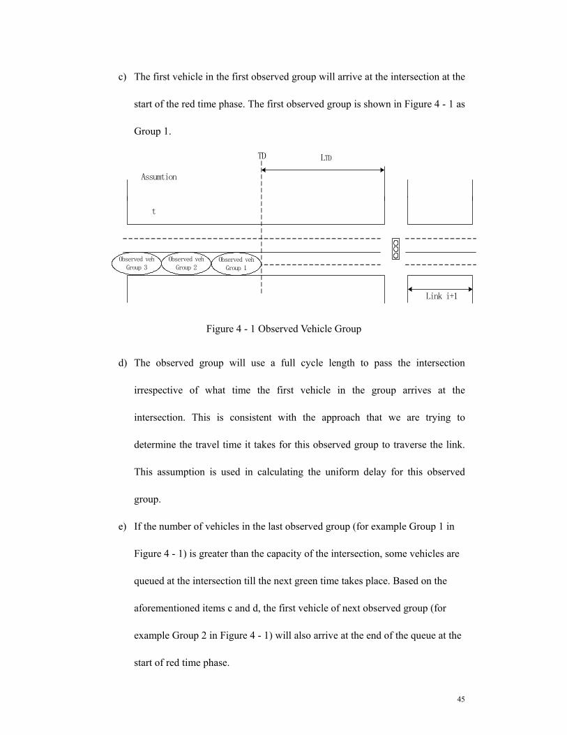
c) The first vehicle in the first observed group will arrive at the intersection at the
start of the red time phase. The first observed group is shown in Figure 4 - 1 as
Group 1.
Link i+1
LTDTD
Observed vehGroup 1
Observed vehGroup 2
Observed vehGroup 3
Assumtion
t
Figure 4 - 1 Observed Vehicle Group
d) The observed group will use a full cycle length to pass the intersection
irrespective of what time the first vehicle in the group arrives at the
intersection. This is consistent with the approach that we are trying to
determine the travel time it takes for this observed group to traverse the link.
This assumption is used in calculating the uniform delay for this observed
group.
e) If the number of vehicles in the last observed group (for example Group 1 in
Figure 4 - 1) is greater than the capacity of the intersection, some vehicles are
queued at the intersection till the next green time takes place. Based on the
aforementioned items c and d, the first vehicle of next observed group (for
example Group 2 in Figure 4 - 1) will also arrive at the end of the queue at the
start of red time phase.
46
HCM2000 uses a relatively large observed time period such as 15 minutes, or half
an hour to estimate the control delay at a signalized intersection. But in our case, we
need to update the travel time of the observed vehicle group for each one or two
minutes. Hence, we had to adjust the equations for computing the control delay in
HCM2000 in order to apply to our cases.
4.2 Computing the Initial Delay of the First Vehicle in the Observed Group(d3)
In HCM2000, the initial delay d3 is computed as follows:
CTtuQ
d b )1(18003
+= ……………………………………………………………………(Eq 4 - 1)
Where
bQ = Initial queue at the start of period T(veh),
C= capacity(v/h);
T=duration of analysis period(h);
t= duration of unmet demand in T(h), and
u= delay parameter.
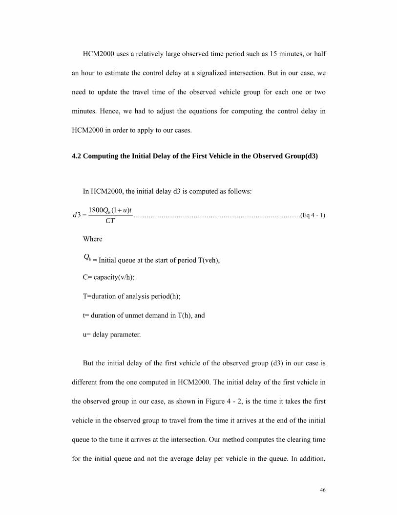
But the initial delay of the first vehicle of the observed group (d3) in our case is
different from the one computed in HCM2000. The initial delay of the first vehicle in
the observed group in our case, as shown in Figure 4 - 2, is the time it takes the first
vehicle in the observed group to travel from the time it arrives at the end of the initial
queue to the time it arrives at the intersection. Our method computes the clearing time
for the initial queue and not the average delay per vehicle in the queue. In addition,
47
after the first vehicle in the observed group arrives at the intersection, the character of
the observed group will change during the initial delay time. Hence, it will affect the
uniform stop delay, as well as the over-saturation delay, which will be discussed later
on.
Loop detector Initialqueue
Observed vehicles group
Figure 4 - 2 Initial Delay
Different from HCM2000, the adopted approach uses the shockwave method to
estimate the initial delay of the first vehicle in the observed vehicle group and the
initial queue.
If there is no blackout taking place on the loop detector which means that the
traffic data observed by the loop detector is reliable, the shockwave method is used to
estimate the initial queue length and then estimate the initial delay. The shockwave
method utilized here is the same one used in the freeway case.
(Please refer to those notes for complete description of the shockwave method).
There are three cases for estimating the initial delay: a building queue case, a
dissipation queue case and no change of queue case.
Step 1:
qtdu kk
CVW−−
= , for the building queue case where V>C ;……………………(Eq 4 - 2)

48
tdqd kk
VCW−−
= , for the dissipation case where V<C; …………………………… (Eq 4 - 3)
0=W , for no change in queue case where V=C; ………….………..... (Eq 4 - 4)
Where
tdk : is the vehicular density obtained from the detector;
qk : is the jam density.
The queuing rate QR (veh/h) is:
( )tCV du kWdtdnQR ×−−== ;…………………………………………………...….(Eq 4 - 5)
Step 2:
The number of vehicles in queue which is built during the observed cycle length t
will be:
CLQRQm ×= ………………………….…………………………………...……………..(Eq 4 - 6)
The process is repeated for every interval and the total number of vehicles in
queue is estimated using the following expression:
),0max(1∑=
=t
mmt QQ …………………………………………………….………………...(Eq 4 - 7)
tQ is the initial queue for next cycle length which is also the queue at the end of
cycle t. Thus, if we want to estimate the initial delay for cycle length t, we should
consider the queue at the end of last cycle length which is 1−tQ .
If gD
Q
s
t <−1 , the initial delay is s
t
DQ 1− +red ( sD is the departure saturation flow in green time
veh/h/ln)
Else

49
If gD
Q
s
t 21 <− , the initial delay is timeredD
Q
s
t _21 ×+− ;(because it should wait for
another green time to dissipate the initial queue vehicle for the incoming group of
vehicles in time t)
Else
If gD
Q
s
t 31 <− , the initial delay is timeredD
Q
s
t _31 ×+− ;
……
Thus, we came out with the following equation to estimate the initial delay.
When gnD
Qgn
s
t ×≤≤×− −1)1( , ……………………………………………………..(Eq 4 - 8)
Therefore, d3 = timerednD
Q
s
t _)(1 ×+− …………………………………………………(Eq 4 - 9)
Step 3:
After we conducted a calibration method using CORSIM, the average length of
the vehicle plus the average headway in queue is considered to be 19ft.
Hence the queue length, tQQL ×= 19 ,
Where
tQ is number of the vehicles in the queue at the end of current time interval.
The average speed of vehicles in the observed group is:
Speed= Volume/Density=tdkNV /
…………………………………..…………..(Eq 4 - 10)
50
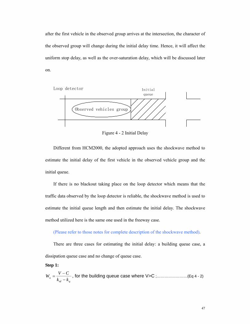
4.3 Computing Uniform Stop Delay, (d1)
Uniform delay is caused by cyclic interruption of service caused by the red phase
at a signalized intersection. Part of the observed group of vehicles will stop and queue
because of the red light, if there is no initial queue. The area of the yellow triangle in
Figure 4 - 3 is the total uniform delay time for each cycle length.
Figure 4 - 3 Uniform and Over-saturation Delay 22
A diagram of the yellow triangle is shown in Figure 4 - 4. It shows the build up of
the queue during the red phase to Qmax, and then its dissipation during part or whole
of the green time phase.
Red time Green time
Q size(veh)
h1
h3
Qmax
tq Figure 4 - 4 Uniform Delay

51
If there is no initial queue, the uniform delay in HCM2000 is computed as
follows, based in Figure 4 - 4:
Average uniform delay )),1(min(1(
)1(2
),min(5.0
1
2
max
CLg
CVCLgCL
CLCVtQ
d q
×−
−×=
×
××= …….(Eq 4 - 11)
For a detailed derivation of this equation refer to Appendix A.
We have three main concerns in adopting Equation 4 of HCM2000 in calculating
the uniform delay of the observed group. Each of the concerns is discussed separately
below:
4.3.1 The Denominator in Equation 2-11
The denominator in Equation 4 reflects the volume approaching the intersection
or the capacity of the intersection in calculating the uniform delay. When the
volume is greater than the capacity, it uses capacity as the volume to estimate the total
uniform delay. In our algorithm, we agree to use the same numerator which is
qtQ ×× max5.0 in equation 4, but since we are considering the average uniform stop
delay for all vehicles in the observed group, the total stop delay should be divided by
the total number of vehicles in the observed group instead of the value
of CLCV ×),min( . Hence, the new average uniform stop delay is computed as
follows:
Average uniform delayCLV
tQd q
×
××= max5.0
1 …………………………………………(Eq 4 - 12)

52
Queue Departure Rate h3
HCM2000 assumes that in every second, there will be 1
1h
vehicles added to the
queue and 2
1h
vehicles will be dissipated from the queue. Hence, the queue
departure rate is 1
12
1hh
− (veh/sec) which is 3
1h
. Therefore, h3 is 2121
hhhh
−×
(sec/veh). This calculation of h3 works well when there is no initial queue at the
intersection, but it may not work well when there is an initial queue at the intersection.
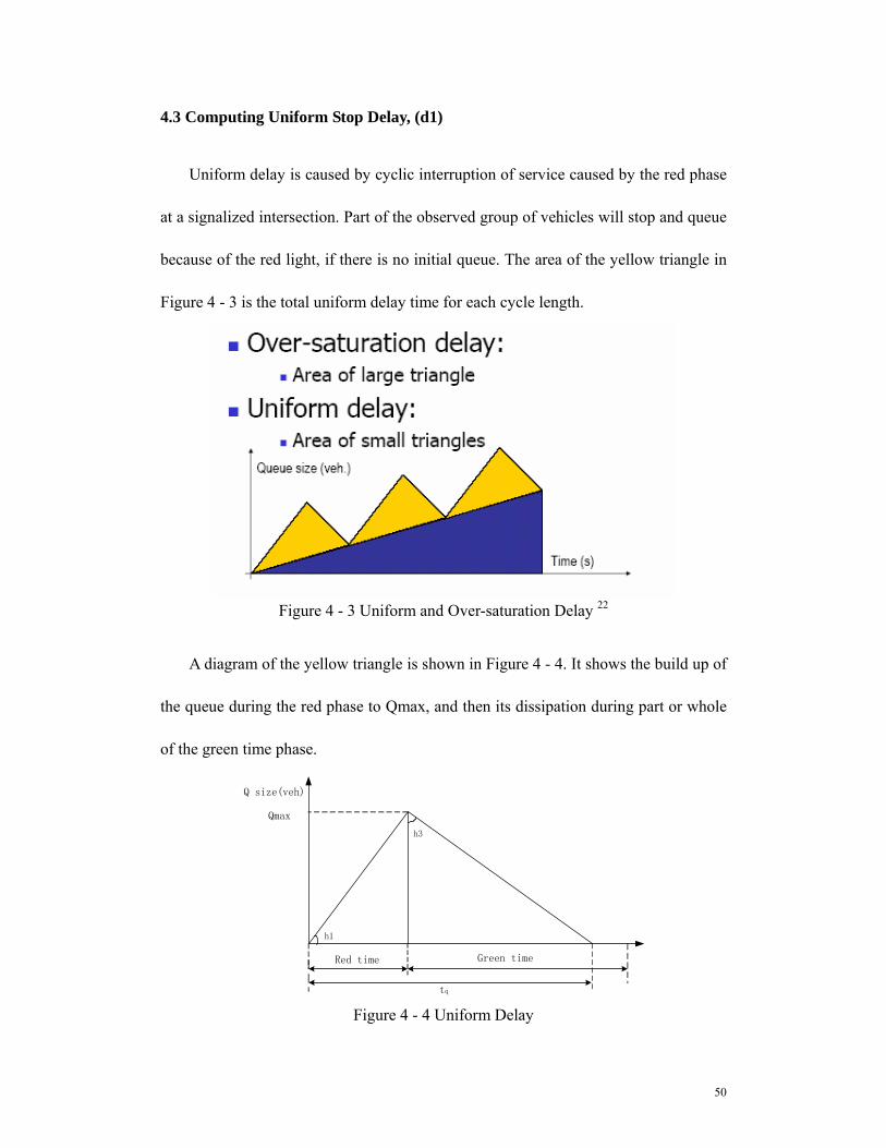
To illustrate, consider the problem shown in Figure 4 - 5, where h1 is assumed to be 5
sec/veh, and h2 to be 2 sec/veh. After 10 seconds of green time, vehicle 10 will arrive
at the queue according to HCM2000, but in actually it doesn’t, because the queue is
moving forward. Vehicle 10 only arrives at a location L where it may starts to reduce
its speed in order to enter into the queue. Hence, it doesn’t belong to the queue size
yet, because vehicle 9 has moved downstream a little bit. The distance between
vehicle 10 and vehicle 9 is greater than queue distance. This example shows that the
value of h3 is under-estimated in HCM2000 when there is a long initial queue.
53
Link i+1
Iq
LTD
12345691020
Qmax
Observed vehicle group
78
5sec
L
LIq
Link i+1
LTD
12345691020
Observed vehicle group
78
L
Q
Greater than queueheadway and spacing
At time t+10
At time t
5sec
Figure 4 - 5 Moving Queue
To refigure the new queue dissipating rate (h3) during the green time with an
initial queue, the following steps are adopted:
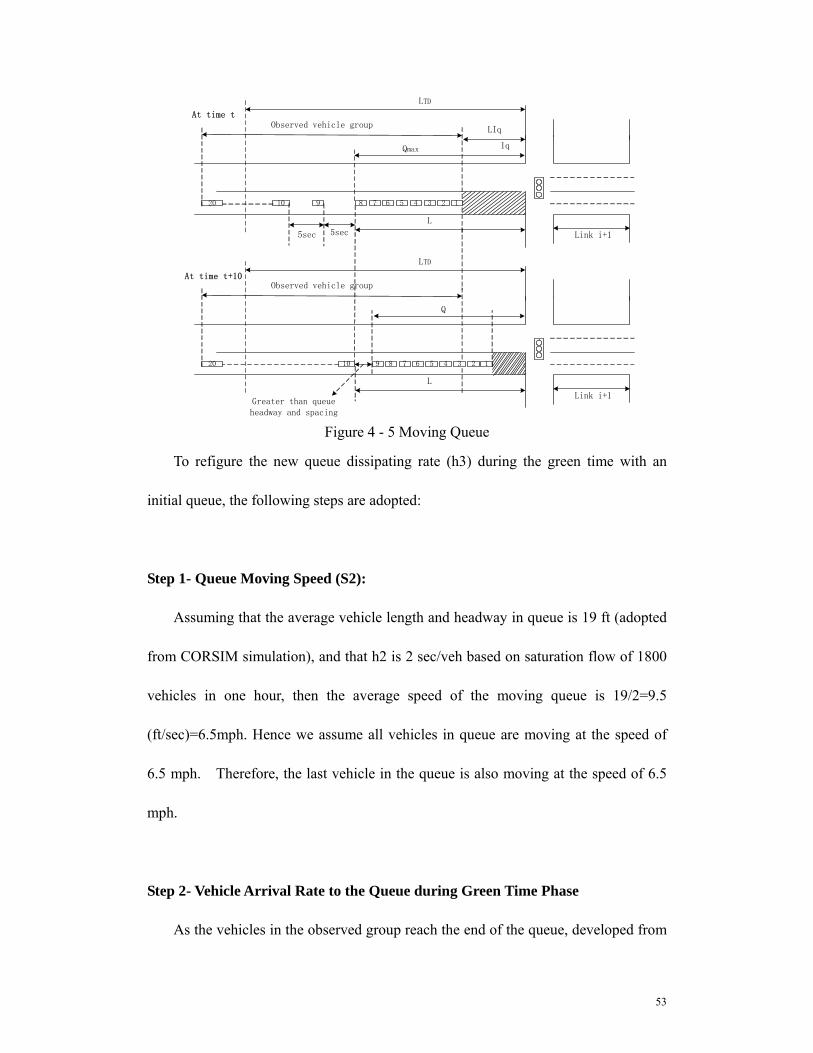
Step 1- Queue Moving Speed (S2):
Assuming that the average vehicle length and headway in queue is 19 ft (adopted
from CORSIM simulation), and that h2 is 2 sec/veh based on saturation flow of 1800
vehicles in one hour, then the average speed of the moving queue is 19/2=9.5
(ft/sec)=6.5mph. Hence we assume all vehicles in queue are moving at the speed of
6.5 mph. Therefore, the last vehicle in the queue is also moving at the speed of 6.5
mph.
Step 2- Vehicle Arrival Rate to the Queue during Green Time Phase
As the vehicles in the observed group reach the end of the queue, developed from

54
the red time of the previous cycle length, they will change their speeds and
correspondingly their headways in order to enter the queue. When the queue is
moving, the arrival rate of the observed group to enter the queue will change as stated
in section 2.3.2. The following discussion is centered on how to determine the
arrival rate of the observed group to the queue during the green time phase. Assume
that a vehicle in the observed group will join the moving queue in t seconds. Let
vehicle n be the last vehicle in the observed group that arrives at the queue in the red
time phase of the current cycle length. After t seconds, the next vehicle n+1 will join
the queue. To compute the value of t or headway, the following relationships and
assumptions are adopted:
A) Only two speeds and consequently two headways are adopted to occur in
this movement of the observed group of vehicles. We already have shown
that the saturated departure headway (h2) in green time at the intersection
is 2sec/veh and the queue moving speed is 6.5 mph (S2). The incoming
speed (S1) of observed group is obtained from the detector, and so its
uniform headway (h1).
B) The difference in the distance traveled by the nth vehicle and its follower
(n+1) in time t during the green time phase is computed based on the
difference in speeds. The distance between vehicle n and (n+1) before n
enters the queue is S1*h1. At time t0, vehicle n enters into the queue. At
time t0+t, vehicle n+1 arrives at the end of queue behind vehicle n with
19 ft headway. Hence, in time interval t, the distance change between

55
vehicle n and n+1 is (S1*h1-19).
Let the difference in distance traveled be represented as tSS ×− )21( .
Hence,
)21(1911
1911)21(
SShSt
hStSS
−−×
=⇒
−×=×−……………………………………...…..……..(Eq 4 - 13)
And the arrival rate to the queue is t (sec/veh) which means one new vehicle will
join the moving queue in every t seconds.
Step 3- Actual Queue Dissipating Rate (h3)
Now we know that the new arrival rate to the queue is t ( sec/veh). Hence, t1
vehicles will come to the queue as well as 2
1h
vehicles will dissipate from the queue
in every second. Hence, the actual dissipating rate of the queue in vehicle per second
is th1
21− ( veh/sec) which is
31h
. Therefore, the new h3 (different from HCM2000)
is 22
htht
−× (sec/veh). It is represented by the angle shown in Figure 4-6.
Red time Green time
Q size(veh)
h1
New h3
Qmax
tq
Figure 4 - 6 Queue Dissipating Rate (h3)
From Figure 4 - 6, we can compute the tq based on the new angle of h3 and the

56
Qmax.
Step 4- Computing the Uniform Delay with no Initial Queue
When there is no initial queue, the average uniform stop delay for the observed
group is computed based on the above discussions, as follows:
GroupObservedinvehiclesTotaltQ
d q
____5.0
1 max ××= ………………………….………(Eq 4 - 14)
Where
1)(_
max hrtimeredQ =
rQhtq +×= max3
Total vehicles in the observed group CLV ×=
4.3.2 Computing the Uniform Stopped Delay with an Initial Queue
The headway and speed of the observed group will also change when they
arrive at the intersection if there is an initial queue. For example, at time t in Figure 4 -
7, the first vehicle of the observed group arrives at the end of the initial queue as
explained earlier and reduces its speed and consequently joins the queue at the
intersection. When the green phase starts, it will take d3 seconds to dissipate the
initial queue till vehicle 1 in the observed group arrives at the intersection. As shown
in Figure 4 - 8, vehicle 1 arrives at the intersection, and other n vehicles following it
will join the queue during the time interval of d3. But there are some vehicles in the
observed group that are still moving with original h1 headway which is 5sec/veh.

57
Link i+1
Lq
Link i
LTDTDTime at t
6 5 4 3 2 15sec 5sec 5sec 5sec 5sec
20
Observed group,20 veh
Figure 4 - 7 At time t
Link i+1Link i
LTDTDTime at t+d3 sec
n 4 3 2 15sec
20
Observed group,20 veh
Figure 4 - 8 at time t+d3
The queue in the observed group will attempt to leave the intersection in the
remaining green time period g1=(g-d3) after d3 seconds has expired to dissipate the
initial queue. Figure 4 - 9 shows the queue build up and dissipation for the observed
group during a full cycle length period. The area under the curve in Figure 4-9
represents the uniform stopped delay with an initial queue, which is different from the
area under the curve in Figure 4-6 when there is no initial queue. It is immediately
realized that g1 is dependent
on d3, which is influenced by the size of the initial queue. So, the following
relationships are established to encompass the various initial queue size situations.
When d3 is smaller than a cycle length:
2_1 hqueueInitialg ×= , where h2 is 2 sec/veh.

58
1_2 gtimegreeng −= ;
When; cycle length≤d3≤2*cycle length
timegreenhqueueInitialg _2_1 −×=
1_2 gtimegreeng −=
When 2*cycle length≤d3≤3*cycle length
timegreenhqueueInitialg _22_1 ×−×=
1_2 gtimegreeng −=
g1 r g2
CL
Queue Size
Figure 4 - 9 Uniform Stopped Delay
Therefore, it is necessary to estimate the new characteristics of the observed
group to compute the uniform stopped delay of the queued vehicles in the observed
group while attempting to dissipate through the intersection. The uniform stopped
delay will vary, as stated above with the size of the initial queue, and the volume of
the observed group.
We have four cases that describe these variations in queue size and volume in
determining the stopped delay. They are:
Case 1- where the volume of the observed group is smaller than the intersection

59
capacity and where d3 is smaller than the cycle length
Case 2- where the volume of the observed group is greater than the capacity and d3 is
smaller than a cycle length
Case 3- where d3 is greater than a Cycle Length
Case 4- is a special case where vehicle 1 in the observed group does not reach the
initial queue at the beginning of the red phase.
Case 1- the volume of the observed group is smaller than the intersection
capacity and d3 is smaller than the cycle length
Figure 4-10 shows the development of the queue size in vehicles over time at a
signalized intersection. As we have stated earlier the queue is made up of two
components: 1) the initial queue from previous cycles, and 2) the queue of the
observed group in this time interval or cycle length.
Let Iq be the initial queue at the intersection from previous cycles. As shown in
Figure 4-10 the queue will grow during the red phase to include the incoming vehicles
from the observed group. At the end of the red time, the queue is now Iq +m. It will
take a time of g1 from the green phase to clear the initial queue. At this time the queue
size is k because some additional vehicles have joined the queue from the observed
group. The queue will still decrease till the end of the green phase (g1+g2) and now
reaches the level of L. The queue will start to build up again during the red phase.
However, we need to separate the status of the vehicles in the observed group to the
status of what is happening at the intersection as a whole. In that regard, we separated
the queue development into a) the queue of the observed group and b) the queue at the

60
intersection. The queue of the observed group, which is our main interest, now
increases for a short period of time (t4-t3) to i, as shown in Figure 4-10, and then
remains constant during the red phase, and then dissipates again during the next green
phase using a time (t6-t5).
After t3 in the Figure 4-10, the broken upward line represents the queue at the
intersection which composes of current queued vehicles and the anticipated queues
from the next observed group. The dark line in Figure 4-10 represents the queue size
of the current observed group. The area under this line, areas A, B, and C will
determine the uniform stopped delay of the observed group.
Red timeg1 g2 Red time
g1
d3
m+Iq
h2
Cycle length for observed group
Q sizein veh
t2
Area of A Area of B
t3 t4
t6
t7
Iq
Time at t1Figure 2-12
t1
Queue at the intersection
Figure 2-13
Figure 1
10sec
m+Iq-10/h3
h3
h1
Figure 2-14k Figure 2-15
L
t5
Figure 2-16
i
Initialqueue(Iq)
Areaof C
Queue build up by nextobserved group
Queue sizeof observed group
t0
Cycle length 100sec
Figure 4 - 10 Uniform Stopped Delay
To better illustrate the progression of the queue development in Figure 4-10, the
following Figures are provided by key time periods.
At time t0
Figure 4 - 11 shows the beginning situation at time t0, where the first vehicle in
the group arrives at the end of the initial queue (Iq) at the start of the red phase.

61
Link i+1
Lq
LTDTD
Observed veh Group at t
Beginning of red time)
With originial headway h1
Stop
Figure 4 - 11 at time t0
At time t1
During the red time phase from t0 to t1, the queue size at the intersection will
increase at a queue building rate of h1 (as explained earlier), reaching the value of m.
Hence, m is equal to 1
_h
timered . Therefore, at the end of red time phase, the queue
size at the intersection is Iqm + as shown in Figure 4-10.
Link i+1
Lq
LTDTDFigure 2
12345691020
Q=m=red/h1
Observed vehicle group
78
5sec
Figure 4 - 12 Time t1
From t1 to t2
During the green time phase g1 from time t1 to t2, the queue size at intersection
will be reduced at the rate of h3 to the level k. The estimation of h3 is stated earlier in

62
section 2.3.2.
Link i+1
LTD
12345691020
Observed vehicle group
78
5sec
Time from t1 to t2
11
m+Iq-10/h3
Queue of observed group
Vehicle 10 does not reach the queue because queue is moving even though the moving speed is very small
Figure 4 - 13 Time t1 to t2
At time t2
At time t2, the first vehicle of the observed group arrives at the intersection as
shown in Figure 4-14. Let k be the queue size at the intersection at time t2. From
Figure 4-10, k is derived to be equal to 31
hgIqmk −+= . At time t2, all the vehicles in
the initial queue have cleared the intersection, because d3 is less than the cycle length.
Meanwhile, all vehicles in the queue at the intersection at time t2 are the vehicles of
the observed group. Hence, k is also equal to the queue of the observed group.
Link i+1
LTD
12345691020
Observed vehicle group
78
5sec
Time at t2,
k
k
Queue of observed group
K+1
Figure 4 - 14 Time t2

63
At time t3
The red time phase starts again at time t3. As shown in Figure 4-10, t3 is also the
time for the last vehicle in this observed group to attempt to arrive at the intersection
(t3-t0=100seconds=the assumed cycle length). Figure 4 - 15 shows the distribution of
the vehicles in the current observed group at this time. As shown in Figure 4-10, from
time t2 to t3 which represents the remaining green time g2, some vehicles in the
observed group have already cleared the intersection, while some others have joined
the queue, and some others are still attempting to join the queue since the approaching
volume V is smaller than the capacity. For instance, as shown in Figure 4 - 15, vehicle
20, which is the last vehicle in the observed group, doesn’t join the stopped vehicles
at the intersection till t4 in the red time phase. The value of L in Figure 4 - 15 and in
Figure 4-10 represents the number of vehicles in the observed group that are part of
the stopped vehicles at the intersection at the start of the red phase.
Based on Figure 4-10, L is computed as follows:
321
hggIqmL +
−+= ……………………………………………………….(Eq 4 - 15)
And
When L>0
The area of A, which represents part of the uniform stopped delay, is a trapezoid
which can be calculated as follows:
The area of A is 2)(5.0 gLka ×+×= ….………………………………….(Eq 4 - 16)
When L=0, the area of A is a triangle,

64
235.035.0 khhkka ××=×××= ……………………………………(Eq 4 - 17)
Link i+1
LTD
20
Observed vehicle group
T i m e a t t 3 ,
Queue ofobserved group
5sec
LIq
L vehicles
Figure 4 - 15 Time t3
From t3 to t5
The time form t3 to t5 represents the red time phase, as shown in Figure 4-10.
During this time some of the remaining vehicles in the observed group that did not
already join the queue are still attempting to join the stopped queue at an arrival rate
of h1. From time t4 to t5, all the remaining vehicles in the observed group would have
joined the stopped queue as shown in Figure 4-16. The number of vehicles in this
queue would remain constant for the rest of the red time phase. The number of
vehicles in queue from t4 to t5 is equal to the number of vehicles in the observed
group which can not dissipate the intersection during time t2 to t3 (g2). The
dissipating rate of the observed group in the queue from time t2 is h2 which is always
2 sec/veh. Hence, the number of vehicles in queue from t4 to t5, represented as (i), is
computed by subtracting the number of vehicles in the observed group (V.CL) from
the number of vehicles that already left the intersection (g2/h2):
22
hgCLVi −×= ……………………………………………………………………..(Eq 4 - 18)
The vehicles that would be still approaching the queue from this group during this
period are the difference between the two sizes of queue i and L as shown in Figure

65
4-10.
1)(34 hLitt ×−=−
Therefore, the area B under the curve, which represents the stopped delay can now be
calculated as follows:
))34(()34()(5.0 ttredtimeittiLb −−×+−×+×= ………………………(Eq 4 - 19)
Link i+1
LTD
20
Observed vehicle group
Time at t4 and t5,
Queue ofobserved group
LIq
i vehicles
Figure 4 - 16 Time t3 to t5
From t5 to t6
The time from t5 to t6 represents part of the green time phase for the next cycle
length. The number of vehicles i in the observed group would now dissipate at an h2
rate Since the volume of the observed group is smaller than the capacity in this case,
all vehicles in the queue can dissipate in time g1.
From Figure 4-10, the C area under the curve that represents the uniform stopped
delay is computed as follows:
225.025.0 ihhiic ××=×××= ..............................................................................(Eq 4 - 20)
Hence, the average stopped delay of case 1 is computed by adding areas A,B, and C
and divide by the number of vehicles in the observed group (VxCL):

66
CLV
cbad×++
=1
Case 2, Volume of the observed group is greater than the intersection capacity
and d3 is smaller than the cycle length
This case 2 is very similar to case 1 except that intersection capacity is now used
instead of the observed volume in calculating the dissipating volume at the
intersection. This logically would result that all vehicles in the observed group can
dissipate the intersection during the whole green time, and that the queue at the start
of the next cycle is the same as the starting initial queue. Therefore, from Figure 4-17
the value of i in case 2 is equal to the initial queue size (Iq) which is equal to
21
22
hg
hgCLC =−×
Red timeg1 g2 Red time
g1
d3
m+Iq
r+g1+g2=100 sec
h2
Cycle length for observed group
Q sizein veh
t2
Area of A Area of B
t3 t4
t6
t7
t1
Queue at the intersection
10sec
m+Iq-10/h3
h3
k
L
t5
Initialqueue(Iq)
Areaof C
Figure 4 - 17 Uniform Stopped Delay Case 2
Case 3- d3 is Greater Than the Cycle Length
Since d3 is greater than the cycle length, the observed group will experience at

67
least two red times and a green time before it arrives at the intersection. All vehicles
in the observed group are assumed to be in the queue before they begin to depart the
intersection.
Red time Red timeg1 g2 r g1
Cycle length
m
d3
h2
i
A B
C
h2
Figure 4 - 18 Uniform Stopped Delay Case 3
According to this assumption, the number of vehicles in the queue ( m) in Figure 4-18
is equal to V*CL when V is smaller than the capacity, otherwise, m is equal to C*CL.
Because as stated earlier the uniform stopped delay only deals only with observed
group volumes of less or equal to capacity. If the observed group volume is greater
than intersection capacity, the delay of the excess volume beyond the intersection
capacity will become part of the oversaturation delay which is discussed later. The
dissipation rate of the observed group is h2 (2 sec/veh). From Figure 4-18,
22
hgmi −= ...................................................................................................(Eq 4 - 21)
Area A is computed as follows:
2)(5.0 gmia ×+×= ...............................................................................................(Eq 4 - 22)
Areas B and C are computed as follows:
irb ×= .......................................................................................................................(Eq 4 - 23)

68
225.0)2(5.0 ihihic ××=×××= .........................................................................(Eq 4 - 24)
The average stopped delay for the observed group for this case is CLV
cbad×++
=1
Case 4 -the volume of the previous observed group is smaller than the capacity,
which means that the first vehicle in this observed group doesn’t arrive at the
stopped queue at the start of the red time phase.
The observed group arriving in this cycle will arrive at the end of the current
group at the beginning of the red phase at time t3. However it will take a time of
(t4-t3) for the first vehicle in the current observed group to join the stopped queue
after the start of red time phase as shown in Figure 4-19. Let dt be the time of t4-t3
from the last observed group. This dt is shown in the Figure 4 - 20 with the mark of
‘change’ to reflect the new queue development of the current observed group.
Therefore, the value of m (the queue size of the current observed group at the end
of the red phase) is revised to:
1)(
hdtrm −
= ...............................................................................................................(Eq 4 - 25)
The other equations remain the same as the other cases.

69
Red timeg1 g2 Red time
g1
d3
m+Iq
r+g1+g2=100 sec
h2
Cycle length for observed group
Q sizein veh
t2
Area of A Area of B
t3 t4
t6
t7
t1
Queue at the intersection oflast observed group
10sec
m+Iq-10/h3
h3
k
L
t5
Initialqueue(Iq)
Areaof C
New Observed group
Figure 4 - 19 Queue size of the last observed group
Red timeg1 g2 Red time
g1
d3
m+Iq
r+g1+g2=100 sec
h2
Cycle length for observed group
Q sizein veh
t2
Area of A Area of B
t3 t4
t6
t7
t1
Queue at the intersection
10sec
m+Iq-10/h3
h3
h1
k
L
t5
Initialqueue(Iq)
Areaof C
dt
Change
Figure 4 - 20 Queue development for the current observed group
4.4 Over-saturation Delay (d2):
Over-saturation delay is caused by the accumulation of queues when the
incoming volume of the observed group exceeds capacity. So, during the time of a
cycle length part of the vehicles in the observed group has not cleared the intersection.

70
The over-saturation delay computes the time it takes for these vehicles to reach and
clear the intersection.
The area of the blue triangle in Figure 4-21 is the total over-saturation delay,
which can be computed as follows:
VQ
CLVCLQ
CLVTQ mm ×
=×
××=
××× 5.05.05.0
.............................................................(Eq 4 - 26)
where:
mQ .: Queue established by the observed group in a whole cycle length.(veh) It can be
obtained directly from the Shockwave method.(Refer to 2.1.1 initial delay)
Figure 4 - 21 Uniform and Over-Saturation Delay
This over-saturation delay equation does not account for the time it takes to build
the queue Qm and to dissipate it as shown in Figure 4-22. It only estimates the area of
triangle B and does not consider the area of triangle C. Both these triangles constitute
the over saturation delay encountered by the observed group when the volume
exceeds capacity.

71
Red timeg2 Red time
d3
r+g1+g2=100 sec
g1
Cycle length of the observed group
g2
Uniform delay
QmdOver-Saturation delayTriangle A Triangle B
Triangle Ct1
Qm
Figure 4 - 22 Over-Saturation Delay 1
Hence, the equation is revised to:
CLVhQQ
CLVCLQ
CLVCareaBaread mmm
××××
+×
××=
×+
=25.05.0)()(2 . ..............(Eq 4 - 27)
It is possible that the dissipating time for mQ is greater than g2. Hence, some
vehicles of this group will experience additional red time delay as shown in Figure
4-23. In this figure ,the value of queue level i is equal to 22
hgQm − .
Red timeg2
Red timed3
r+g1+g2=100 sec
g1
Cycle length of the observed group
g2
Uniform delay
Qmd
Qmd
mQ
i
Area A
Area BArea C
Area D
Figure 4 - 23 Over-Saturation Delay 2
Therefore , the equation of over-saturation delay is revised to:

72
CLVihirgQiCLQ
CLVhii
CLVir
CLVgQi
CLVCLQ
CLVDareaCareaBareaAaread
mm
mm
×××+×+×+×+××
=
××××
+××
+×
×+×+
×××
=
×+++
=
225.02)(5.05.0
25.02)(5.05.0
)()()()(2
...................(Eq 4 - 28)
Where
22
hgQi m −=
4.5 Average Stopped Delay (d4) of the Observed Vehicle Group Caused by the
Initial Queue.
The average stopped delay of the observed vehicle group caused by the initial
queue is the cumulative stopped delay experienced by the vehicles in the observed
group when the first vehicle in the observed vehicle group reaches the stop-line of the
intersection.
The cumulative stopped delay is influenced by the variations in initial queue size
and by the incoming volume. There are three cases that cover these variations. They
are:
Case 1- where the volume of the observed group is smaller than the intersection
capacity and where d3 is smaller than the cycle length
Case 2- where the volume of the observed group is greater than the capacity and d3 is
smaller than a cycle length
Case 3- where d3 is greater than a Cycle Length
4.5.1-Case 1
In this case, the queue size of the observed group vs. time is shown in Figure
73
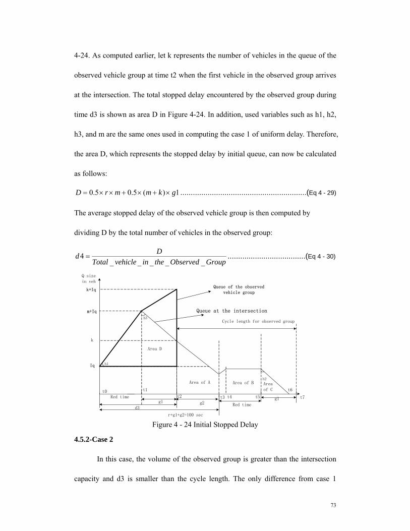
4-24. As computed earlier, let k represents the number of vehicles in the queue of the
observed vehicle group at time t2 when the first vehicle in the observed group arrives
at the intersection. The total stopped delay encountered by the observed group during
time d3 is shown as area D in Figure 4-24. In addition, used variables such as h1, h2,
h3, and m are the same ones used in computing the case 1 of uniform delay. Therefore,
the area D, which represents the stopped delay by initial queue, can now be calculated
as follows:
1)(5.05.0 gkmmrD ×+×+××= ............................................................(Eq 4 - 29)
The average stopped delay of the observed vehicle group is then computed by
dividing D by the total number of vehicles in the observed group:
GroupObservedtheinvehicleTotalDd
_____4 = .....................................(Eq 4 - 30)
Red timeg1 g2 Red time
g1
d3
m+Iq
r+g1+g2=100 sec
h2
Cycle length for observed group
Q sizein veh
t2
Area of A Area of B
t3 t4
t6
t7
Iq
t1
Queue at the intersectionh3
h1
k
t5
Areaof Ct0
k+IqQueue of the observed
vehicle group
Area D
Figure 4 - 24 Initial Stopped Delay
4.5.2-Case 2
In this case, the volume of the observed group is greater than the intersection
capacity and d3 is smaller than the cycle length. The only difference from case 1

74
above is that we need to recompute the variables h1, h2, h3, k and m based on the
detected volume instead of intersection capacity using the same algorithms as stated
before. The use of intersection capacity as the incoming volume will under-estimate
the stopped delay.
After recomputing k and m, area D, which represents the stopped delay caused
by the initial queue, is similarly calculated as follows.
1)(5.05.0 gkmmrD ×+×+××= ............................................................(Eq 4 - 31)
Consequently, the average stopped delay of the observed vehicle group is computed
as follows:
GroupObservedtheinvehicleTotalDd
_____4 = .....................................(Eq 4 - 32)
4.5.3-Case 3
In this case, d3 is greater than the Cycle Length (CL), which means that none
of the vehicles in the observed group will dissipate during this time interval as shown
in Figure 4-25. Let us assume that all vehicles in the observed group will join the
queue with a uniform distribution during the cycle length. Therefore, the total stopped
delay during the first cycle length time period when the first vehicle of the observed
group arrives at the end of initial queue can be computed as follows:
25.05.0 CLVCLCLV ××=××× ..............................................................(Eq 4 - 33)
In addition, all vehicles in the observed group will experience additional
stopped delay which is CLd −3 .
Therefore, the average stopped delay by initial queue in this case can be

75
computed as follows:
CLdCLdCLV
CLVd ×−=−+×××
= 5.0335.042
.....................................................(Eq 4 - 34)
Red time Red timeg1 g2 r g1
Cycle length
m
d3
h2
i
A B
C
h2
D
Figure 4-25 Initial Delay Case 3