Chapter 4 Clustering Algorithms and Evaluations · Clustering Algorithms and Evaluations There is a huge number of clustering algorithms and also numerous possibilities for evaluating

Chapter 4

Clustering Algorithms and Evaluations

There is a huge number of clustering algorithms and also numerous possibilities for evaluatinga clustering against a gold standard. The choice of a suitable clustering algorithm and of asuitable measure for the evaluation depends on the clustering objects and the clustering task. Theclustering objects within this thesis are verbs, and the clustering task is a semantic classificationof the verbs. Further cluster parameters are to be explored within the cluster analysis of the verbs.

This chapter provides an overview of clustering algorithmsand evaluation methods which arerelevant for the natural language clustering task of clustering verbs into semantic classes. Sec-tion 4.1 introduces clustering theory and relates the theoretical assumptions to the induction ofverb classes. Section 4.2 describes a range of possible evaluation methods and determines rele-vant measures for a verb classification. The theoretical assumptions in this chapter are the basisfor the clustering experiments in the following Chapter 5.

4.1 Clustering Theory

The section starts with an introduction into clustering theory in Section 4.1.1. Section 4.1.2 re-lates the theoretical definitions of data objects, clustering purpose and object features to verbs asthe clustering target within this thesis, and Section 4.1.3concentrates on the notion of similaritywithin the clustering of verbs. Finally, Section 4.1.4 defines the clustering algorithms as used inthe clustering experiments and refers to related clustering approaches. For more details on clus-tering theory and other clustering applications than the verb classification, the interested readeris referred to the relevant clustering literature, such as Anderberg (1973); Duda and Hart (1973);Steinhausen and Langer (1977); Jain and Dubes (1988); Kaufman and Rousseeuw (1990); Jainet al. (1999); Dudaet al. (2000).

179

180 CHAPTER 4. CLUSTERING ALGORITHMS AND EVALUATIONS

4.1.1 Introduction

Clustering is a standard procedure in multivariate data analysis. It is designed to explore an in-herent natural structure of the data objects, where objectsin the same cluster are as similar aspossible and objects in different clusters are as dissimilar as possible. The equivalence classesinduced by the clusters provide a means for generalising over the data objects and their fea-tures. Clustering methods are applied in many domains, suchas medical research, psychology,economics and pattern recognition.

Human beings often perform the task of clustering unconsciously; for example when looking at atwo-dimensional map one automatically recognises different areas according to how close to eachother the places are located, whether places are separated by rivers, lakes or a sea, etc. However,if the description of objects by their features reaches higher dimensions, intuitive judgements areless easy to obtain and justify.

The termclusteringis often confused with aclassificationor a discriminant analysis. But thethree kinds of data analyses refer to different ideas and aredistinguished as follows: Cluster-ing is (a) different from a classification, because classification assigns objects to already definedclasses, whereas for clustering no a priori knowledge aboutthe object classes and their mem-bers is provided. And a cluster analysis is (b) different from a discriminant analysis, since dis-criminant analysis aims to improve an already provided classification by strengthening the classdemarcations, whereas the cluster analysis needs to establish the class structure first.

Clustering is an exploratory data analysis. Therefore, theexplorer might have no or little infor-mation about the parameters of the resulting cluster analysis. In typical uses of clustering thegoal is to determine all of the following:� The number of clusters,� The absolute and relative positions of the clusters,� The size of the clusters,� The shape of the clusters,� The density of the clusters.

The cluster properties are explored in the process of the cluster analysis, which can be split intothe following steps.

1. Definition of objects: Which are the objects for the cluster analysis?

2. Definition of clustering purpose: What is the interest in clustering the objects?

3. Definition of features: Which are the features that describe the objects?

4. Definition of similarity measure: How can the objects be compared?

5. Definition of clustering algorithm: Which algorithm is suitable for clustering the data?

6. Definition of cluster quality: How good is the clustering result? What is the interpretation?

4.1. CLUSTERING THEORY 181

Depending on the research task, some of the steps might be naturally given by the task, othersare not known in advance. Typically, the understanding of the analysis develops iteratively withthe experiments. The following sections define a cluster analysis with respect to the task ofclustering verbs into semantic classes.

4.1.2 Data Objects, Clustering Purpose and Object Features

This work is concerned with inducing a classification of German verbs, i.e. the data objectsin the clustering experiments areGerman verbs, and the clustering purpose is to investigatethe automatic acquisition of a linguistically appropriatesemantic classificationof the verbs.The degree of appropriateness is defined with respect to the ideas of a verb classification at thesyntax-semantic interface in Chapter 2.

Once the clustering target has been selected, the objects need an attribute description as basisfor comparison. The properties are grasped by the data features, which describe the objectsin as many dimensions as necessary for the object clustering. The choice of features is of ex-treme importance, since different features might lead to different clustering results. Kaufman andRousseeuw (1990, page 14) emphasise the importance by stating that ‘a variable not containingany relevant information is worse than useless, because it will make the clustering less apparentby hiding the useful information provided by the other variables’.

Possible features to describe German verbs might include any kind of information which helpsclassify the verbs in a semantically appropriate way. Thesefeatures include the alternation be-haviour of the verbs, their morphological properties, their auxiliary selection, adverbial combi-nations, etc. Within this thesis, I concentrate on defining the verb features with respect to thealternation behaviour, because I consider thealternation behaviour a key component for verbclasses as defined in Chapter 2. So I rely on the meaning-behaviour relationship for verbs anduse empirical verb properties at thesyntax-semantic interfaceto describe the German verbs.

The verbs are described on three levels at the syntax-semantic interface, each of them refiningthe previous level by additional information. The first level encodes a purely syntactic definitionof verb subcategorisation, the second level encodes a syntactico-semantic definition of subcate-gorisation with prepositional preferences, and the third level encodes a syntactico-semantic def-inition of subcategorisation with prepositional and selectional preferences. So the refinement ofverb features starts with a purely syntactic definition and step-wise adds semantic information.The most elaborated description comes close to a definition of the verb alternation behaviour. Ihave decided on this three step proceeding of verb descriptions, because the resulting clusters andeven more the changes in clustering results which come with achange of features should pro-vide insight into the meaning-behaviour relationship at the syntax-semantic interface. The exactchoice of the features is presented and discussed in detail in the experiment setup in Chapter 5.

The representation of the verbs is realised by vectors whichdescribe the verbs by distributionsover their features. As explained in Chapter 1, the distributional representation of features for


natural language objects is widely used and has been justified by Harris (1968). The featurevalues for the distributions are provided by the German grammar, as described in Chapter 3. Thedistributions refer to (i) real valuesf representing frequencies of the features with0 � f , (ii)real valuesp representing probabilities of the features with0 � p � 1, and (iii) binary valuesb with b 2 f0; 1g. Generally speaking, a standardisation of measurement units which convertsthe original measurements (such as frequencies) to unitless variables (such as probabilities) onthe one hand may be helpful by avoiding the preference of a specific unit, but on the other handmight dampen the clustering structure by eliminating the absolute value of the feature.

4.1.3 Data Similarity Measures

With the data objects and their features specified, a means for comparing the objects is needed.The German verbs are described by features at the syntax-semantic interface, and the features arerepresented by a distributional feature vector. A range of measures calculates either the distanced or the similaritysim between two objectsx andy. The notions of ‘distance’ and ‘similarity’are related, since the smaller the distance between two objects, the more similar they are to eachother. All measures refer to the feature values in some way, but they consider different propertiesof the feature vector. There is no optimal similarity measure, since the usage depends on the task.Following, I present a range of measures which are commonly used for calculating the similarityof distributional objects. I will use all of the measures in the clustering experiments.

Minkowski Metric The Minkowski metricor Lq norm calculates the distanced between thetwo objectsx and y by comparing the values of theirn features, cf. Equation (4.1). TheMinkowski metric can be applied to frequency, probability and binary values.d(x; y) = Lq(x; y) = qvuut nXi=1 (xi � yi)q (4.1)

Two important special cases of the Minkowski metric areq = 1 andq = 2, cf. Equations (4.2)and (4.3).� Manhattan distanceor City block distanceorL1 norm:d(x; y) = L1 = nXi=1 jxi � yij (4.2)� Euclidean distanceorL2 norm:d(x; y) = L2 =vuut nXi=2 (xi � yi)2 (4.3)


Kullback-Leibler Divergence The Kullback-Leibler divergence (KL)or relative entropyisdefined in Equation (4.4). KL is a measure from information theory which determines the inef-ficiency of assuming a model distribution given the true distribution (Cover and Thomas, 1991).It is generally used forx andy representing probability mass functions, but I will also apply themeasure to probability distributions with

Pi xi > 1 andPi yi > 1.d(x; y) = D(xjjy) = nXi=1 xi � log xiyi (4.4)

The Kullback-Leibler divergence is not defined in caseyi = 0, so the probability distributionsneed to be smoothed. Two variants of KL,information radiusin Equation (4.5) andskew diver-gencein Equation (4.6), perform a default smoothing. Both variants can tolerate zero values inthe distribution, because they work with a weighted averageof the two distributions compared.Lee (2001) has recently shown that the skew divergence is an effective measure for distributionalsimilarity in NLP. Related to Lee, I set the weightw for the skew divergence to 0.9.d(x; y) = IRad(x; y) = D(xjjx+ y2 ) + D(yjjx+ y2 ) (4.5)d(x; y) = Skew(x; y) = D(xjjw � y + (1� w) � x) (4.6)� coefficient Kendall’s� coefficient(Kendall, 1993) compares all feature pairs of the two ob-jectsx andy in order to calculate their distance. Ifhxi; yii and hxj; yji are two pairs of thefeaturesi andj for the objectsx andy, the pairs are concordant ifxi > xj andyi > yj or ifxi < xj andyi < yj, and the pairs are discordant ifxi > xj andyi < yj or if xi < xj andyi > yj.If the distributions of the two objects are similar, a large number of concordancesfc is expected,otherwise a large number of discordancesfd is expected.� is defined in Equation (4.7), withpc the probability of concordances andpd the probability of discordances;� ranges from -1 to1. The� coefficient can be applied to frequency and probability values. Hatzivassiloglou andMcKeown (1993) use� to measure the similarity between adjectives.sim(x; y) = �(x; y) = fcfc + fd � fdfc + fd = pc � pd (4.7)

Cosine cos(x; y) measures the similarity of the two objectsx andy by calculating thecosine ofthe anglebetween their feature vectors. The degrees of similarity range from�1 (highest degreeof dissimilarity with vector angle =180�) over0 (angle =90�) to 1 (highest degree of similaritywith vector angle =0�). For positive feature values, the cosine lies between 0 and1. The cosinemeasure can be applied to frequency, probability and binaryvalues.sim(x; y) = cos(x; y) = Pni=1 xi � yipPni=1 x2i �pPni=1 y2i (4.8)


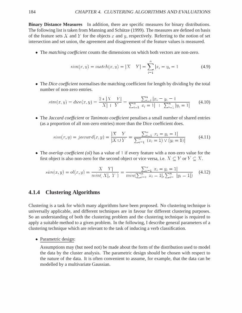
Binary Distance Measures In addition, there are specific measures for binary distributions.The following list is taken from Manning and Schütze (1999).The measures are defined on basisof the feature setsX andY for the objectsx andy, respectively. Referring to the notion of setintersection and set union, the agreement and disagreementof the feature values is measured.� Thematching coefficientcounts the dimensions on which both vectors are non-zero.sim(x; y) = match(x; y) = jX \ Y j = nXi=1 jxi = yi = 1j (4.9)� TheDice coefficientnormalises the matching coefficient for length by dividing by the total

number of non-zero entries.sim(x; y) = dice(x; y) = 2 � jX \ Y jjXj+ jY j = Pni=1 jxi = yi = 1jPni=1 jxi = 1j + Pni=1 jyi = 1j (4.10)� TheJaccard coefficientor Tanimoto coefficientpenalises a small number of shared entries(as a proportion of all non-zero entries) more than the Dice coefficient does.sim(x; y) = jaccard(x; y) = jX \ Y jjX [ Y j = Pni=1 jxi = yi = 1jPni=1 j(xi = 1) _ (yi = 1)j (4.11)� Theoverlap coefficient (ol)has a value of1 if every feature with a non-zero value for thefirst object is also non-zero for the second object or vice versa, i.e.X � Y or Y � X.sim(x; y) = ol(x; y) = jX \ Y jmin(jXj; jY j) = Pni=1 jxi = yi = 1jmin(Pni=1 jxi = 1j;Pni=1 jyi = 1j) (4.12)

4.1.4 Clustering Algorithms

Clustering is a task for which many algorithms have been proposed. No clustering technique isuniversally applicable, and different techniques are in favour for different clustering purposes.So an understanding of both the clustering problem and the clustering technique is required toapply a suitable method to a given problem. In the following,I describe general parameters of aclustering technique which are relevant to the task of inducing a verb classification.� Parametric design:

Assumptions may (but need not) be made about the form of the distribution used to modelthe data by the cluster analysis. The parametric design should be chosen with respect tothe nature of the data. It is often convenient to assume, for example, that the data can bemodelled by a multivariate Gaussian.

4.1. CLUSTERING THEORY 185� Position, size, shape and density of the clusters:

The experimenter might have an idea about the desired clustering results with respect tothe position, size, shape and density of the clusters. Different clustering algorithms havedifferent impact on these parameters, as the description ofthe algorithms will show. There-fore, varying the clustering algorithm influences the design parameters.� Number of clusters:

The number of clusters can be fixed if the desired number is known beforehand (e.g. be-cause of a reference to a gold standard), or can be varied to find the optimal cluster analysis.As Dudaet al. (2000) state, ‘In theory, the clustering problem can be solved by exhaustiveenumeration, since the sample set is finite, so there are onlya finite number of possiblepartitions; in practice, such an approach is unthinkable for all but the simplest problems,since there are at the order ofknk! ways of partitioning a set ofn elements intok subsets’.� Ambiguity:

Verbs can have multiple senses, requiring them being assigned to multiple classes. Thisis only possible by using a soft clustering algorithm, whichdefines cluster membershipprobabilities for the clustering objects. A hard clustering algorithm performs ayes/nodecision on object membership and cannot model verb ambiguity, but it is easier to useand interpret.

The choice of a clustering algorithm determines the settingof the parameters. In the followingparagraphs, I describe a range of clustering algorithms andtheir parameters. The algorithms aredivided into (A) hierarchical clustering algorithms and (B) partitioning clustering algorithms.For each type, I concentrate on the algorithms used in this thesis and refer to further possibilities.

A) Hierarchical Clustering

Hierarchical clustering methods impose a hierarchical structure on the data objects and theirstep-wise clusters, i.e. one extreme of the clustering structure is only one cluster containing allobjects, the other extreme is a number of clusters which equals the number of objects. To obtaina certain numberk of clusters, the hierarchy is cut at the relevant depth. Hierarchical clusteringis a rigid procedure, since it is not possible to re-organiseclusters established in a previous step.The original concept of a hierarchy of clusters creates hardclusters, but as e.g. Lee (1997) showsthat the concept may be transferred to soft clusters.

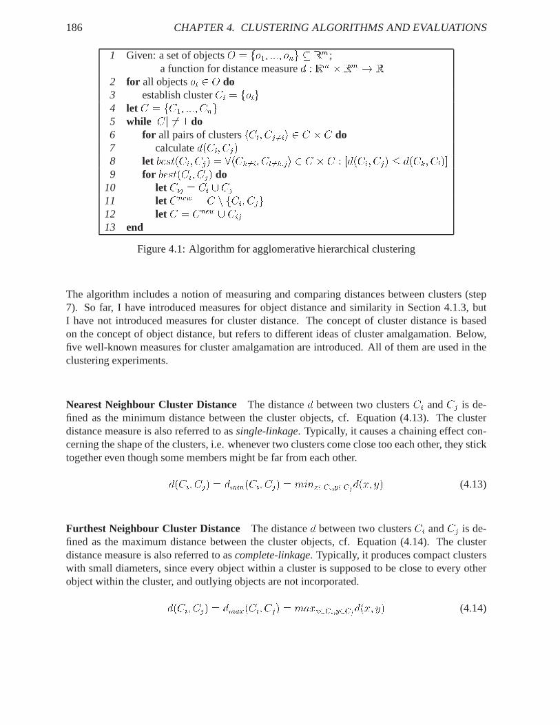
Depending on whether the clustering is performed top-down,i.e. from a single cluster to themaximum number of clusters, or bottom-up, i.e. from the maximum number of clusters to asingle cluster, we distinguish divisive and agglomerativeclustering. Divisive clustering is com-putationally more problematic than agglomerative clustering, because it needs to consider allpossible divisions into subsets. Therefore, only agglomerative clustering methods are applied inthis thesis. The algorithm is described in Figure 4.1.


1 Given: a set of objectsO = fo1; :::; ong � Rm ;a function for distance measured : Rm � Rm ! R

2 for all objectsoi 2 O do3 establish clusterCi = foig4 let C = fC1; :::; Cng5 while jCj 6= 1 do6 for all pairs of clustershCi; Cj 6=ii 2 C � C do7 calculated(Ci; Cj)8 let best(Ci; Cj) = 8hCk 6=i; Cl 6=k;ji 2 C � C : [d(Ci; Cj) � d(Ck; Cl)]9 for best(Ci; Cj) do

10 let Cij = Ci [ Cj11 let Cnew = C n fCi; Cjg12 let C = Cnew [ Cij13 end

Figure 4.1: Algorithm for agglomerative hierarchical clustering

The algorithm includes a notion of measuring and comparing distances between clusters (step7). So far, I have introduced measures for object distance and similarity in Section 4.1.3, butI have not introduced measures for cluster distance. The concept of cluster distance is basedon the concept of object distance, but refers to different ideas of cluster amalgamation. Below,five well-known measures for cluster amalgamation are introduced. All of them are used in theclustering experiments.

Nearest Neighbour Cluster Distance The distanced between two clustersCi andCj is de-fined as the minimum distance between the cluster objects, cf. Equation (4.13). The clusterdistance measure is also referred to assingle-linkage. Typically, it causes a chaining effect con-cerning the shape of the clusters, i.e. whenever two clusters come close too each other, they sticktogether even though some members might be far from each other.d(Ci; Cj) = dmin(Ci; Cj) = minx2Ci;y2Cjd(x; y) (4.13)

Furthest Neighbour Cluster Distance The distanced between two clustersCi andCj is de-fined as the maximum distance between the cluster objects, cf. Equation (4.14). The clusterdistance measure is also referred to ascomplete-linkage. Typically, it produces compact clusterswith small diameters, since every object within a cluster issupposed to be close to every otherobject within the cluster, and outlying objects are not incorporated.d(Ci; Cj) = dmax(Ci; Cj) = maxx2Ci;y2Cjd(x; y) (4.14)


Distance between Cluster Centroids The distanced between two clustersCi andCj is definedas the distance between the cluster centroidsceni andcenj, cf. Equation (4.15). The centroid ofa cluster is determined as the average of objects in the cluster, i.e. each feature of the centroidvector is calculated as the average feature value of the vectors of all objects in the cluster. Thecluster distance measure is a natural compromise between the nearest and the furthest neighbourcluster distance approaches. Different to the above approaches, it does not impose a structure onthe clustering effect. d(Ci; Cj) = dmean(Ci; Cj) = d(ceni; cenj) (4.15)

Average Distance between Clusters The distanced between two clustersci andcj is definedas the average distance between the cluster objects, cf. Equation (4.16). Likedmean, the clusterdistance measure is a natural compromise between the nearest and the furthest neighbour clusterdistance approaches. It does not impose a structure on the clustering effect either.d(Ci; Cj) = davg(Ci; Cj) = 1jCij � jCjj � Xx2Ci Xy2Cj d(x; y) (4.16)

Ward’s Method The distanced between two clustersCi andCj is defined as the loss of infor-mation (or: the increase in error) in merging two clusters (Ward, 1963), cf. Equation (4.17). Theerror of a clusterC is measured as the sum of distances between the objects in thecluster and thecluster centroidcenC . When merging two clusters, the error of the merged cluster is larger thanthe sum or errors of the two individual clusters, and therefore represents a loss of information.But the merging is performed on those clusters which are mosthomogeneous, to unify clusterssuch that the variation inside the merged clusters increases as little as possible. Ward’s methodtends to create compact clusters of small size. It is a least squares method, so implicitly assumesa Gaussian model.d(Ci; Cj) = dward(Ci; Cj) = Xx2(Ci[Cj) d(x; cenij) � [Xx2Ci d(x; ceni) + Xx2cenj d(x; cenj)]

(4.17)

B) Partitioning Clustering

Partitioning clustering methods partition the data objectset into clusters where every pair of ob-ject clusters is either distinct (hard clustering) or has some members in common (soft clustering).Partitioning clustering begins with a starting cluster partition which is iteratively improved untila locally optimal partition is reached. The starting clusters can be either random or the clusteroutput from some clustering pre-process (e.g. hierarchical clustering). In the resulting clusters,the objects in the groups together add up to the full object set.


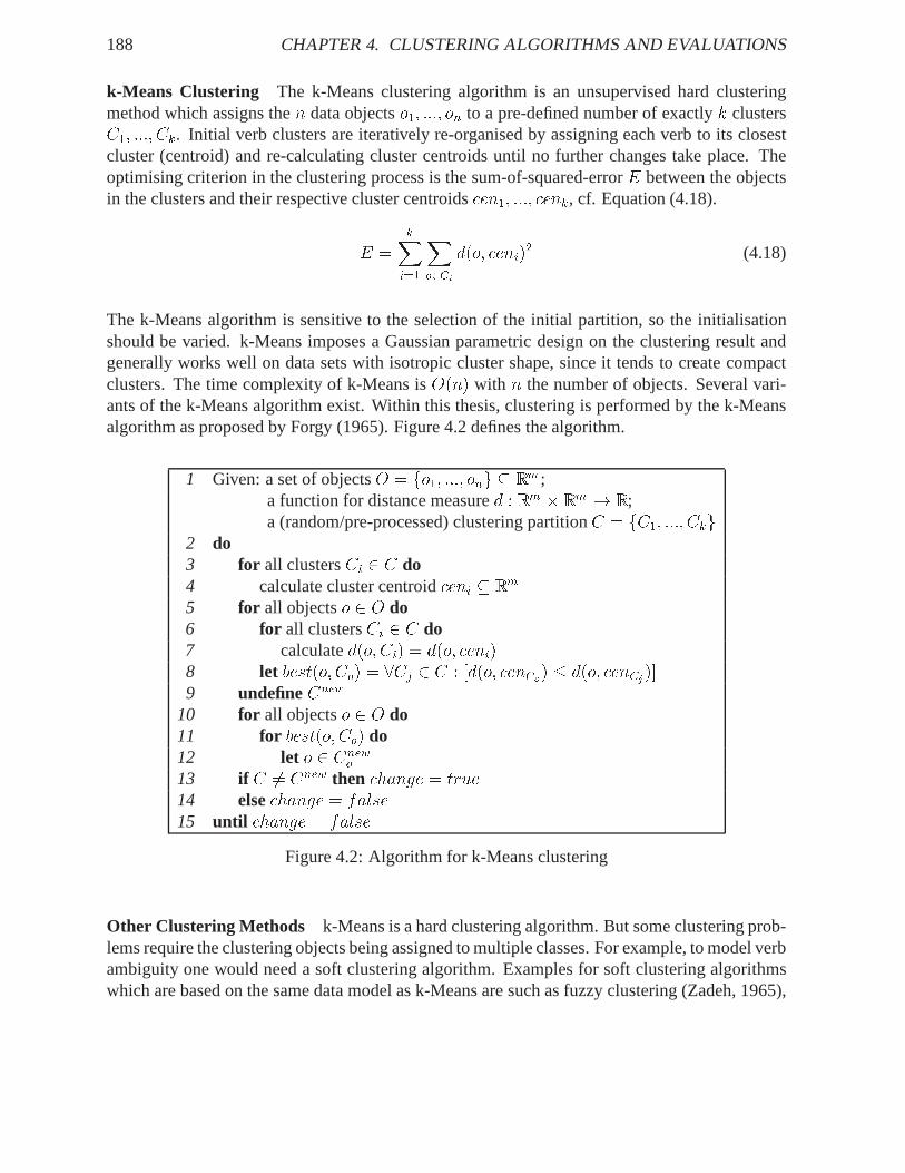
k-Means Clustering The k-Means clustering algorithm is an unsupervised hard clusteringmethod which assigns then data objectso1; :::; on to a pre-defined number of exactlyk clustersC1; :::; Ck. Initial verb clusters are iteratively re-organised by assigning each verb to its closestcluster (centroid) and re-calculating cluster centroids until no further changes take place. Theoptimising criterion in the clustering process is the sum-of-squared-errorE between the objectsin the clusters and their respective cluster centroidscen1; :::; cenk, cf. Equation (4.18).E = kXi=1 Xo2Ci d(o; ceni)2 (4.18)

The k-Means algorithm is sensitive to the selection of the initial partition, so the initialisationshould be varied. k-Means imposes a Gaussian parametric design on the clustering result andgenerally works well on data sets with isotropic cluster shape, since it tends to create compactclusters. The time complexity of k-Means isO(n) with n the number of objects. Several vari-ants of the k-Means algorithm exist. Within this thesis, clustering is performed by the k-Meansalgorithm as proposed by Forgy (1965). Figure 4.2 defines thealgorithm.

1 Given: a set of objectsO = fo1; :::; ong � Rm ;a function for distance measured : Rm � Rm ! R;a (random/pre-processed) clustering partitionC = fC1; :::; Ckg

2 do3 for all clustersCi 2 C do4 calculate cluster centroidceni � Rm5 for all objectso 2 O do6 for all clustersCi 2 C do7 calculated(o; Ci) = d(o; ceni)8 let best(o; Co) = 8Cj 2 C : [d(o; cenCo) � d(o; cenCj )]9 undefineCnew

10 for all objectso 2 O do11 for best(o; Co) do12 let o 2 Cnewo13 if C 6= Cnew then change = true14 elsechange = false15 until change = false

Figure 4.2: Algorithm for k-Means clustering

Other Clustering Methods k-Means is a hard clustering algorithm. But some clusteringprob-lems require the clustering objects being assigned to multiple classes. For example, to model verbambiguity one would need a soft clustering algorithm. Examples for soft clustering algorithmswhich are based on the same data model as k-Means are such as fuzzy clustering (Zadeh, 1965),


cf. also Höppneret al. (1997) and Dudaet al. (2000), and theExpectation-Maximisation (EM)Algorithm (Baum, 1972) which can also be implemented as a soft version of k-Means with anunderlying Gaussian model.

The above methods represent a standard choice for clustering in pattern recognition, cf. Dudaet al.(2000). Clustering techniques with different background are e.g. theNearest Neighbour Al-gorithm(Jarvis and Patrick, 1973),Graph-Based Clustering(Zahn, 1971), andArtificial NeuralNetworks(Hertzet al., 1991). Recently, elaborated techniques from especially image processinghave been transfered to linguistic clustering, such asSpectral Clustering(Brew and Schulte imWalde, 2002).

C) Decision on Clustering Algorithm

Within the scope of this thesis, I apply the hard clustering technique k-Means to the German verbdata. I decided to use the k-Means algorithm for the clustering, because it is a standard clusteringtechnique with well-known properties. In addition, see thefollowing arguments.� The parametric design of Gaussian structures realises the idea that objects should belong

to a cluster if they are very similar to the centroid as the average description of the cluster,and that an increasing distance refers to a decrease in cluster membership. In addition, theisotropic shape of clusters reflects the intuition of a compact verb classification.� A variation of the clustering initialisation performs a variation of the clustering parame-ters such as position, size, shape and density of the clusters. Even though I assume thatan appropriate parametric design for the verb classification is given by isotropic clusterformation, a variation of initial clusters investigates the relationship between clusteringdata and cluster formation. I will therefore apply random initialisations and hierarchicalclusters as input to k-Means.� Selim and Ismail (1984) prove for distance metrices (a subset of the similarity measuresin Section 4.1.3) that k-Means finds locally optimal solutions by minimising the sum-of-squared-error between the objects in the clusters and theirrespective cluster centroids.� Starting clustering experiments with a hard clustering algorithm is an easier task than ap-plying a soft clustering algorithm, especially with respect to a linguistic investigation of theexperiment settings and results. Ambiguities are a difficult problem in linguistics, and aresubject to future work. I will investigate the impact of the hard clustering on polysemousverbs, but not try to model the polysemy within this work.� As to the more general question whether to use a supervised classification or an unsuper-vised clustering method, this work concentrates on minimising the manual interventionin the automatic class acquisition. A classification would require costly manual labelling(especially with respect to a large-scale classification) and not agree with the exploratorygoal of finding as many independent linguistic insights as possible at the syntax-semanticinterface of verb classifications.


4.2 Clustering Evaluation

A clustering evaluation demands an independent and reliable measure for the assessment andcomparison of clustering experiments and results. In theory, the clustering researcher has ac-quired an intuition for the clustering evaluation, but in practise the mass of data on the one handand the subtle details of data representation and clustering algorithms on the other hand makean intuitive judgement impossible. An intuitive, introspective evaluation can therefore only beplausible for small sets of objects, but large-scale experiments require an objective method.

There is no absolute scheme with which to measure clusterings, but a variety of evaluation mea-sures from diverse areas such as theoretical statistics, machine vision and web-page clustering areapplicable. In this section, I provide the definition of various clustering evaluation measures andevaluate them with respect to their linguistic application. Section 4.2.1 describes the demands Iexpect to fulfill with an evaluation measure on verb clusterings. In Section 4.2.2 I present a rangeof possible evaluation methods, and Section 4.2.3 comparesthe measures against each other andaccording to the evaluation demands.

4.2.1 Demands on Clustering Evaluation

An objective method for evaluating clusterings should be independent of the evaluator and reli-able concerning its judgement about the quality of the clusterings. How can we transfer theseabstract descriptions to more concrete demands? Following, I define demands on the task of clus-tering verbs into semantic classes, with an increasing proportion of linguistic task specificity. I.e.I first define general demands on an evaluation, then general demands on a clustering evaluation,and finally demands on the verb-specific clustering evaluation.

The demands on the clustering evaluation are easier described with reference to the formal nota-tion of clustering result and gold standard classification,so the notation is provided in advance:

Definition 4.1 Given an object setO = fo1; :::; ong with n objects, the clustering result and themanual classification as the gold standard represent two partitions ofO with C = fC1; :::; CkgandM = fM1;M2; :::;Mlg, respectively.Ci 2 C denotes the set of objects in theith cluster ofpartitionC, andMj 2M denotes the set of objects in thejth cluster of partitionM .

General Evaluation Demands Firstly, I define a demand on evaluation in general: The evalu-ation of an experiment should be proceeded against a gold standard, as independent and reliableas possible. My gold standard is the manual classification ofverbs, as described in Chapter 2.The classification has been created by the author. To compensate for the sub-optimal setup by asingle person, the classification was developed in close relation to the existing classifications forGerman by Schumacher (1986) and English by Levin (1993). In addition, the complete classifi-cation was finished before any experiments on the verbs were performed.

4.2. CLUSTERING EVALUATION 191

General Clustering Demands The second range of demands refers to general properties of acluster analysis, independent of the clustering area.� Since the purpose of the evaluation is to assess and compare different clustering exper-

iments and results, the measure should be applicable to all similarity measures used inclustering, but possibly independent of the respective similarity measure.� The evaluation result should define a (numerical) measure indicating the value of the clus-tering. The resulting value should either be easy to interpret or otherwise be illustratedwith respect to its range and effects, in order to facilitatethe evaluation interpretation.� The evaluation method should be defined without a bias towards a specific number andsize of clusters.� The evaluation measure should distinguish the quality of (i) the whole clustering partitionC, and (ii) the specific clustersCi 2 C.

Linguistic Clustering Demands The fact that this thesis is concerned with the clustering oflinguistic data sharpens the requirements on an appropriate clustering evaluation, because thedemands on verb classes are specific to the linguistic background and linguistic intuition and notnecessarily desired for different clustering areas. The following list therefore refers to a thirdrange of demands, defined as linguistic desiderata for the clustering of verbs.

(a) The clustering result should not be a single cluster representing the clustering partition, i.e.jCj = 1. A single cluster does not represent an appropriate model for verb classes.

(b) The clustering result should not be a clustering partition with only singletons, i.e.8Ci 2 C :jCij = 1. A set of singletons does not represent an appropriate modelfor verb classes either.

(c) Let Ci be a correct (according to the gold standard) cluster withjCij = x. Compare thiscluster with the correct clusterCj with jCjj = y > x. The evaluated quality ofCj shouldbe better compared toCi, since the latter cluster was able to create a larger correctcluster,which is a more difficult task.

Example:1 Ci = ahnen vermuten wissenCj = ahnen denken glauben vermuten wissen

(d) LetCi be a correct cluster andCj be a cluster which is identical toCi, but contains additionalobjects which do not belong to the same class. The evaluated quality of Ci should be bettercompared toCj, since the former cluster contains fewer errors.

Example: Ci = ahnen vermuten wissenCj = ahnen vermuten wissenlaufen lachen

1In all examples, verbs belonging to the same gold standard class are underlined in the cluster.


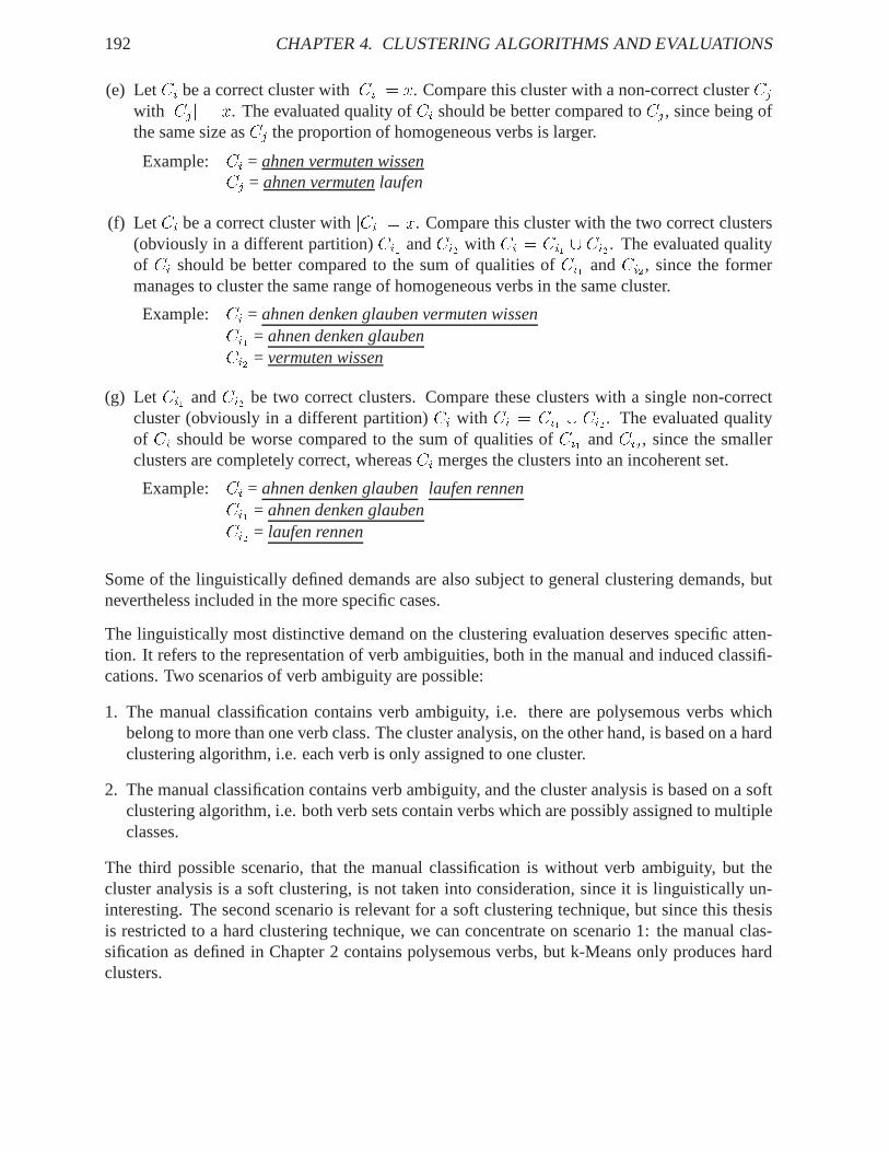
(e) LetCi be a correct cluster withjCij = x. Compare this cluster with a non-correct clusterCjwith jCjj = x. The evaluated quality ofCi should be better compared toCj, since being ofthe same size asCj the proportion of homogeneous verbs is larger.

Example: Ci = ahnen vermuten wissenCj = ahnen vermutenlaufen

(f) Let Ci be a correct cluster withjCij = x. Compare this cluster with the two correct clusters(obviously in a different partition)Ci1 andCi2 with Ci = Ci1 [ Ci2 . The evaluated qualityof Ci should be better compared to the sum of qualities ofCi1 andCi2 , since the formermanages to cluster the same range of homogeneous verbs in thesame cluster.

Example: Ci = ahnen denken glauben vermuten wissenCi1 = ahnen denken glaubenCi2 = vermuten wissen

(g) Let Ci1 andCi2 be two correct clusters. Compare these clusters with a single non-correctcluster (obviously in a different partition)Ci with Ci = Ci1 [ Ci2 . The evaluated qualityof Ci should be worse compared to the sum of qualities ofCi1 andCi2 , since the smallerclusters are completely correct, whereasCi merges the clusters into an incoherent set.

Example: Ci = ahnen denken glaubenlaufen rennenCi1 = ahnen denken glaubenCi2 = laufen rennen

Some of the linguistically defined demands are also subject to general clustering demands, butnevertheless included in the more specific cases.

The linguistically most distinctive demand on the clustering evaluation deserves specific atten-tion. It refers to the representation of verb ambiguities, both in the manual and induced classifi-cations. Two scenarios of verb ambiguity are possible:

1. The manual classification contains verb ambiguity, i.e. there are polysemous verbs whichbelong to more than one verb class. The cluster analysis, on the other hand, is based on a hardclustering algorithm, i.e. each verb is only assigned to onecluster.

2. The manual classification contains verb ambiguity, and the cluster analysis is based on a softclustering algorithm, i.e. both verb sets contain verbs which are possibly assigned to multipleclasses.

The third possible scenario, that the manual classificationis without verb ambiguity, but thecluster analysis is a soft clustering, is not taken into consideration, since it is linguistically un-interesting. The second scenario is relevant for a soft clustering technique, but since this thesisis restricted to a hard clustering technique, we can concentrate on scenario 1: the manual clas-sification as defined in Chapter 2 contains polysemous verbs,but k-Means only produces hardclusters.


4.2.2 Description of Evaluation Measures

In the following, I describe a range of possible evaluation measures, with different theoreticalbackgrounds and demands. The overview does, of course, not represent an exhaustive list ofclustering evaluations, but tries to give an impression of the variety of possible methods whichare concerned with clustering and clustering evaluation. Not all of the described measures areapplicable to our clustering task, so a comparison and choice of the candidate methods will beprovided in Section 4.2.3.

Contingency Tables Contingency tables are a typical means for describing and defining theassociation between two partitions. As they will be of use ina number of evaluation examplesbelow, their notation is given beforehand.

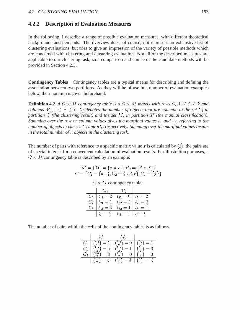
Definition 4.2 A C �M contingency table is aC �M matrix with rowsCi; 1 � i � k andcolumnsMj; 1 � j � l. tij denotes the number of objects that are common to the setCi inpartition C (the clustering result) and the setMj in partition M (the manual classification).Summing over the row or column values gives the marginal valuesti: and t:j, referring to thenumber of objects in classesCi andMj, respectively. Summing over the marginal values resultsin the total number ofn objects in the clustering task.

The number of pairs with reference to a specific matrix valuex is calculated by�x2�; the pairs are

of special interest for a convenient calculation of evaluation results. For illustration purposes, aC �M contingency table is described by an example:M = fM1 = fa; b; cg;M2 = fd; e; fggC = fC1 = fa; bg; C2 = fc; d; eg; C3 = ffggC �M contingency table:M1 M2C1 t11 = 2 t12 = 0 t1: = 2C2 t21 = 1 t22 = 2 t2: = 3C3 t31 = 0 t32 = 1 t3: = 1t:1 = 3 t:2 = 3 n = 6The number of pairs within the cells of the contingency tables is as follows.M1 M2C1 �t112 � = 1 �t122 � = 0 �t1:2 � = 1C2 �t212 � = 0 �t222 � = 1 �t2:2 � = 3C3 �t312 � = 0 �t322 � = 0 �t3:2 � = 0�t:12 � = 3 �t:22 � = 3 �n2� = 15


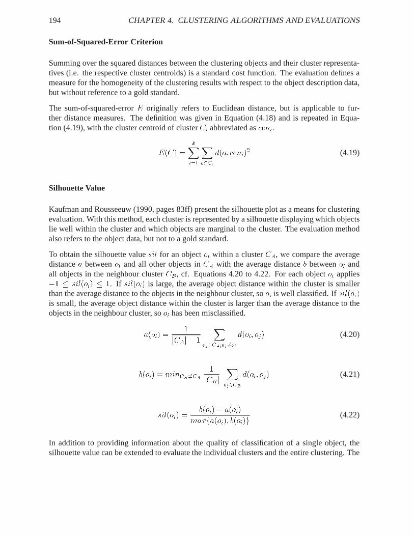
Sum-of-Squared-Error Criterion

Summing over the squared distances between the clustering objects and their cluster representa-tives (i.e. the respective cluster centroids) is a standardcost function. The evaluation defines ameasure for the homogeneity of the clustering results with respect to the object description data,but without reference to a gold standard.

The sum-of-squared-errorE originally refers to Euclidean distance, but is applicableto fur-ther distance measures. The definition was given in Equation(4.18) and is repeated in Equa-tion (4.19), with the cluster centroid of clusterCi abbreviated asceni.E(C) = kXi=1 Xo2Ci d(o; ceni)2 (4.19)

Silhouette Value

Kaufman and Rousseeuw (1990, pages 83ff) present the silhouette plot as a means for clusteringevaluation. With this method, each cluster is represented by a silhouette displaying which objectslie well within the cluster and which objects are marginal tothe cluster. The evaluation methodalso refers to the object data, but not to a gold standard.

To obtain the silhouette valuesil for an objectoi within a clusterCA, we compare the averagedistancea betweenoi and all other objects inCA with the average distanceb betweenoi andall objects in the neighbour clusterCB, cf. Equations 4.20 to 4.22. For each objectoi applies�1 � sil(oi) � 1. If sil(oi) is large, the average object distance within the cluster is smallerthan the average distance to the objects in the neighbour cluster, sooi is well classified. Ifsil(oi)is small, the average object distance within the cluster is larger than the average distance to theobjects in the neighbour cluster, sooi has been misclassified.a(oi) = 1jCAj � 1 Xoj2CA;oj 6=oi d(oi; oj) (4.20)b(oi) = minCB 6=CA 1jCBj Xoj2CB d(oi; oj) (4.21)sil(oi) = b(oi)� a(oi)maxfa(oi); b(oi)g (4.22)

In addition to providing information about the quality of classification of a single object, thesilhouette value can be extended to evaluate the individualclusters and the entire clustering. The


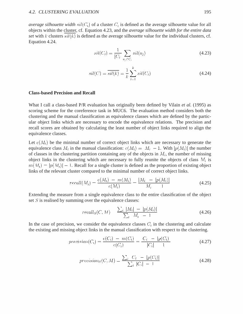
average silhouette widthsil(Ci) of a clusterCi is defined as the average silhouette value for allobjects within the cluster, cf. Equation 4.23, and theaverage silhouette width for the entire datasetwith k clusterssil(k) is defined as the average silhouette value for the individualclusters, cf.Equation 4.24. sil(Ci) = 1jCij Xoj2Ci sil(oj) (4.23)sil(C) = sil(k) = 1k kXi=1 sil(Ci) (4.24)

Class-based Precision and Recall

What I call a class-based P/R evaluation has originally beendefined by Vilainet al. (1995) asscoring scheme for the coreference task in MUC6. The evaluation method considers both theclustering and the manual classification as equivalence classes which are defined by the partic-ular object links which are necessary to encode the equivalence relations. The precision andrecall scores are obtained by calculating the least number of object links required to align theequivalence classes.

Let c(Mi) be the minimal number of correct object links which are necessary to generate theequivalence classMi in the manual classification:c(Mi) = jMij � 1. With jp(Mi)j the numberof classes in the clustering partition containing any of theobjects inMi, the number of missingobject links in the clustering which are necessary to fully reunite the objects of classMi ism(Mi) = jp(Mi)j � 1. Recall for a single cluster is defined as the proportion of existing objectlinks of the relevant cluster compared to the minimal numberof correct object links.recall(Mi) = c(Mi) � m(Mi)c(Mi) = jMij � jp(Mi)jjMij � 1 (4.25)

Extending the measure from a single equivalence class to theentire classification of the objectsetS is realised by summing over the equivalence classes:recallS(C;M) = Pi jMij � jp(Mi)jPi jMij � 1 (4.26)

In the case of precision, we consider the equivalence classesCi in the clustering and calculatethe existing and missing object links in the manual classification with respect to the clustering.precision(Ci) = c(Ci) � m(Ci)c(Ci) = jCij � jp(Ci)jjCij � 1 (4.27)precisionS(C;M) = Pi jCij � jp(Ci)jPi jCij � 1 (4.28)


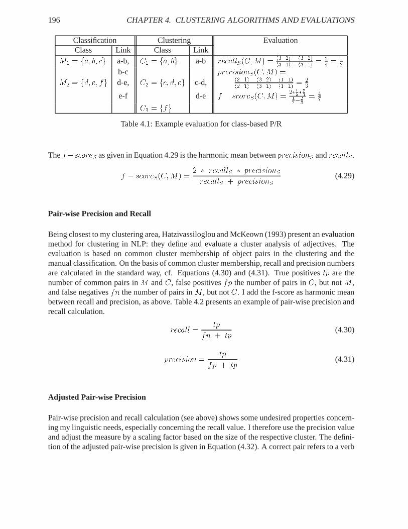
Classification Clustering EvaluationClass Link Class LinkM1 = fa; b; cg a-b, C1 = fa; bg a-b recallS(C;M) = (3�2) + (3�2)(3�1) + (3�1) = 24 = 12

b-c precisionS(C;M) =M2 = fd; e; fg d-e, C2 = fc; d; eg c-d, (2�1) + (3�2) + (1�1)(2�1) + (3�1) + (1�1) = 23e-f d-e f � scoreS(C;M) = 2� 12� 2312+ 23 = 47C3 = ffgTable 4.1: Example evaluation for class-based P/R

Thef�scoreS as given in Equation 4.29 is the harmonic mean betweenprecisionS andrecallS.f � scoreS(C;M) = 2 � recallS � precisionSrecallS + precisionS (4.29)

Pair-wise Precision and Recall

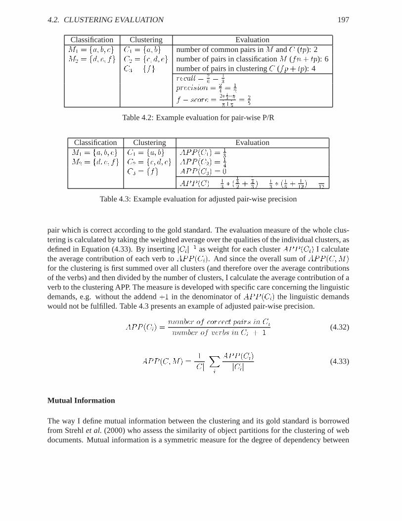
Being closest to my clustering area, Hatzivassiloglou and McKeown (1993) present an evaluationmethod for clustering in NLP: they define and evaluate a cluster analysis of adjectives. Theevaluation is based on common cluster membership of object pairs in the clustering and themanual classification. On the basis of common cluster membership, recall and precision numbersare calculated in the standard way, cf. Equations (4.30) and(4.31). True positivestp are thenumber of common pairs inM andC, false positivesfp the number of pairs inC, but notM ,and false negativesfn the number of pairs inM , but notC. I add the f-score as harmonic meanbetween recall and precision, as above. Table 4.2 presents an example of pair-wise precision andrecall calculation. recall = tpfn + tp (4.30)precision = tpfp + tp (4.31)

Adjusted Pair-wise Precision

Pair-wise precision and recall calculation (see above) shows some undesired properties concern-ing my linguistic needs, especially concerning the recall value. I therefore use the precision valueand adjust the measure by a scaling factor based on the size ofthe respective cluster. The defini-tion of the adjusted pair-wise precision is given in Equation (4.32). A correct pair refers to a verb


Classification Clustering EvaluationM1 = fa; b; cg C1 = fa; bg number of common pairs inM andC (tp): 2M2 = fd; e; fg C2 = fc; d; eg number of pairs in classificationM (fn+ tp): 6C3 = ffg number of pairs in clusteringC (fp+ tp): 4recall = 26 = 13precision = 24 = 12f � score = 2� 13� 1213+ 12 = 25Table 4.2: Example evaluation for pair-wise P/R

Classification Clustering EvaluationM1 = fa; b; cg C1 = fa; bg APP (C1) = 13M2 = fd; e; fg C2 = fc; d; eg APP (C2) = 14C3 = ffg APP (C3) = 0APP (C) = 13 � ( 132 + 143 ) = 13 � (16 + 112) = 112Table 4.3: Example evaluation for adjusted pair-wise precision

pair which is correct according to the gold standard. The evaluation measure of the whole clus-tering is calculated by taking the weighted average over thequalities of the individual clusters, asdefined in Equation (4.33). By insertingjCij�1 as weight for each clusterAPP (Ci) I calculatethe average contribution of each verb toAPP (Ci). And since the overall sum ofAPP (C;M)for the clustering is first summed over all clusters (and therefore over the average contributionsof the verbs) and then divided by the number of clusters, I calculate the average contribution of averb to the clustering APP. The measure is developed with specific care concerning the linguisticdemands, e.g. without the addend+1 in the denominator ofAPP (Ci) the linguistic demandswould not be fulfilled. Table 4.3 presents an example of adjusted pair-wise precision.APP (Ci) = number of correct pairs in Cinumber of verbs in Ci + 1 (4.32)APP (C;M) = 1jCj Xi APP (Ci)jCij (4.33)

Mutual Information

The way I define mutual information between the clustering and its gold standard is borrowedfrom Strehlet al. (2000) who assess the similarity of object partitions for the clustering of webdocuments. Mutual information is a symmetric measure for the degree of dependency between


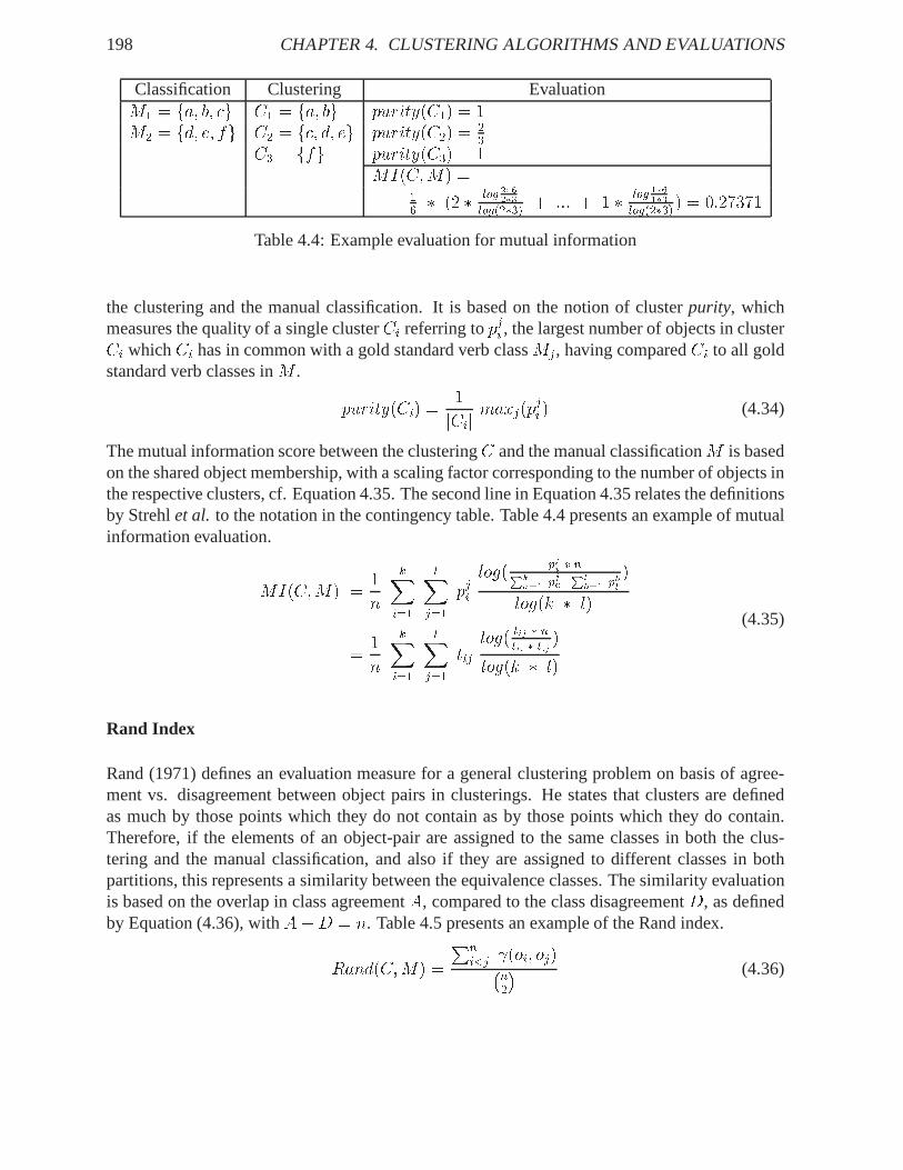
Classification Clustering EvaluationM1 = fa; b; cg C1 = fa; bg purity(C1) = 1M2 = fd; e; fg C2 = fc; d; eg purity(C2) = 23C3 = ffg purity(C3) = 1MI(C;M) =16 � (2 � log 2�62�3log(2�3) + ::: + 1 � log 1�61�3log(2�3) ) = 0:27371Table 4.4: Example evaluation for mutual information

the clustering and the manual classification. It is based on the notion of clusterpurity, whichmeasures the quality of a single clusterCi referring topji , the largest number of objects in clusterCi whichCi has in common with a gold standard verb classMj, having comparedCi to all goldstandard verb classes inM . purity(Ci) = 1jCij maxj(pji ) (4.34)

The mutual information score between the clusteringC and the manual classificationM is basedon the shared object membership, with a scaling factor corresponding to the number of objects inthe respective clusters, cf. Equation 4.35. The second linein Equation 4.35 relates the definitionsby Strehlet al. to the notation in the contingency table. Table 4.4 presentsan example of mutualinformation evaluation.MI(C;M) = 1n kXi=1 lXj=1 pji log( pji � nPka=1 pja Plb=1 pbl )log(k � l)= 1n kXi=1 lXj=1 tij log( tij � nti: � t:j )log(k � l) (4.35)

Rand Index

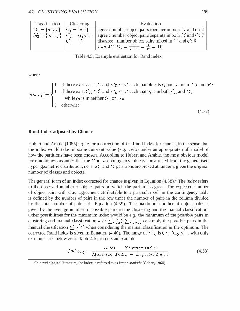
Rand (1971) defines an evaluation measure for a general clustering problem on basis of agree-ment vs. disagreement between object pairs in clusterings.He states that clusters are definedas much by those points which they do not contain as by those points which they do contain.Therefore, if the elements of an object-pair are assigned tothe same classes in both the clus-tering and the manual classification, and also if they are assigned to different classes in bothpartitions, this represents a similarity between the equivalence classes. The similarity evaluationis based on the overlap in class agreementA, compared to the class disagreementD, as definedby Equation (4.36), withA+D = n. Table 4.5 presents an example of the Rand index.Rand(C;M) = Pni<j (oi; oj)�n2� (4.36)


Classification Clustering EvaluationM1 = fa; b; cg C1 = fa; bg agree : number object pairs together in bothM andC: 2M2 = fd; e; fg C2 = fc; d; eg agree : number object pairs separate in bothM andC: 7C3 = ffg disagree : number object pairs mixed inM andC: 6Rand(C;M) = 2+72+7+6 = 915 = 0:6Table 4.5: Example evaluation for Rand index

where (oi; oj) = 8>>><>>>:1 if there existCA 2 C andMB 2M such that objectsoi andoj are inCA andMB;1 if there existCA 2 C andMB 2M such thatoi is in bothCA andMBwhile oj is in neitherCA orMB;0 otherwise:

(4.37)

Rand Index adjusted by Chance

Hubert and Arabie (1985) argue for a correction of the Rand index for chance, in the sense thatthe index would take on some constant value (e.g. zero) underan appropriate null model ofhow the partitions have been chosen. According to Hubert andArabie, the most obvious modelfor randomness assumes that theC �M contingency table is constructed from the generalisedhyper-geometric distribution, i.e. theC andM partitions are picked at random, given the originalnumber of classes and objects.

The general form of an index corrected for chance is given in Equation (4.38).2 The indexrefersto the observed number of object pairs on which the partitions agree. The expected numberof object pairs with class agreement attributable to a particular cell in the contingency tableis defined by the number of pairs in the row times the number of pairs in the column dividedby the total number of pairs, cf. Equation (4.39). The maximum number of object pairs isgiven by the average number of possible pairs in the clustering and the manual classification.Other possibilities for the maximum index would be e.g. the minimum of the possible pairs inclustering and manual classificationmin(Pi �ti:2 �;Pj �t:j2 �) or simply the possible pairs in themanual classification

Pj �t:j2 � when considering the manual classification as the optimum. Thecorrected Rand index is given in Equation (4.40). The range of Radj is 0 � Radj � 1, with onlyextreme cases below zero. Table 4.6 presents an example.Indexadj = Index � Expected IndexMaximum Index � Expected Index (4.38)

2In psychological literature, the index is referred to askappa statistic(Cohen, 1960).


Classification Clustering EvaluationM1 = fa; b; cg C1 = fa; bg Randadj = 2 � 4�61512 (4+6) � 4�615 = 2 � 855 � 85 = 0:11765M2 = fd; e; fg C2 = fc; d; egC3 = ffgTable 4.6: Example evaluation for adjusted Rand indexExp�tij2 � = �ti:2 � �t:j2 ��n2� (4.39)Randadj(C;M) = Pi;j �tij2 � � Pi (ti:2 ) Pj (t:j2 )(n2)12 (Pi �ti:2 � + Pj �t:j2 �) � Pi (ti:2 ) Pj (t:j2 )(n2) (4.40)

Matching Index

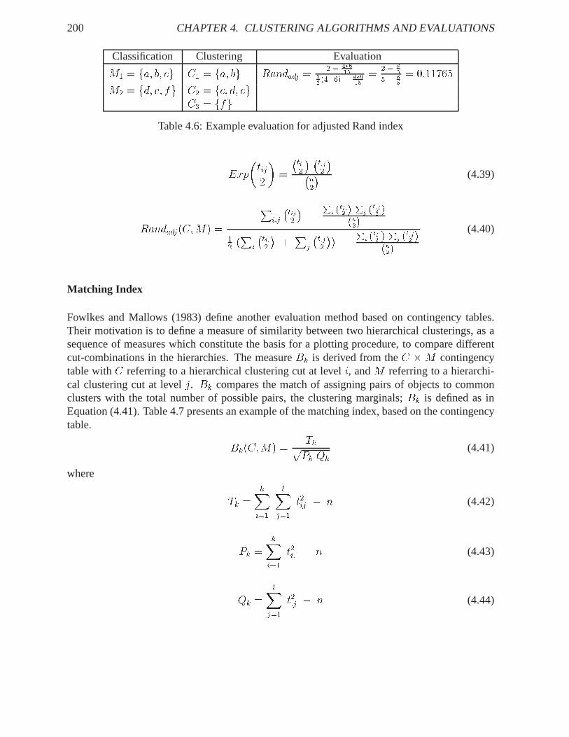
Fowlkes and Mallows (1983) define another evaluation methodbased on contingency tables.Their motivation is to define a measure of similarity betweentwo hierarchical clusterings, as asequence of measures which constitute the basis for a plotting procedure, to compare differentcut-combinations in the hierarchies. The measureBk is derived from theC �M contingencytable withC referring to a hierarchical clustering cut at leveli, andM referring to a hierarchi-cal clustering cut at levelj. Bk compares the match of assigning pairs of objects to commonclusters with the total number of possible pairs, the clustering marginals;Bk is defined as inEquation (4.41). Table 4.7 presents an example of the matching index, based on the contingencytable. Bk(C;M) = TkpPk Qk (4.41)

where Tk = kXi=1 lXj=1 t2ij � n (4.42)Pk = kXi=1 t2i: � n (4.43)Qk = lXj=1 t2:j � n (4.44)


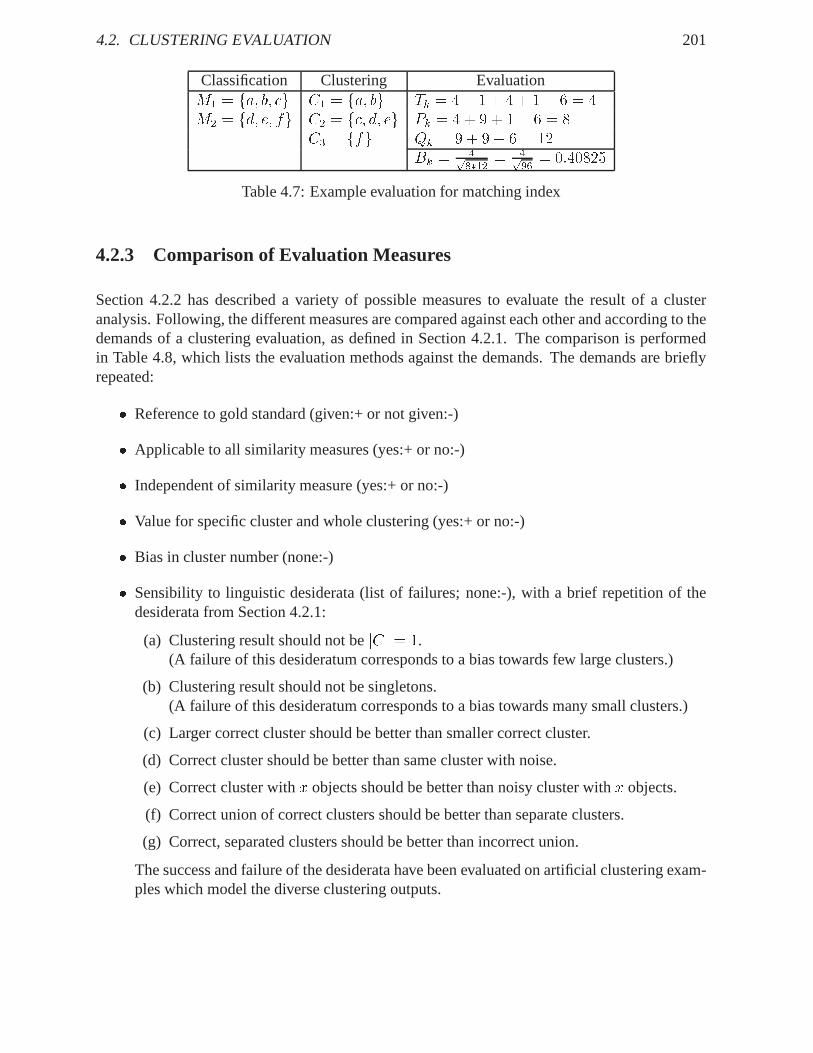
Classification Clustering EvaluationM1 = fa; b; cg C1 = fa; bg Tk = 4 + 1 + 4 + 1� 6 = 4M2 = fd; e; fg C2 = fc; d; eg Pk = 4 + 9 + 1� 6 = 8C3 = ffg Qk = 9 + 9� 6 = 12Bk = 4p8�12 = 4p96 = 0:40825Table 4.7: Example evaluation for matching index

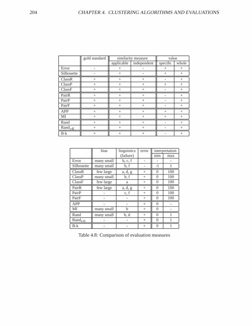
4.2.3 Comparison of Evaluation Measures

Section 4.2.2 has described a variety of possible measures to evaluate the result of a clusteranalysis. Following, the different measures are compared against each other and according to thedemands of a clustering evaluation, as defined in Section 4.2.1. The comparison is performedin Table 4.8, which lists the evaluation methods against thedemands. The demands are brieflyrepeated:� Reference to gold standard (given:+ or not given:-)� Applicable to all similarity measures (yes:+ or no:-)� Independent of similarity measure (yes:+ or no:-)� Value for specific cluster and whole clustering (yes:+ or no:-)� Bias in cluster number (none:-)� Sensibility to linguistic desiderata (list of failures; none:-), with a brief repetition of the

desiderata from Section 4.2.1:

(a) Clustering result should not bejCj = 1.(A failure of this desideratum corresponds to a bias towardsfew large clusters.)

(b) Clustering result should not be singletons.(A failure of this desideratum corresponds to a bias towardsmany small clusters.)

(c) Larger correct cluster should be better than smaller correct cluster.

(d) Correct cluster should be better than same cluster with noise.

(e) Correct cluster withx objects should be better than noisy cluster withx objects.

(f) Correct union of correct clusters should be better than separate clusters.

(g) Correct, separated clusters should be better than incorrect union.

The success and failure of the desiderata have been evaluated on artificial clustering exam-ples which model the diverse clustering outputs.

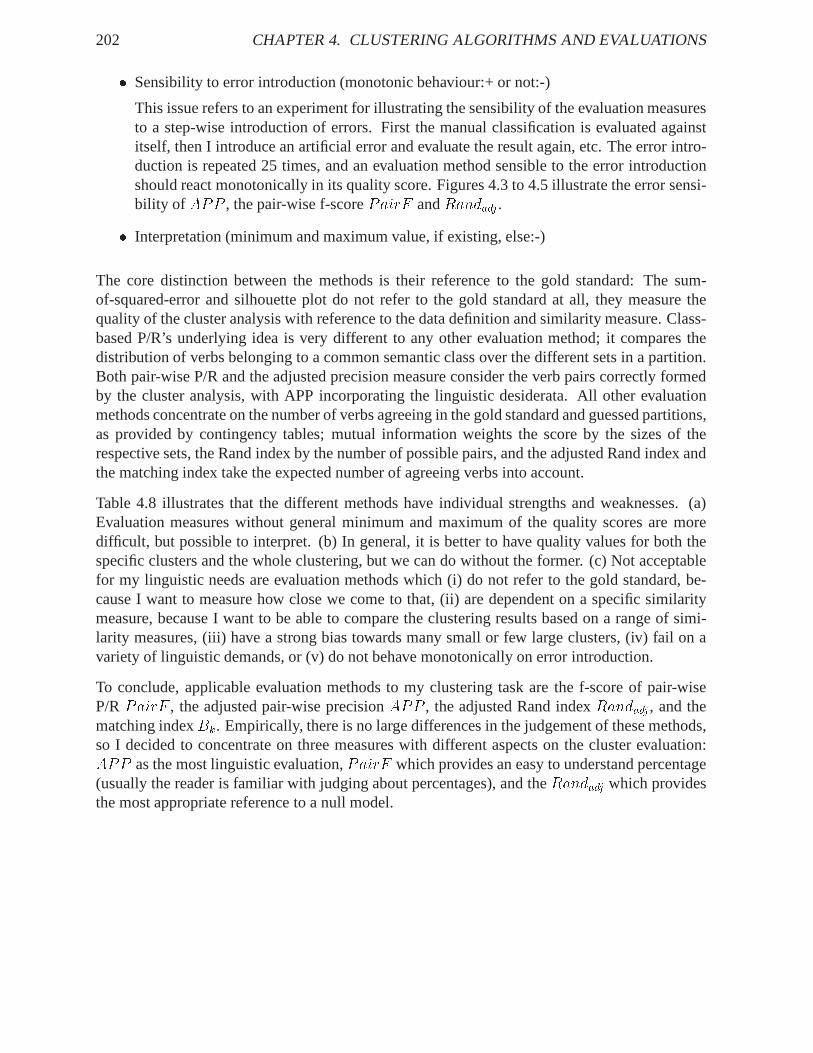
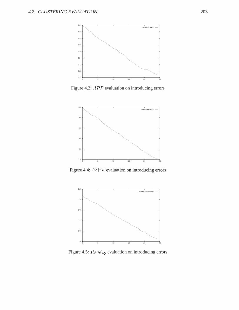
202 CHAPTER 4. CLUSTERING ALGORITHMS AND EVALUATIONS� Sensibility to error introduction (monotonic behaviour:+or not:-)

This issue refers to an experiment for illustrating the sensibility of the evaluation measuresto a step-wise introduction of errors. First the manual classification is evaluated againstitself, then I introduce an artificial error and evaluate theresult again, etc. The error intro-duction is repeated 25 times, and an evaluation method sensible to the error introductionshould react monotonically in its quality score. Figures 4.3 to 4.5 illustrate the error sensi-bility of APP , the pair-wise f-scorePairF andRandadj.� Interpretation (minimum and maximum value, if existing, else:-)

The core distinction between the methods is their referenceto the gold standard: The sum-of-squared-error and silhouette plot do not refer to the gold standard at all, they measure thequality of the cluster analysis with reference to the data definition and similarity measure. Class-based P/R’s underlying idea is very different to any other evaluation method; it compares thedistribution of verbs belonging to a common semantic class over the different sets in a partition.Both pair-wise P/R and the adjusted precision measure consider the verb pairs correctly formedby the cluster analysis, with APP incorporating the linguistic desiderata. All other evaluationmethods concentrate on the number of verbs agreeing in the gold standard and guessed partitions,as provided by contingency tables; mutual information weights the score by the sizes of therespective sets, the Rand index by the number of possible pairs, and the adjusted Rand index andthe matching index take the expected number of agreeing verbs into account.

Table 4.8 illustrates that the different methods have individual strengths and weaknesses. (a)Evaluation measures without general minimum and maximum ofthe quality scores are moredifficult, but possible to interpret. (b) In general, it is better to have quality values for both thespecific clusters and the whole clustering, but we can do without the former. (c) Not acceptablefor my linguistic needs are evaluation methods which (i) do not refer to the gold standard, be-cause I want to measure how close we come to that, (ii) are dependent on a specific similaritymeasure, because I want to be able to compare the clustering results based on a range of simi-larity measures, (iii) have a strong bias towards many smallor few large clusters, (iv) fail on avariety of linguistic demands, or (v) do not behave monotonically on error introduction.

To conclude, applicable evaluation methods to my clustering task are the f-score of pair-wiseP/RPairF , the adjusted pair-wise precisionAPP , the adjusted Rand indexRandadj , and thematching indexBk. Empirically, there is no large differences in the judgement of these methods,so I decided to concentrate on three measures with differentaspects on the cluster evaluation:APP as the most linguistic evaluation,PairF which provides an easy to understand percentage(usually the reader is familiar with judging about percentages), and theRandadj which providesthe most appropriate reference to a null model.


0.21

0.22

0.23

0.24

0.25

0.26

0.27

0.28

0.29

0 5 10 15 20 25

’behaviour-APP’

Figure 4.3:APP evaluation on introducing errors

75

80

85

90

95

100

0 5 10 15 20 25

’behaviour-pairF’

Figure 4.4:PairF evaluation on introducing errors

0.6

0.65

0.7

0.75

0.8

0.85

0 5 10 15 20 25

’behaviour-RandAdj’

Figure 4.5:Randadj evaluation on introducing errors


gold standard similarity measure valueapplicable independent specific whole

Error - + - + +Silhouette - + - + +

ClassR + + + - +ClassP + + + + +ClassF + + + - +

PairR + + + - +PairP + + + - +PairF + + + - +

APP + + + + +MI + + + + +

Rand + + + - +Randadj + + + - +

B-k + + + - +

bias linguistics error interpretation(failure) min max

Error many small b, c, f - - -Silhouette many small b, f - -1 1

ClassR few large a, d, g + 0 100ClassP many small b, f + 0 100ClassF few large a + 0 100

PairR few large a, d, g + 0 100PairP - c, f + 0 100PairF - - + 0 100

APP - - + 0 -MI many small b + 0 -

Rand many small b, d + 0 1Randadj - - + 0 1

B-k - - + 0 1

Table 4.8: Comparison of evaluation measures

4.3. SUMMARY 205

4.3 Summary

This chapter has provided an overview of clustering algorithms and evaluation methods whichare relevant for the natural language clustering task of clustering verbs into semantic classes. Ihave introduced the reader into the background of clustering theory and step-wise related thetheoretical parameters for a cluster analysis to the linguistic cluster demands:� The data objects in the clustering experiments are German verbs.� The clustering purpose is to find a linguistically appropriate semantic classification of the

verbs.� I consider the alternation behaviour a key component for verb classes as defined in Chap-ter 2. The verbs are described on three levels at the syntax-semantic interface, and therepresentation of the verbs is realised by vectors which describe the verbs by distributionsover their features.� As a means for comparing the distributional verb vectors, I have presented a range of sim-ilarity measures which are commonly used for calculating the similarity of distributionalobjects.� I have described a range of clustering techniques and arguedfor applying the hard cluster-ing technique k-Means to the German verb data. k-Means will be used in the clusteringexperiments, initialised by random and hierarchically pre-processed cluster input.� Based on a series of general evaluation demands, general clustering demands and specificlinguistic clustering demands, I have presented a variety of evaluation measures from di-verse areas. The different measures were compared against each other and according to thedemands, and the adjusted pair-wise precisionAPP , the f-score of pair-wise P/RPairF ,and the adjusted Rand indexRandadj were determined for evaluating the clustering exper-iments in the following chapter.

Documents

Chapter 4 Clustering Algorithms and Evaluations · Clustering Algorithms and Evaluations There is a huge number of clustering algorithms and also numerous possibilities for evaluating