Chapter-4

Neural Networks: Algorithms and Methods

May 20, 2009

2

Chapter 1

First-Order Methods for

Learning

An important parameter of neural networks is their connection weights. Fora given architecture, the functionality of a neural network is greatly depen-dent on the values of its weights. We showed a neural network with thevalues of its weights for solving the X-OR problem (Fig. ). Those valueswere hand customized. Such an approach for obtaining the values of weightsis feasible only when neural networks have a small number of connectionsand we can easily map the input-output relationship of a given learningproblem. However, the effort needed for obtaining the correct combinationof weights will be increased substantially for networks with many connec-tions or when the input-output relationships of learning problems can notbe easily mapped. Generally neural networks with many connections arenecessary for solving real-world problems. Le Cun et al. employed a neuralnetwork for recognizing hand written zip codes (digits) provided by the U.S.postal service. The network had on about 98,442 connections and 10 outputneurons, one for each of 10 different digits (0 to 9). The input-output rela-tionship of this recognition can not be easily mapped like the X-OR problemwhere each input pattern is mapped one of two classes. This example givesan impression for obtaining the values of weights automatically so that wecan employ neural networks for solving real-world problems.

Learning is one way for automatically obtaining the values of weights forneural networks. We introduced different learning paradigms in the previous

3

4

chapter. Supervised learning is one paradigm that has attracted an immenseinterest in the neural network community. In this chapter, we shall introducelearning algorithms based on the notion of supervised learning for obtainingthe weights’ value of feedforward and feedback neural networks. In order toshow the essence of learning, we shall first describe a way for obtaining thevalues of weights by an analytical method, which is applicable for obtainingthe weights’ value for a restricted class of network architecture. We shallthen formulate learning as iterative procedure and describe two algorithms.One of these algorithms can be applied to obtain the values of weights for awide range of network architectures.

1.1 Pseudo-Inverse Method

A learning algorithm works iteratively for obtaining the values of weights forneural networks. However, if a neural network has only one set of weights, itmay possible to find the values of its weights directly. An analytical methodto obtain the values of weights of such networks is called the “pseudoinverse”method. In mathematics, the pseudoinverse of a matrix is generalization ofthe inverse matrix, which has some properties of the inverse matrix butnot necessarily all of them. The term pseudoinverse commonly means theMoore-Penrose pseudoinverse, which was independently described by E. H.Moore in 1920 and Roger Penrosein 1955.

We have already seen from chapter 2 that single layered feedforward andRBF networks have only one set of weights. The pseudoinverse methodcan be used for obtaining the values of weights for such networks. Assume aregressing problem is represented by a set of input-output pairs, D = (X,T).We like to obtain the weights’ values of a single layered feedforward or RBFnetwork for solving this regressing problem. At first, we need to construct atraining set by taking input-output pairs from D. Let Dt ⊂ D is a trainingset, which we construct by taking N input-output pairs from D. Since thelearning task is to solve a regression problem, the activation function for theoutput units of the network will be linear. The sum-of-squares error of sucha network is

Neural Networks: Algorithms and Methods 5

E (w) =12

N∑n=1

m∑k=1

((tnk − ynk )2

=12

N∑n=1

m∑k=1

d∑

j=0

wkjxnj − tnk

2

(1.1)

We may consider the learning problem is solved if the outputs of thenetwork yn

k for xn is very much similar to the corresponding target outputstnk for all k and all n. This means the values of weights should be chosen insuch way that they minimize (1.1). It is well known from basic calculus thatthe values of weights minimizes (1.1) when the derivative of (1.1) becomeszero. Thus the necessary and sufficient condition is

∇E (w) =N∑

n=1

m∑

j′=0

wkj′xpj′ − tpk

xpj = 0 (1.2)

To find a solution of (1.2) it is convenient to write it in matrix notation.This gives (1.2) in the following form

(XTX)WT = XTT (1.3)

Here X is a N × d dimensional matrix, W is a m × d dimensional matrixand T is a N ×m dimensional matrix It is evident from (1.3) that if X isnon-singular, the inversion of X, will give a solution of W. This can bewritten in the following form

WT = X†T (1.4)

where X† is a d×N matrix known as the pseudo-inverse of X. This matrixcan be expressed as

X† = (XTX)−1XT (1.5)

6

Although the expression (1.5) gives an exact solution for the values ofweights for single layered or RBF networks, it is not always used in practicefor the following reasons. Firstly, the computational burden of inversinga matrix increases enormously when its dimension increases or when it isnecessary to calculate X† again and again due to changing of X. Secondly,the solution obtained using (1.5) is dependent on two conditions: one isthe non-singularity of X and one is the linearity of output units. Theserestrictions hinder the utilization of neural networks in a wide range ofproblems. Third, we can use use (1.5) when a neural network has only oneset of adjustable weights. We have already discussed in section that MLPnetworks consisted two sets of weights can solve any problem; however, suchnetworks with one one set of weights can not even solve the X-OR problem.Finally, the direct method explicitly program a neural network to performa given task. This approach by-passes one of the unique strengths of neuralnetworks: the ability to program themselves.

1.2 Iterative Method and State Space Search

We have just described various problems associated with the pseudo-inversemethod. Fortunately, we shall be able to avoid most of them by a sim-ple formulation. The problems that we will confront repeatedly are ensur-ing non-singularity in X consisting of training patterns and linearity in theoutput units of a neural network. The avoidance of these constraints willenhance applicability of neural networks with one set of weights. In chap-ter 10, we shall show such networks in a complex domain can solve manylearning problems. The root of the aforementioned two constraints is matrixinversion needed by the pseudo-inverse method. Basic arithmetic operationssuch as multiplications, additions, and subtractions may be good alterna-tives of matrix inversion, since these operations usually do not enforce anyconstraints in computation. Moreover, if the values of weights are found byan iterative method, then such values can be adjusted whenever the inputsor other parameters of a network change. Thus an iterative method with ba-sic arithmetic operations is able to avoid most of the problems encounteredby the pseudo-inverse method.

An iterative method tries to solve a problem by finding successive approx-imations to a solution starting from an initial guess. This method executes


a process involving repeated use of the same formula or step. Typically, theprocess begins with a starting value which is plugged into the formula. Theresult is then taken as the new starting value which is then plugged into theformula again. This process continues to repeat until a termination criterionis satisfied. Iterative methods are usually the only choice for solving non-linear problems. They are, however, often useful even for linear problemsinvolving a large number of variables for which analytic methods (e.g. thepseudo-inverse method) would be prohibitively expensive or in some casesimpossible. From the above discussion, iterative methods can be thought asa search process with four components: the state space, the initial state, thetermination of search (the goal state), and the search strategy. We describethese components in the context of neural networks as follows.

State Space

When using feed-forward or feed-back networks, we must specify the archi-tecture of such networks and the values of their weights. The network archi-tecture, A, can be defined by a set of parameters. These include the numberof neurons, the number of hidden layers in case of feed-forward networks,the activation functions for processing units and the connectivity patternsbetween neurons. We here assume A is fixed and given. We shall describedseveral methods in the chapters 6 and 7 for obtaining A. The goal of thischapter is to describe how we can obtain optimal or near optimal valuesof weights for a given A. Setting this objective, a 2-tuple (A,w) uniquelyspecifies a particular network and its functionality. Note that although twodifferent tuples represent two different networks, the functionality of thesenetworks can be same. This may be easily seen by a simple permutation ofthe weights for the same architecture.

Given a fixed A, a state space S corresponds to the collection of valuesin Rn. A value in Rn represents the value of one weight for a neural network.Iterative methods search S for obtaining a set of optimal or near optimalvalues for the weight matrix W. Each state si ∈ S represents a particularweight vector Wi. This matrix may or may not contain optimal or nearoptimal values for the weights of a neural network.

8

Initial State

A characteristic of iterative methods is that they start from an inital guess,say w0. This w0 is the initial state from which a search process starts. Sincea moderate sized feed-forward or feed-back network has several hundredweights, it is not easy to deterministically assign the values of w0. Alliterative methods used as learning algorithms therefore randomly assign w0.However, an alternative initial state may be used, if prior knowledge of aproblem being solved is available.

Termination of Search (Goal State)

We generally seek solutions of any problem within a finite amount of timeand do not allow infinite amount of time. This is true for easy or complexproblems, although we may allow more time for solving complex problems.The same is true for obtaining the values of weights for neural networks.That is, the search process must somehow be terminated for iterative meth-ods to stop. We have described several stopping criteria in section fromwhich any criterion can be used in the search process for obtaining the valuesof weights. The point in the state space where the search has been stoppedis our goal state.

Search Strategy

Now we come to the crux of search. A search strategy determines howto move from one state to another in the state space, until the search isterminated. Equivalently, the strategy determines how the values of weightsevolve (change) during searching. The search strategy has two essentialparts: one is the search direction and one is the step size. The generalformulation of the search strategy is

wτ+1 = wτ + ητdτ (1.6)

where wτ and wτ+1 are the state at the τ -th (current) and (τ + 1)-th (next)iterations, respectively. The parameter dτ defines the search direction alongwhich the search proceeds from the current state wτ to the next state wτ+1.The amount of movement along dτ is defined by another parameter ητ ,called the step size. The parameter ητ is often called the learning rate in


the context of learning algorithms. Learning rate is specified by the users,which constrains the size of the values of weights changes.

The proper choice of dτ and ητ are very important because it affects con-vergence and solution quality. If dτ is not chosen properly, a search strategymay unable to find appropriate values for weights even after spending manyiterations. The choice of ητ also has a profound influence. We have an op-tion of either taking a very small value for ητ or a large value. If we have anappropriate direction, a very small value for ητ results in a laborious methodof reaching towards the goal state, whereas a very large value may resultin a more zigzag path towards the goal state. We shall describe this issuelatter with respect to a learning algorithm.

1.2.1 Batch and Stochastic Modes of Training

Applications of iterative methods as learning algorithms for training neu-ral networks can be divided in two categories: batch (also called off-line)learning and stochastic (also called on-line) learning. Batch learning is aclassical approach in training a neural network. In this mode of learning,the values of weights for the neural network are only updated (modified)after a complete sweep through the training set. This learning mode can beexpressed as follows:

1. Initialize the weights.

2. Repeat the following steps:

(a) Process all the training data.

(b) Update the weights.

In the above sketch, the exact meaning of “Process” depends on a particularlearning algorithm used for updating the values of weights. We have alreadyseen two important components of updating weights are: the search directionand the step size. The process in this case is deciding the search direction,the step size, or any other parameters necessary for updating the valuesof weights. Batch learning is consistent with the theory of unconstrainedoptimization, since the information from all the training set is used. It canbe viewed as the minimization of an objective function, say E (w). That is,to find the minimizer w∗ = (w∗

1, w∗2, · · · , w∗

n) ∈ Rn, such that:

10

w∗ = minw∈Rn

E (w) (1.7)

where E (w) is the error of a feed-forward or feed-back neural network forall patterns in the training set.

On the other hand, in stochastic learning, the network weights are up-dated after the presentation of each training pattern, which may be sampledwith or without repetition. This corresponds to the minimization of En (w),the network error for a particular training pattern n. Stochastic learningcan be expressed as follows:

1. Initialize the weights.

2. Repeat the following steps

(a) Repeat the following steps for n = 1 to N :

i. Process one training patternii. Update the weights.

It is now understood that the only difference between batch and stochasticlearnings is the number of times the values of weights is updated in an it-eration. The values of weights are updated only once in each iteration ofbatch learning, while these values are updated for N times in each iterationof stochastic learning. When the update of values is computation inten-sive, batch learning may take less time in obtaining the values of weightsfor a neural network. Another advantage of batch learning over stochasticlearning is that most advanced optimization methods, e.g. conjugate gradi-ent and Newton methods, rely on a fixed error surface. This criterion wellsuited for batch learning. However, stochastic learning has several advan-tages over batch learning. Stochastic learning seems more robust becauseerrors, omissions or redundant data in the training set can be easily cor-rected or ejected during training of a neural network. Additionally, trainingdata can often be generated easily and in great quantities when the systemis in operation, whereas such data are usually scarce and precious beforethe operation. Finally, stochastic learning is necessary to learn time varyingfunctions and to continuously update the values of weights in a changingenvironment. In a broad sense, stochastic learning is essential if we want toobtain learning systems as opposed to merely learned ones, as pointed outin [24]


1.3 Error-Correction Learning

We are about to describe the first learning algorithm of this book. Thiserror correcting learning, an iterative method that uses basic arithmeticoperations for updating the values of weights. As the name suggest, thislearning algorithm tries to correct the error of a neural network by iterativelyupdating its weights. Error correction learning was proposed by Widrow andHoff and had been named the Widrow-Hoff rule by Sutton and Barto ().

Let a neuron receives signals a though its weights wτ at any time τ , moreprecisely, the time step of an iterative process. Assume this neuron producesan output y due to the application of a through wτ . The Widrow-Hoff rulefirst compares y with its target output t and computes the error

e(wτ ) = t− y (1.8)

This learning rule then adjusts the values of weights with the aim of briningy closer to t so that the error e(wτ ) reduces. This process continues untila termination criterion has been reached. The actual learning process doesnot take place before the calculation of error is completed, and updatingof the values for weights is made. According to the Widrow-Hoff rule, theadjustment made to wτ is proportional to the product of the error and inputsignals. We thus have

∆wτ ∝ e (wτ )a

= ηe (wτ )a (1.9)

where η is a proportionality constant known as the learning rate. The newweight vector wτ+1 from which the next iteration starts is

wτ+1 = wτ + ηe (wτ )a (1.10)

It is now clear that the Widrow-Hoff rule employs simple arithmeticoperations to adjust the values of weights. This learning rule is also calleddelta rule because the amount of learning is proportional to the difference(or delta) between the target output and the actual output. Since the deltarule does not impose any restriction on the activation function of the unit,

12

this rule can be thought as a generalization of the perceptron learning rulefor which the famous perceptron convergence theorem has been proved. Thelearning rate in (1.9) is equivalent to the search step size and is set by theusers. As mentioned before, in addition to the step size, another importantparameter of the search is direction. It is evident from (1.9) that the deltarule does not employ any optimal search direction; rather, the direction ofa (input vector) specifies the direction of search. Consequently, there is noguarantee that the error will reduce in every iteration of the search.

The Widrow-Hoff rule presumes that the error is directly measurable.Hence, for this measurement to be feasible, we need a supply of desiredresponse from some external source, which must be accessible to the neuron.If the neuron is an output neuron, it is possible of satisfying the abovementioned two conditions provided that a learning problem being solved isrepresented a set of input-output pairs, D = (xn, tn)N

n=1. What will happenif the neuron is a hidden neuron? Certainly, it is not possible to compute theerror for hidden neurons due to the unavailability of exact outputs for suchneurons, and the Widrow-Hoff rule does not give an idea how to computethe error of hidden neurons from the input-output pairs. This bottleneckrestricts the application of the Widrow-Hoff rule for obtaining the values ofweights for feed-forward and feed-back networks with one set of adjustableweights.

Algorithm 1 Widrow-Hoff (X, T, d, m)begin initialize W, η, n← 0, τ ← 1

while (Q 6= ∅) don← n + 1xn ← randomly chosen patternW←W + ηexn

while (n = N) don← 0; τ ← τ + 1 (increment epoch)

end whileend while

return Wend


Algorithm 2 Batch Widrow-Hoff (X, T, d, m)begin initialize h,W, η, τ ← 1

while (Q 6= ∅) don← 0; ∆W← 0while (n 6= N) do

n← n + 1xn ← select pattern∆W← ∆W + ηexn

end whileW←W + ∆Wτ ← τ + 1(increment epoch)

end while

return Wend

1.4 Back-Propagation Learning Algorithm

We discussed that MLP networks could solve any learning problem witharbitrary accuracy (section), so learning algorithms for such networks are ofspecial interest. A very popular learning algorithm for obtaining the valuesof weights in MLP networks is backpropagation or propagation of error. Thisalgorithm was first described by Paul Werbos in 1974, but it wasn’t until1986, through the work of David E. Rumelhart, Geoffrey E. Hinton andRonald J. Williams, that it gained recognition and led to a “renaissance” inthe field of artificial neural networks. It has been one of the most studiedand used algorithms for neural networks learning ever since.

Backpropagation uses the method of steepest descent, an iterative pro-cedure, for obtaining the values of weights in an MLP network. At eachiteration of backpropagation, the values of weights are modified in such adirection for which the error of the network decreases most rapidly. Thisdirection is the negative gradient of the error function (−∇E(w)) at thecurrent point in the weight space. Backpropagation looks for the minimumof the error function by iteratively modifying the values of weights. Thecombination of such values that minimize the error is considered to be a so-lution of a learning problem. Since Backpropagation requires computationof gradient, we must guarantee the continuity and differentiability of the

14

error function. The magnitude of modification is a constant proportion ofthe magnitude of the gradient. Specifically, back-propagation modifies thevalue of each weight by a constant proportion of the partial derivative of theerror with respect to that weight. This proportion is the learning rate orthe step size as described before. The amount of modification to the valueof a weight is given by

∆wpq = −η∂E

∂wpq(1.11)

where wpq is the value of an weight in any layer of a MLP network. We canwrite (1.11) in vector form

∆w = −η∇E|w (1.12)

where the vector w represents the values of all weights in any layer of theMLP network.

The novelty of (1.11) or (1.12) is the simplicity. Once we have a way tocompute the gradient, it is possible to iteratively modify the values for allweights of the MLP network. We may then expect to find a minimum of theerror function, where the gradient vanishes (∇E(w) = 0) or nearly vanishes(∇E(w) = ε). This iterative procedure any iteration τ takes a weight vectorand modifies it in the form

wτ+1 = wτ − η∇E|wτ (1.13)

or in component form

wpq (τ + 1) = wpq (τ)− η∂E

∂wpq(1.14)

To describe the above modification rule elaborately, assume a MLP networkis consisting of an input layer, a hidden layer and an output layer. Thisnetwork has two sets of adjustable weights: one set is the hidden-to-outputweights and one set is the input-to-hidden weights. Let the training set of alearning problem being solved is represented by a set of input-target pairs


(xn, tn)Nn=1. We like to obtain the weights’ values of the MLP network so

that it would able to solve the problem. The backpropagation learning algo-rithm first initializes the weights of the MLP network with random values.The algorithm then iteratively modifies the values of weights until a termi-nation criterion has been met. We shall first consider the way of modifyingthe values of weights that connect the units of the hidden layer to the unitsof the output layer.

Modification of Hidden-to-Output Weights

It is evident from (1.13) that we need to know the error of the MLP tomodify the value of its weights. Since the output units of the MLP networkare “visible” to the outside world and the target values (tn) of these unitsare also given, we measure the error of these units. This error is actuallythe error of the MLP network measured at its output units. For a particulartraining pattern xn, the error En (w) takes the form

En (w) =12

m∑k=1

(tnk − znk )2 (1.15)

where m is the number of units in the output layer. Our objective here isto compute partial derivatives with respect to the hidden-to-output weightsso that we able to use (1.11) for obtaining the amount of modificationsneeded for the values of such weights. Since the error is not explicitly de-pendent upon hidden-to-output weights wkj , we must use chain rule forpartial derivatives:

∂En

∂wkj=

∂En

∂netk

∂netk∂wkj

(1.16)

The first part of the right-hand side in (1.16) describes how the overallerror (not the error of a particular unit) changes with the net activation of anoutput particular unit, for example, here the output unit k, while the secondpart describes how much changing wkj changes the net activation of the unitk. Let the activation function f (·) of the output units is differentiable. Thusthe first part gives

16

∂En

∂netk=

∂En

∂zk

∂zk

∂netk

= − (tnk − zk)∂f (netk)

∂netk= − (tnk − zk) f ′ (netk)

= −δ(2)k (1.17)

where we have defined the quantity

δ(2)k = − (tnk − zk) f ′ (netk) (1.18)

Using (), the second part of (1.16) is found:

∂netk∂wkj

= yj (1.19)

Substituting these results in (1.11), we get the amount of modifications forthe hidden-to-output weights:

∆wkj = −η∂En

∂wkj= ηδ

(2)k yj = η (tnk − yn

k ) f ′ (netk) yj (1.20)

When f (·) is an identity function, we obtain f (netk) = netk and f ′ (netk) =1. The weight modification given by (1.20) for this case is same as thestandard delta rule we saw in the previous section.

Modification of Input-to-Hidden Weights

The modification rule for the input-to-hidden weights wji is more subtlethan that of the hidden-to-output weights wkj . This is because the errorhas direct relation with wkj through the actual outputs yn

k of the outputunits. To formulate the modification rule for wji, we again apply the chainrule to obtain the partial derivative E (w) with respect to wji. This gives

∂En

∂wji=

∂En

∂yj

∂yj

∂netj

∂netj∂wji

(1.21)


The first partial derivative on the right-hand side of (1.21) can be writtenin the form

∂En

∂yj=

∂

∂yj

[12

m∑k=1

(tnk − yk)2

]

= −m∑

k=1

(tnk − yk)∂yk

∂yj

= −m∑

k=1

(tnk − yk)∂yk

∂netk

∂netk∂yj

= −m∑

k=1

(tnk − yk) f ′ (netk) wkj

= −m∑

k=1

δ(2)k wkj (1.22)

Unlike the first partial derivative, the second partial derivative on the right-hand side of (1.21) is obtained without applying any chain rule. Using (),we obtain

∂yj

∂netj=

∂f(netj)∂netj

= f ′ (netj) (1.23)

The third partial derivative on the right-hand side of (1.21) can also beobtained easily. This partial derivative becomes

∂netj∂wji

= xi (1.24)

where we have use (). Plugging all these results into (1.21) we then obtain

∂En

∂wji= −

[m∑

k=1

δkwkj

]f ′ (netj) xi (1.25)

In analogy with (1.17), we define the sensitivity (equivalent to error) of ahidden unit:

δ(1)j = −f ′ (netj)

m∑k=1

δkwkj (1.26)

18

The above expression tells that the sensitivity of a hidden unit is simply thesum of individual errors δks at the output units weighted by the hidden-to-output weights wkj and all multiplied by f ′ (netj). The essence of back-propagation is made it possible for computing the sensitivity of a hiddenunit. Using all these results in (1.12), the amount of modifications we applyto the input-to-hidden weights takes the form

∆wji = −η∂En

∂wji= ηδ

(1)j xi = η

[m∑

k=1

δkwkj

]f ′ (netj) xi (1.27)

It is now evident that we have “propagated back” the errors δ1 · · · δm fromthe output layer to the hidden layer for modifying the values of the input-to-hidden weights. This is why the algorithm is so called “backpropagation” ormore specifically “backpropagation of errors”. The amount of modificationsgiven by (1.20) and (1.27) is similar to the one given by (1.9). The back-propagation learning algorithm is therefore considered as a generalization ofthe delta rule.

Our formulation for modifying the values of weights are essentially amode of stochastic learning, since we use the network error En (w) for aparticular input pattern xn. Hence, in each iteration of stochastic back-propagation, the weights’ values of the network are modified N times for atraining set consisting of N patterns. In the batch mode of backpropagationlearning, we proceed in same way as before. The only exception is that theweights are modified only after the presentation of all N training patterns.Hence it is natural to use the average error Eav(w) over N training patterns,which can be expressed as

Eav(w) =1N

N∑n=1

En(w) =1

2N

N∑n=1

m∑k=1

(tnk − ynk )2 (1.28)

In analogy with (1.20) and (1.27), we obtain the following expressions forthe batch mode of backpropagation

∆wkj = −η∂Eav

∂wkj=−η

N

N∑n=1

∂En

∂wkj=

η

N

N∑n=1

δ(2)k yj (1.29)


∆wji = −η∂Eav

∂wji=−η

N

N∑n=1

∂En

∂wji=

η

N

N∑n=1

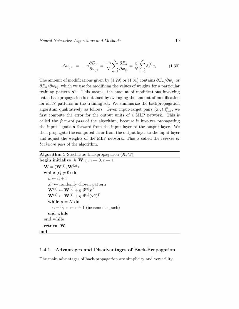
δ(1)j xi (1.30)

The amount of modifications given by (1.29) or (1.31) contains ∂En/∂wji or∂En/∂wkj , which we use for modifying the values of weights for a particulartraining pattern xn. This means, the amount of modifications involvingbatch backpropagation is obtained by averaging the amount of modificationfor all N patterns in the training set. We summarize the backpropagationalgorithm qualitatively as follows. Given input-target pairs (xi, ti)

ni=1, we

first compute the error for the output units of a MLP network. This iscalled the forward pass of the algorithm, because it involves propagatingthe input signals x forward from the input layer to the output layer. Wethen propagate the computed error from the output layer to the input layerand adjust the weights of the MLP network. This is called the reverse orbackward pass of the algorithm.

Algorithm 3 Stochastic Backpropagation (X, T)begin initialize h,W, η, n← 0, τ ← 1

W = (W(1),W(2))while (Q 6= ∅) do

n← n + 1xn ← randomly chosen patternW(2) ←W(2) + η δ(2)yT

W(1) ←W(1) + η δ(1)(xn)T

while n = N don = 0; τ ← τ + 1 (increment epoch)

end whileend while

return Wend

1.4.1 Advantages and Disadvantages of Back-Propagation

The main advantages of back-propagation are simplicity and versatility.

20

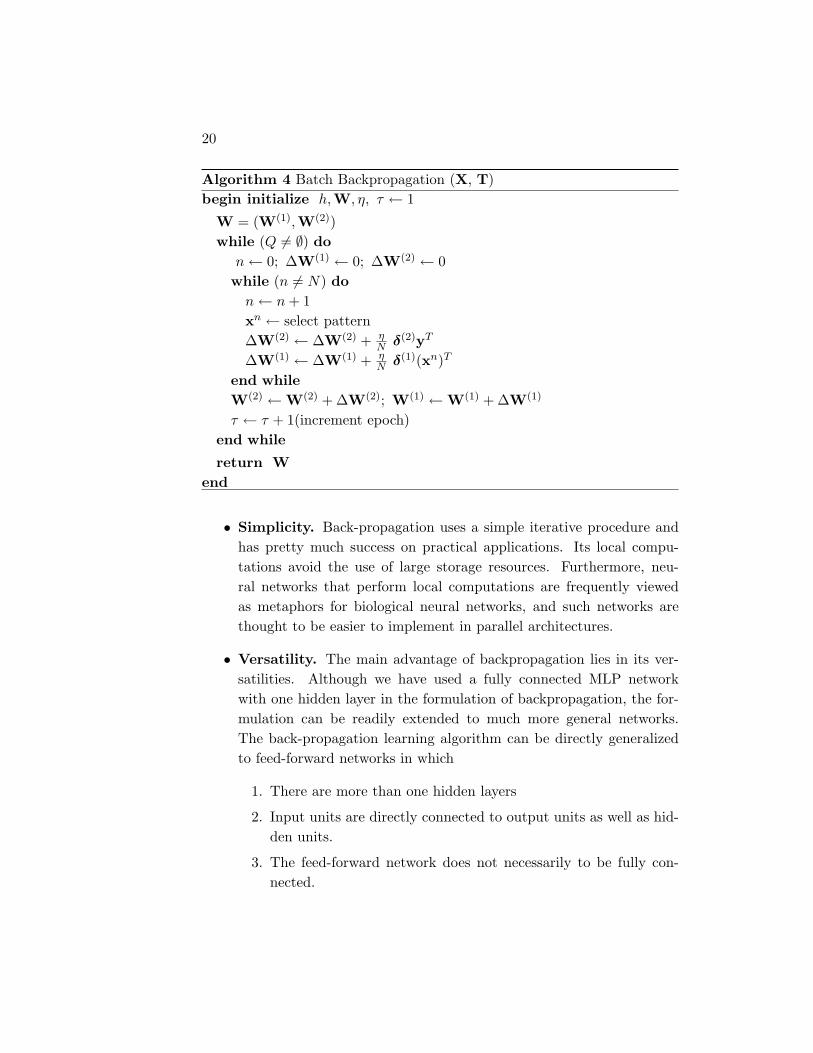
Algorithm 4 Batch Backpropagation (X, T)begin initialize h,W, η, τ ← 1

W = (W(1),W(2))while (Q 6= ∅) do

n← 0; ∆W(1) ← 0; ∆W(2) ← 0while (n 6= N) do

n← n + 1xn ← select pattern∆W(2) ← ∆W(2) + η

N δ(2)yT

∆W(1) ← ∆W(1) + ηN δ(1)(xn)T

end whileW(2) ←W(2) + ∆W(2); W(1) ←W(1) + ∆W(1)

τ ← τ + 1(increment epoch)end while

return Wend

• Simplicity. Back-propagation uses a simple iterative procedure andhas pretty much success on practical applications. Its local compu-tations avoid the use of large storage resources. Furthermore, neu-ral networks that perform local computations are frequently viewedas metaphors for biological neural networks, and such networks arethought to be easier to implement in parallel architectures.

• Versatility. The main advantage of backpropagation lies in its ver-satilities. Although we have used a fully connected MLP networkwith one hidden layer in the formulation of backpropagation, the for-mulation can be readily extended to much more general networks.The back-propagation learning algorithm can be directly generalizedto feed-forward networks in which

1. There are more than one hidden layers

2. Input units are directly connected to output units as well as hid-den units.

3. The feed-forward network does not necessarily to be fully con-nected.


4. Each layer consisting of processing units may use a different ac-tivation function.

5. Each processing units of a layer may may use a different activationfunction.

6. Each connection weights may employ a different learning rate forits modification.

• Computational Efficiency. One of the most important aspects ofbackpropagation is its computational efficiency. Let W be the totalnumber weights (including biases). Both the forward and the back-ward propagation phases require O (W ) operations. We also requireto evaluate W derivatives, one for modifying the values of each weight.The evaluation of derivatives also requires O (W ) operations. Thus thetotal computational cost of backpropagation becomes O (W ), which islinear with respect to the number of weights, that is, to the size of anetwork architecture.

While backpropagation has many desirable properties, it has a number ofproblems as well. These include

• Weight Initialization. The solution quality and convergence speedof backpropagation are dependent on the initial values for the weightsof a network. We shall describe this issue at length and its solution inthe next section.

• Slow Convergence. Backpropagation is slow to converge to a goodsolution in many cases. There are at least two reasons for the slowrate of convergence. Firstly, the magnitude of ∂En/∂wpq or ∂Eav/∂wpq

may be such that the modification of wpq by a constant proportion (afixed η) of that partial derivative will yield a minor reduction in theerror measure. This situation may occur where the error surface isfairly flat along a weight dimension. The magnitude of the partialderivative in this case will be small. This leads to a small amount ofmodification for that particular weight. Thus many iterations will benecessary to reduce error significantly. Alternatively, where the errorsurface is highly curved along a weight dimension, the derivative ofthe weight is large in magnitude. Thus, the value of the weight will

22

be modified by a large amount and it may overshoot the minimumof the error surface along that weight dimension. Secondly, we haveseen from (1.20) or (1.27) the derivative of a unit’s output appears(f ′ (net)) for modifying the input weights of that unit. This derivativeis zero or nearly zero in the extremes of f (·) used to compute the unit’soutput. Weights will be not modified when such a situation happeneven though modifications are necessary for reducing error. We shalldescribe some methods in the next chapter to

• Local Optima. A common problem of the gradient descent methodas other hill-climbing methods is that the search process may at lo-cal optima- a state where no small modification of the weights valuewill produce a better solution (e.g. less error) than the current solu-tion. Since backpropagation uses a method of gradient descent, thisalgorithm is not free from the local optima problem.

It may not be immediately apparent why only a small step istaken in the direction of the gradient. Could we not move allthe way in this direction and completely eliminate the error onthe example? In many cases this could be done, but usually it isnot desirable. Remember that we do not seek or expect to finda value function that has zero error on all states, but only anapproximation that balances the errors in different states. If wecompletely corrected each example in one step, then we would notfind such a balance. In fact, the convergence results for gradientmethods assume that the step-size parameter decreases over time.If it decreases in such a way as to satisfy the standard stochasticapproximation conditions (2.7), then the gradient-descent method(8.2) is guaranteed to converge to a local optimum.

1.4.2 Heuristics for Efficient Initialization of Weights

While it might seem natural to start backpropagation by initializing thevalues of weights to zero, it is evident from (1.23) that there would be veryundesirable consequences. Let the initial values for the hidden-to-outputweights of a MLP network are set to zero. With these initialization thevalues for the input-to-hidden weights will never change. This situation is


equivalent to “no learning”. Consider a different scenario in which the initialvalues for all weights of the MLP network are set equal. Let the solution ofa given learning problem requires unequal values for the weights. Will back-propagation able to develop such values from equal initial values? This isnever possible because the backpropagation learning algorithm propagatedback the errors computed at the output units through the weights in pro-portion to the values of weights. This means that all hidden units will getidentical error signals. Since the modification to the values of weights de-pends on the error signals, the values for hidden-to-output weights will mustalways be the same. A similar situation will also occur to the values for theinput-to-hidden weights. This problem is called “symmetry” problem. For-tunately, we able to easily counteract no-learning and symmetry problemsby randomly initializing the values for the weights. In backpropagation, werandomly initialize the weights with an small range, for example, -0.5 to+05, -1 to +1 and so. However, the random initialization may cause thesaturation of processing units’ activity resulting in slow convergence.

Consider the MLP network has one hidden layer. The output, op, of anyprocessing (hidden or output) unit pis

op = φ

∑j

wpqaq

= φ(netp) (1.31)

where aq are the input signals to the unit p, wpq are the incoming weightsthat carry the input signals, and φ is the unit’s activation function. Asseen from Fig., an activation function has some active regions where theoutput of a processing unit varies due to variation to the incoming weightsto the unit. It is also seen that there are also some saturation regions wherethe processing unit’s output does not vary due to variation of the incomingweights. The expressions (1.20) and (1.23) indicate that the modificationto the values of weights is dependent on φ′(netp). The derivative evaluatedany point in the saturation region is zero or nearly zero. Accordingly, thevalues of the weights in successive iterations will be remain almost same,even when the error is still large and it is necessary to modify the values ofweights. We have nothing to do with the input signals; hence, for a given φ,the weights are to be initialized in such a way so that the processing unitscan operate in the active regions of φ. Assume φ is a sigmoid function, which

user

Highlight

user

Underline

24

is widely used. The active region of sigmoid, for example, can be consideredbetween 0.1 and 0.9. Let op = yj (j = 1, · · · , h) are the outputs of hiddenneurons. The task now is to assign the initial values for wji (equivalent towpq) so that the outputs of the hidden neurons lies in the above mentionedrange.

To obtain such initial values, we first assign the outputs of hidden unitswith random values in the range between 0.1 and 0.9. Let the matrix T′ ofdimensions N×h denotes the random values for the h hidden units of a MLPnetwork for the input matrix X of dimensions N ×d. We consider T′ as thetarget values for the hidden units. The task now is to obtain the values forthe input-to-hidden weights so that the actual outputs of hidden units, Y ofdimensions N × h, become very close to T′. This task becomes similar toobtaining values for the weights of a single-layer network, where the hiddenlayer of the MLP network is to be considered as the output layer of the single-layer network. Given a set of input-target pairs (X,T′), the values for theweights of the single-layer network can be obtained using the delta rule. Theobtained values will be the initial values for the input-to-hidden weights ofthe MLP network. In the same way we can obtain the initial values for thehidden-to-output weights. Since the target values for the output units ofthe MLP network are known, it is not necessary to initialize these valuesrandomly. Note that Y will act as inputs for obtaining the values for thehidden-to-output weights. If the activation function of the output units islinear, we may also use the pseudo-inverse method in obtaining the valuesfor the hidden-to-output weights.

1.4.3 Heuristics for Avoiding Local Optima

Figure shows a error surface for only two weights. We can consider thissurface as mountains of terrains. Ideally a gradient descent method seeksthe global minimum, the lowest point in the entire terrain. Judith Dayhoff

1.4.4 Convergence of Backpropagation

Amin Write here convergence issue


1.5 Learning Methods for RBF networks

The RBF network is another class of feed-forward networks capable of solv-ing any learning problem with arbitrary accuracy. Since the free parametersassociated with this networks are the basis function parameters and theweights, the learning methods described so far cannot be directly applied inobtaining the values for all such parameters, specifically the values for thecenters and widths of the basis function. There are two different ways forobtaining the values of the centers, widths, and weights:

1. First obtain the values for the centers and widths and then the valuesfor the weights.

2. Simultaneously obtain the values for the centers, widths and weights.

1.5.1 Case 1

Let the hidden layer of the RBF network is consisting of h units (corre-sponding to h basis functions). One method in obtaining the values for thecenters cj (j = 1, · · · , h) of the basis functions is the random selection. It isusually done by randomly selecting h input vectors (training patterns) fromthe training set. This is the simplest approach and reasonable only if all N

input vectors in the training set are distributed in a representative manner.Typically, the number h is much less than the number N . The widths of thebasis functions can be kept fixed and same, that is, σj = σ (j = 1, · · · , h).This is reasonable in the sense that RBF networks with such a fixed width,even thus restricted, are still universal approximators (Park and Sandberg).The fixed width σ can be set by some heuristic (Moody and Darken). Forthe Gaussian basis function, the width is given by

σ =Dmax√

2h(1.32)

where Dmax is the maximum distance between chosen centers. The aboveformula ensures that the individual radial-basis functions are not too peakedor too flat.

As mentioned before (section), the role of hidden units in the RBF net-work is different with respect to those of the MLP network. The RBF

user

Highlight

26

network with localized basis functions forms representation in the space ofhidden units, which is local with respect to the input space. This is because,for a given input vector, typically few hidden units will have significant acti-vations. Thus the basis functions centers are thought to be as “prototypes”of the input vector. This viewpoint suggests that the centers and widths ofthe basis function should be chosen to form a representation of the inputvectors. This leads to an unsupervised learning procedure, specifically aclustering method, for obtaining the values of the basis functions parame-ters which utilizes only on the input vectors and ignores target vectors. Weshall describe clustering methods in chapter 6.

So far our discussion has been limited to the ways of obtaining the valuesfor the centers and widths of the basis functions. The RBF network usuallyhas one hidden layer, so there is one set of weights that connect the hiddenunits to the output units. The values for these weights can obtained usingthe methods descried earlier. We shall describe the pseudo-inverse methodin the context of the RBF network. Let the output units of the networkare linear, a condition for applying the pseudo-inverse method to obtain thevalues of weights. The error function for the RBF network takes the form

En (w) =12

∑k

(tnk − znk )2 (1.33)

where

znk =

h∑j=1

wkj exp(−h

D2max

‖xn − cj‖2)

(1.34)

The aim of the pseudo-inverse method is to obtain the values of the weightsfor which tnk and zn

k are same for all k and all n. For non-RBF networks,we have already formulated an expression by satisfying the above criterion.The same expression with some notational variation is also applicable forthe RBF network. This variation is due to the fact that the output unitsof RBF networks receive signals from the hidden units not from the inputunits. Thus, we write

W = Y†T (1.35)

user

Highlight


where Y is a N×h dimensional matrix representing the outputs of h hiddenunits for N input vectors. The matrix Y† is the pseudo-inverse of Y, whichis itself defined as

Y = {ynj} (1.36)

where

ynj = exp(−h

D2max

‖xn − cj‖2)

, n = 1, 2, · · · , N ; j = 1, 2, · · · , h (1.37)

Although the pseudo-inverse method can not be applied to the RBF net-work with nonlinear output units, the delta rule and the gradient descentmethod can be applied to such network with linear or nonlinear output units.These two methods obtain the values for weights of the RBF network byusing an iterative procedure, which we have already formulated for the non-RBF network. The same formulation with minor variation is also applicablefor the RBF network. In case of the delta rule, there is notational variationas just we deal with the pseudo-inverse method for the RBF network. Un-like the back-propagation algorithm for the non-RBF (MLP) network, thegradient descent method for the RBF network does not require backwardpropagation of errors. This advantage is due to the one set of weights in theRBF network.

1.5.2 Case 2

The two-stage approach described above is not always a good choice in ob-taining the parameters value of the RBF network. One major disadvantageis that the second-stage of such an approach, if necessary, cannot modifythe outcomes of the first-stage. Furthermore, the second-stage, if necessary,cannot add any hidden units. This is because the first-stage obtains thevalues for centers and width associated with the hidden units. These factssuggest to obtain simultaneously all parameters, (the centers, widths, andweights) value of the RBF network. At this juncture, the gradient descentmethod is a natural choice for such an one-stage approach. We shall de-scribe several learning methods in the next two chapters some of thosemethods are also be chosen.

user

Underline

28

Since we like to obtain the values for the centers and widths in additionto the values for the weights, the arguments of the error function will bethese three parameters. The RBF network with linear outputs is widelyused for regression problems; however, such network with nonlinear outputsis also used for classification problems. Thus we here assume that the outputunits of the RBF network uses an activation f , which can be the identityor nonlinear function. This assumption gives an opportunity to formulategeneral expressions. Considering all these factors we take the error functionto have the form

En (w, c, σ) =12

∑k

(tnk − znk )2 =

12

∑k

e2k (1.38)

where

znk = f (netk) = f

h∑j=1

wkjyj

(1.39)

in which

yj = exp

(−‖x

n − cj‖2σ2

j

)(1.40)

To apply the concept of gradient descent, it is necessary to compute the par-tial derivatives ∂En/∂wkj , ∂En/∂cji and ∂En/∂σj for obtaining the valuesof wkj , cji, and σj . We have already computed ∂En/∂wkj in for the MLPnetwork. The same formulation expressed by () is also applicable for theRBF network. As before, we apply the chain rule to compute ∂En/∂cji. Wetherefore have

∂En/∂cji =∑

k

[∂En

∂znk

∂znk

∂yj

]∂yj

∂cji

=∑

k

[∂En

∂zk

∂znk

∂netk

∂netk∂yj

]∂yj

∂cji(1.41)

Using (1.17), (1.26),(1.39) and (1.40), we obtain


∂En/∂cji = −

[∑k

δ(2)k wkj

]exp

(−‖x

n − cj‖2σ2

j

)(xn

i − cji)σ2

j

= −δ(1)j exp

(−‖x

n − cj‖2σ2

j

)(xn

i − cji)σ2

j

= −δ(1)j y

(c)j (1.42)

where cji denotes the ith component of cj and we have defined the quantity

exp

(−‖x

n − cj‖2σ2

j

)(xn

i − cji)σ2

j

= y(c)j (1.43)

To compute ∂En/σj , we again apply the chain rule and obtain the fol-lowing expression

∂En/∂σ2j =

[∑k

∂En

∂zk

∂zk

∂yj

]∂yj

∂σ2j

=

[∑k

∂En

∂zk

∂zk

∂netk

∂netk∂yj

]∂yj

∂σ2j

(1.44)

Making use of (1.17), (1.38), (1.39) and (1.40), we can write (1.44) in theform

∂En/∂σ2j = −δ

(1)j exp

(−‖x

n − cj‖2σ2

j

)‖xn − cj‖

2σ4j

= −δ(1)j y

(σ)j (1.45)

where

exp

(−‖x

n − cj‖2σ2

j

)‖xn − cj‖

2σ4j

= y(σ)j (1.46)

We are now in position to formulate expressions for modifying the valuesof the weights, centers and widths of the RBF network. The characteristics

30

and tasks of the above mentioned three parameters are different, so it isnatural to use a separate learning for each of these parameters. Let η1, η2

and η3 be the learning rates to modify the values for the weights, centersand widths. Thus the expressions for modifying these values become

wkj (τ + 1) = wkj (τ)− η1∂En

∂wkj

= wkj (τ) + η1δ(2)k yj (1.47)

cji (τ + 1) = cji (τ)− η2∂En

∂cji

= cji (τ) + η2δ(1)j y

(c)j (1.48)

σ2j (τ + 1) = σ2

j (τ)− η3∂En

∂σ2j

= σ2j (τ) + η3δ

(1)j y

(σ)j (1.49)

The above mentioned rules work on the assumption that the initial pa-rameters’ values are provided. We then start searching from the initialvalues and continue until satisfying a given termination criterion. Withouta proper initialization, the modification rules may generate a set of poorfinal values. As before, we also obtain here the initial values for the weightsby randomly assigning them within a small range. However, the initializa-tion of the center and widths are not simple. Specifically, it is necessary toconsider the distribution data for initializing the centers. If the centers areinitialized too far away from the data, the final values of the centers maybe such that they have no association with the data. Thus it is better to(randomly) select the initial centers from the data or to select the initialcenter to some uniform random values within the range of the data. Writehere about the width. Also clustering methods can be used to initializethe centers and widths, after which the initial values ‘fine tuned’ using (1.45)and (1.52). We have described the advantages and disadvantages describedbackpropagation that uses the method of gradient descent, which are alsoapplicable here also. Furthermore, the gradient descent method in the RBFnetwork encounters the locality problem. This is because there is is not guar-antee that the basis function will be remain localized when its centers andwidths are modified by the gradient descent method.


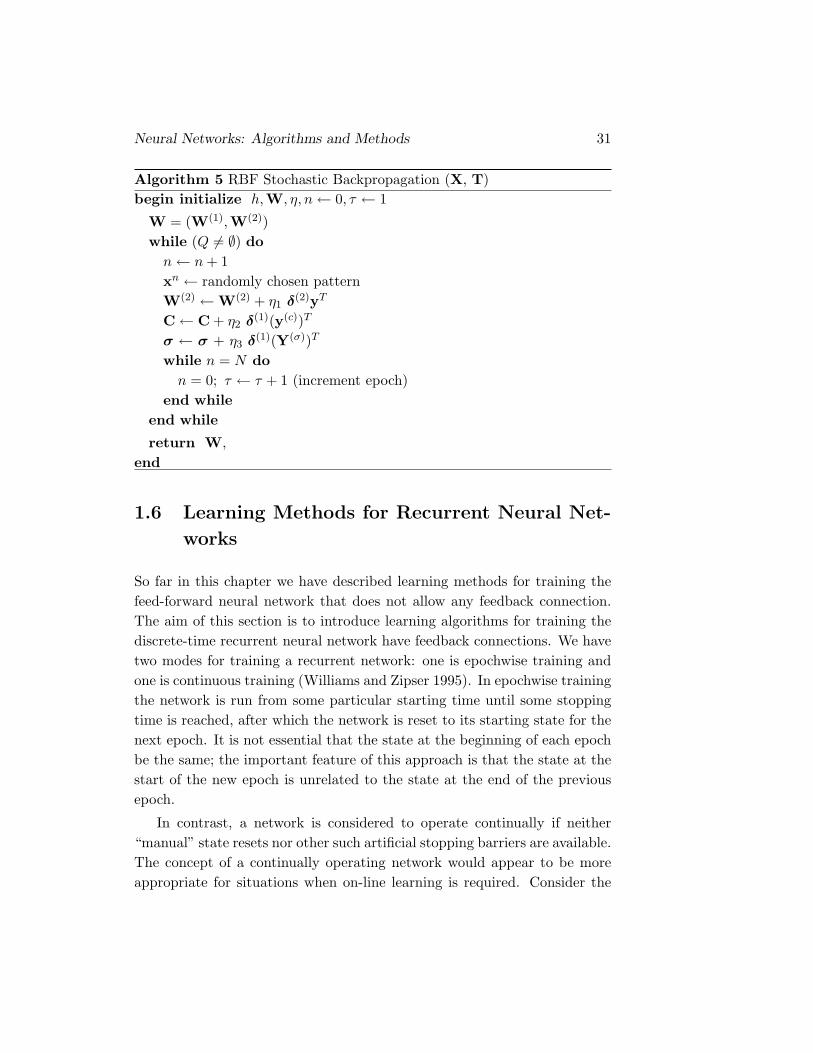
Algorithm 5 RBF Stochastic Backpropagation (X, T)begin initialize h,W, η, n← 0, τ ← 1

W = (W(1),W(2))while (Q 6= ∅) do

n← n + 1xn ← randomly chosen patternW(2) ←W(2) + η1 δ(2)yT

C← C + η2 δ(1)(y(c))T

σ ← σ + η3 δ(1)(Y(σ))T

while n = N don = 0; τ ← τ + 1 (increment epoch)

end whileend while

return W,

end

1.6 Learning Methods for Recurrent Neural Net-

works

So far in this chapter we have described learning methods for training thefeed-forward neural network that does not allow any feedback connection.The aim of this section is to introduce learning algorithms for training thediscrete-time recurrent neural network have feedback connections. We havetwo modes for training a recurrent network: one is epochwise training andone is continuous training (Williams and Zipser 1995). In epochwise trainingthe network is run from some particular starting time until some stoppingtime is reached, after which the network is reset to its starting state for thenext epoch. It is not essential that the state at the beginning of each epochbe the same; the important feature of this approach is that the state at thestart of the new epoch is unrelated to the state at the end of the previousepoch.

In contrast, a network is considered to operate continually if neither“manual” state resets nor other such artificial stopping barriers are available.The concept of a continually operating network would appear to be moreappropriate for situations when on-line learning is required. Consider the

32

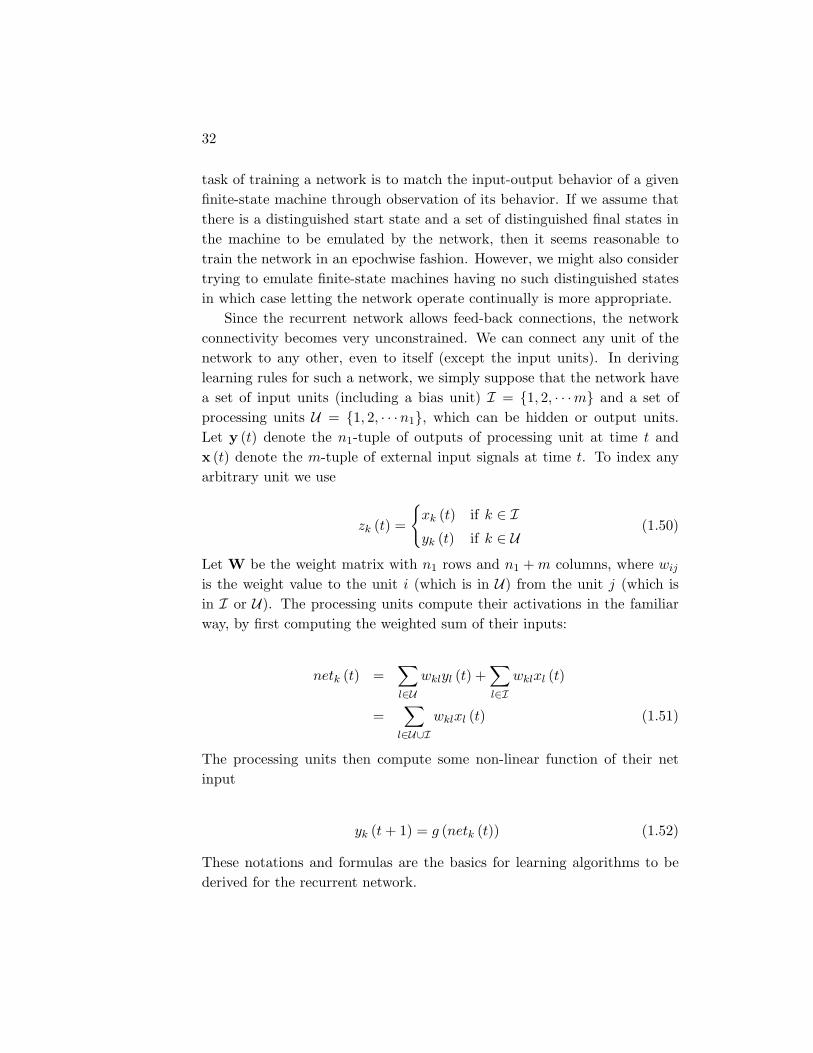
task of training a network is to match the input-output behavior of a givenfinite-state machine through observation of its behavior. If we assume thatthere is a distinguished start state and a set of distinguished final states inthe machine to be emulated by the network, then it seems reasonable totrain the network in an epochwise fashion. However, we might also considertrying to emulate finite-state machines having no such distinguished statesin which case letting the network operate continually is more appropriate.

Since the recurrent network allows feed-back connections, the networkconnectivity becomes very unconstrained. We can connect any unit of thenetwork to any other, even to itself (except the input units). In derivinglearning rules for such a network, we simply suppose that the network havea set of input units (including a bias unit) I = {1, 2, · · ·m} and a set ofprocessing units U = {1, 2, · · ·n1}, which can be hidden or output units.Let y (t) denote the n1-tuple of outputs of processing unit at time t andx (t) denote the m-tuple of external input signals at time t. To index anyarbitrary unit we use

zk (t) =

{xk (t) if k ∈ Iyk (t) if k ∈ U

(1.50)

Let W be the weight matrix with n1 rows and n1 + m columns, where wij

is the weight value to the unit i (which is in U) from the unit j (which isin I or U). The processing units compute their activations in the familiarway, by first computing the weighted sum of their inputs:

netk (t) =∑l∈U

wklyl (t) +∑l∈I

wklxl (t)

=∑

l∈U∪Iwklxl (t) (1.51)

The processing units then compute some non-linear function of their netinput

yk (t + 1) = g (netk (t)) (1.52)

These notations and formulas are the basics for learning algorithms to bederived for the recurrent network.


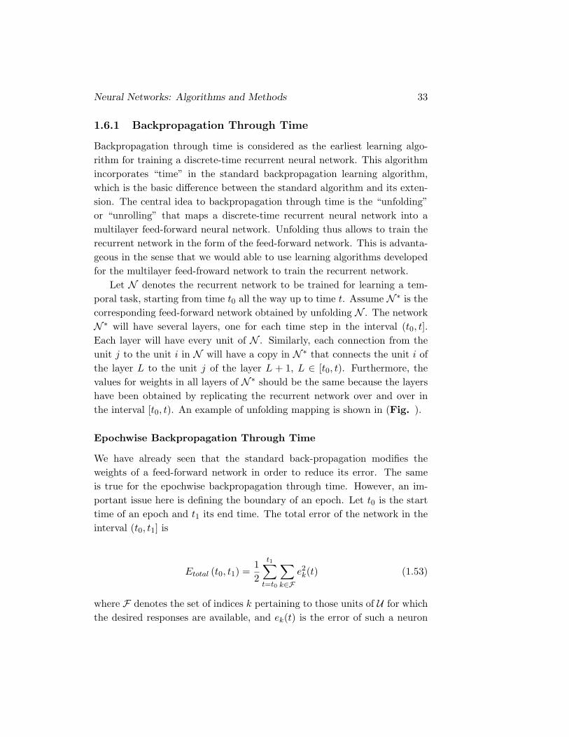
1.6.1 Backpropagation Through Time

Backpropagation through time is considered as the earliest learning algo-rithm for training a discrete-time recurrent neural network. This algorithmincorporates “time” in the standard backpropagation learning algorithm,which is the basic difference between the standard algorithm and its exten-sion. The central idea to backpropagation through time is the “unfolding”or “unrolling” that maps a discrete-time recurrent neural network into amultilayer feed-forward neural network. Unfolding thus allows to train therecurrent network in the form of the feed-forward network. This is advanta-geous in the sense that we would able to use learning algorithms developedfor the multilayer feed-froward network to train the recurrent network.

Let N denotes the recurrent network to be trained for learning a tem-poral task, starting from time t0 all the way up to time t. Assume N ∗ is thecorresponding feed-forward network obtained by unfolding N . The networkN ∗ will have several layers, one for each time step in the interval (t0, t].Each layer will have every unit of N . Similarly, each connection from theunit j to the unit i in N will have a copy in N ∗ that connects the unit i ofthe layer L to the unit j of the layer L + 1, L ∈ [t0, t). Furthermore, thevalues for weights in all layers of N ∗ should be the same because the layershave been obtained by replicating the recurrent network over and over inthe interval [t0, t). An example of unfolding mapping is shown in (Fig. ).

Epochwise Backpropagation Through Time

We have already seen that the standard back-propagation modifies theweights of a feed-forward network in order to reduce its error. The sameis true for the epochwise backpropagation through time. However, an im-portant issue here is defining the boundary of an epoch. Let t0 is the starttime of an epoch and t1 its end time. The total error of the network in theinterval (t0, t1] is

Etotal (t0, t1) =12

t1∑t=t0

∑k∈F

e2k(t) (1.53)

where F denotes the set of indices k pertaining to those units of U for whichthe desired responses are available, and ek(t) is the error of such a neuron

34

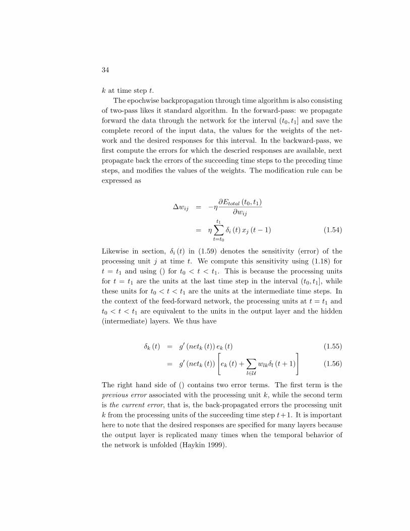
k at time step t.The epochwise backpropagation through time algorithm is also consisting

of two-pass likes it standard algorithm. In the forward-pass: we propagateforward the data through the network for the interval (t0, t1] and save thecomplete record of the input data, the values for the weights of the net-work and the desired responses for this interval. In the backward-pass, wefirst compute the errors for which the descried responses are available, nextpropagate back the errors of the succeeding time steps to the preceding timesteps, and modifies the values of the weights. The modification rule can beexpressed as

∆wij = −η∂Etotal (t0, t1)

∂wij

= η

t1∑t=t0

δi (t) xj (t− 1) (1.54)

Likewise in section, δi (t) in (1.59) denotes the sensitivity (error) of theprocessing unit j at time t. We compute this sensitivity using (1.18) fort = t1 and using () for t0 < t < t1. This is because the processing unitsfor t = t1 are the units at the last time step in the interval (t0, t1], whilethese units for t0 < t < t1 are the units at the intermediate time steps. Inthe context of the feed-forward network, the processing units at t = t1 andt0 < t < t1 are equivalent to the units in the output layer and the hidden(intermediate) layers. We thus have

δk (t) = g′ (netk (t)) ek (t) (1.55)

= g′ (netk (t))

[ek (t) +

∑l∈U

wlkδl (t + 1)

](1.56)

The right hand side of () contains two error terms. The first term is theprevious error associated with the processing unit k, while the second termis the current error, that is, the back-propagated errors the processing unitk from the processing units of the succeeding time step t+1. It is importanthere to note that the desired responses are specified for many layers becausethe output layer is replicated many times when the temporal behavior ofthe network is unfolded (Haykin 1999).


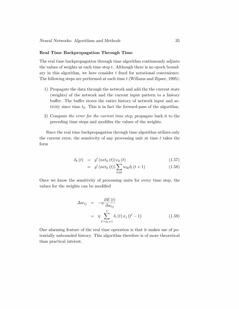
Real Time Backpropagation Through Time

The real time backpropagation through time algorithm continuously adjuststhe values of weights at each time step t. Although there is no epoch bound-ary in this algorithm, we here consider t fixed for notational convenience.The following steps are performed at each time t (Willams and Zipser, 1995):

1) Propagate the data through the network and add the the current state(weights) of the network and the current input pattern to a historybuffer. The buffer stores the entire history of network input and ac-tivity since time t0. This is in fact the forward-pass of the algorithm.

2) Compute the error for the current time step, propagate back it to thepreceding time steps and modifies the values of the weights.

Since the real time backpropagation through time algorithm utilizes onlythe current error, the sensitivity of any processing unit at time t takes theform

δk (t) = g′ (netk (t)) ek (t) (1.57)

= g′ (netk (t))∑l∈U

wlkδl (t + 1) (1.58)

Once we know the sensitivity of processing units for every time step, thevalues for the weights can be modified

∆wij = −η∂E (t)∂wij

= ηt∑

t′=t0+1

δi (t) xj

(t′ − 1

)(1.59)

One alarming feature of the real time operation is that it makes use of po-tentially unbounded history. This algorithm therefore is of more theoreticalthan practical interest.

Documents

Chapter-4