Embed Size (px)
Citation preview
Chapter 3
Voting Systems
3.1 Introduction
We rank everything. We rank movies, bands, songs, racing cars, politicians, professors, sports
teams, the plays of the day. We want to know “who’s number one?” and who isn’t. As a lo-
cal sports writer put it, “Rankings don’t mean anything. Coaches continually stress that fact.
They’re right, of course, but nobody listens. You know why, don’t you? People love polls.
They absolutely love ’em” (Woodling, December 24, 2004, p. 3C). Some rankings are just for
fun, but people at the top sometimes stand to make a lot of money. A study of films released
in the late 1970s and 1980s found that, if a film is one of the 5 finalists for the Best Picture
Oscar at the Academy Awards, the publicity generated (on average) generates about $5.5 mil-
lion in additional box office revenue. Winners make, on average, $14.7 million in additional
revenue (Nelson et al., 2001). In today’s inflated dollars, the figures would no doubt be higher.
Actors and directors who are nominated (and who win) should expect to reap rewards as well,
since the producers of new films are eager to hire Oscar-winners.
This chapter is about the procedures that are used to decide who wins and who loses. De-
veloping a ranking can be a tricky business. Political scientists have, for centuries, wrestled
with the problem of collecting votes and moulding an overall ranking. To the surprise of un-
1
CHAPTER 3. VOTING SYSTEMS 2
dergraduate students in both mathematics and political science, mathematical concepts are at
the forefront in the political analysis of voting procedures. Mathematical tools are important in
two ways. First, mathematical principles are put to use in the scoring process that ranks the al-
ternatives. Second, mathematical principles are used to describe the desired properties of a vot-
ing procedure and to measure the strengths and weaknesses of the procedures. Mathematical
concepts allow us to translate important, but vague, ideas like “logical” and “fair” into sharp,
formally defined expressions that can be applied to voting procedures.
In this chapter, we consider a number of example voting procedures and we discuss their
strengths and weaknesses.
3.2 Mathematical concepts
3.2.1 Transitivity.
Real numbers are transitive. Every school child knows that transitivity means that
If x > y and y > z, then x > z (3.1)
The symbol > means “greater than” and ≥ means “greater than or equal to.” Both of these
are transitive binary relations. “Binary” means only two numbers are compared against each
other, and transitivity means that many number can be linked together by the binary chain. For
example, we can work our way through the alphabet. If a > b, and b > c, and ... x > y, then
a > z.
If a , b, and c represent policy proposals or football teams being evaluated, we expect that
voters are able to make binary comparisons, declaring that one alternative is preferred to an-
other, or that they are equally appealing. The parallel between “greater than” and “preferred
to” is so strong, in fact, that we use the symbol � to represent “preferred to.” The subscript i
indicates that we are talking about a particular voter, so x �i y means that voter i prefers x to
CHAPTER 3. VOTING SYSTEMS 3
y and x �i y means that x is as good as y. If i is indifferent, we write x ≈i y.
Using the binary relations �i and �i, it is now possible to write down the idea of transi-
tive preferences. If a person’s preferences are transitive, the following holds:
If x �i y and y �i z, then x �i z (3.2)
This can be written more concisely as
x �i y �i z (3.3)
According to William Riker, a pioneer in the modern mathematical theory of voting, tran-
sitivity is a basic aspect of reasonable human behavior (Riker, 1982). Someone who prefers
green beans to carrots, and also prefers carrots to squash, is expected to prefer green beans to
squash. One of the truly surprising–even paradoxical–problems that we explore in this chap-
ter is that social preferences, as expressed through voting procedures, may not be transitive.
The procedure of majority rule, represented by the letter M , can compare alternatives so that
x �M y, y �M z, and yet x does not defeat z in a majority election. The fact that individu-
als may be transitive, but social decision procedures are not, has been a driving force in voting
research.
3.2.2 Ordinal versus Cardinal Preferences
If x �i y, we know that x is preferred to y, but we don’t know by “how much.” These are
called ordinal preferences because they contain information only about ordering, and not mag-
nitude. Can the magnitude of the difference be measured? The proponents of an alternative
model, called cardinal preferences, have developed ingenious mathematical techniques to mea-
sure preferences.
The proponents of ordinal preferences argue that all of the information about the tastes
of the voters that is worth using is encapsulated in a statement like x �i y. Even if we could

CHAPTER 3. VOTING SYSTEMS 4
measure the gap in the desirability between x and y in the eyes of voter i, it would still not
solve the problem that the gaps observed by voters i and j would not be comparable. There is
no rigorous, mathematically valid way to express the idea that i likes policy x “twice as much”
as voter j, even though such an interpersonal comparison is tempting. As a result, the ordinal-
ists argue that no voting procedure should be designed with the intention of trying to measure
“how much” more attractive x is than y. Only the ranking should be taken into account.
The approaches based on cardinal preferences offer the possibility of very fine-grained
and, at least on the surface, precise social comparisons. If we had a reliable measure of pref-
erences on a cardinal scale, perhaps it would be possible to say that x is .3 units more appeal-
ing than y. The most widely used method of deriving these preferences is the Von Neumann-
Morgenstern approach which is used in game theory (see chapter X). The theory that justifies
the measurement techniques is somewhat abstract and complicated. Even in a laboratory set-
ting, these preferences have proven difficult to measure reliably.
For whatever reasons, almost all voting procedures in use in the world today employ or-
dinal methods. We ask voters to declare their favorite or to rank the alternatives first, sec-
ond, and third. As we discuss the weaknesses of various voting methods, readers will often
be tempted to wonder if the use of cardinal preference information might lead to an easy fix.
We believe that such quick fixes are unlikely to be workable, but they are often very interest-
ing. The fact that one cannot compare preference scores across individual voters should never
be forgotten, because many proposals implicitly assume that such comparisons are meaningful.
3.2 Exercises
1. Consider 3 lunch items, steak, fish, and eggplant. If Joe prefers steak to fish, we write
steak �Joe fish. Joe also prefers fish to eggplant. If Joe’s preferences are transitive,
should we conclude steak �Joe eggplant or eggplant �Joe steak?
2. Suppose Jennifer tells us steak �Jennifer fish and steak �Jennifer eggplant. Can we
say whether steak �Jennifer fish or fish �Jennifer steak?
CHAPTER 3. VOTING SYSTEMS 5
3. If pink �Mary red and red �Mary green, and then Mary says she prefers green to pink,
would her choices seem reasonable to you? Why?
3.3 The Plurality Problem
By far the most commonly used election procedure in the United States is simple plurality
rule. Each eligible voter casts one vote and the winner is the candidate that receives the most
votes. In terms borrowed from horse racing, it is sometimes called a “first past the post” pro-
cedure. The winner need only have more support than the second-placed competitor. This
method is used in elections in other countries (e.g., Great Britain) and it is the method of bal-
loting used in the selection of winners of the prestigious Oscar Awards, which are offered by
the Academy of Motion Picture Arts and Sciences.
3.3.1 Two Candidates? No Problem!
If there are only two candidates, then the plurality rule is a good method of choice. It is, in
fact, equivalent to majority rule. Suppose the alternatives are x and y and the voters are N =
{1, 2, 3, ..., n}. Voters for whom x �i y will vote for x. In majority rule, which we label M ,
an alternative with the support of more than one half of the voters is the winner. Using the
notation
|{i ∈ N : condition}|
to indicate “number of elements in N for which condition is true”, majority rule is stated as:
|{i ∈ N : x �i y}|
n>
1
2implies x �M y (3.4)
The voters who oppose x, the ones for whom y �i x, or are indifferent, x ≈i y, are viewed as
the opposition.
In contrast, under plurality rule, which we label P , the candidate that is preferred by a
CHAPTER 3. VOTING SYSTEMS 6
greater number of voters wins, even if that candidate has less than one half. Plurality rule is
formally defined as
|{i ∈ N : x �i y}| > |{i ∈ N : y �i x}| implies x �P y (3.5)
Note this ignores indifferent voters. In contrast, in a majority system, the indifference is treated
as opposition. If indifferent voters exist, but they abstain from voting, then plurality and major-
ity again coincide. Only if indifferent voters are given a way to register their indifference, such
as casting a “tie” vote, will the two methods diverge.
There is a mathematical proof of the superiority of majority rule known as May’s Theo-
rem (May, 1952). Many people have been confused by the fact that May is actually discussing
the system that we have defined as plurality rule. In the system that May calls majority rule,
votes in favor of two alternatives are collected and the one with the most favorable votes wins
(the indifferent voters are not counted as opposition). May’s theorem states that when there are
two alternatives, majority (what we call plurality) rule is the only decisive procedure that is
consistent with these three elementary properties:
• anonymity: each person’s vote is given the same weight
• neutrality: relabeling the alternatives (switching the titles x and y) in voter preferences
causes an equivalent relabeling of the outcome (the alternatives are undifferentiated by
their labels, sometimes called undifferentiatedness of alternatives)
• the electoral system is positively responsive in the following two senses:
– strong monotonicity: if there is a tie and then one voter elevates x in his prefer-
ences (that is, changes from y �i x to xIiy or x �i y, or from xIiy to x �y y), then
x must be the winner.
– weak monotonicity: if x is the winner and one voter elevates x in his preferences,
then x must remain the winner.
CHAPTER 3. VOTING SYSTEMS 7
The formalization and proof of May’s theorem is discussed in the exercises.
May’s theorem is one of the most encouraging results in the study of voting procedures.
It points our attention at a particular method of decision making and it formally spells out the
virtuous properties of the procedure.
3.3.2 Shortcomings of Plurality Rule With More than Two Candidates
Because majority rule has so much appeal with two candidates, there is a natural tendency to
try to stretch it to apply in an election with more candidates. The two most important methods
through which this has been tried are pure plurality rule and the majority/runoff election
system. In pure plurality, the winner is the one with the most votes, even if the vote share is
only 5 or 10 percent. In the majority/runoff system, all of the candidates run against each other
and the winner is required to earn more than one half of all votes cast. If no candidate wins
a majority, then the top two vote getters are paired off against each other in a runoff election.
This system does not typically include “none of the above” as an alternative in either stage,
and so there is no method for voters to register indifference (and hence, majority and plurality
rule with two candidates imply the same results).
The two stage majority/runoff system is used in some American state and local elections
and in French national elections. This system has obvious flaws. The candidates who have the
widest following might “knock each other out” by dividing the vote, allowing little known can-
didates to sneak through. The system puts voters in a difficult position of deciding whether
they should vote for their favorite, who might be unlikely to win, or for one of the likely win-
ners. The runoff system is also expensive; it requires the government to hold two full elections
(ballots aren’t free, after all).
It is almost too easy to point out the flaws in pure plurality rule. The most obvious weak-
ness of the plurality rule is that the winner need not have widespread support. Suppose there
are four candidates, {w, x, y, z} running for mayor. The voters can be divided into groups ac-
cording to their preferences. In Table 3.1, the preference orderings of the four groups are il-
CHAPTER 3. VOTING SYSTEMS 8
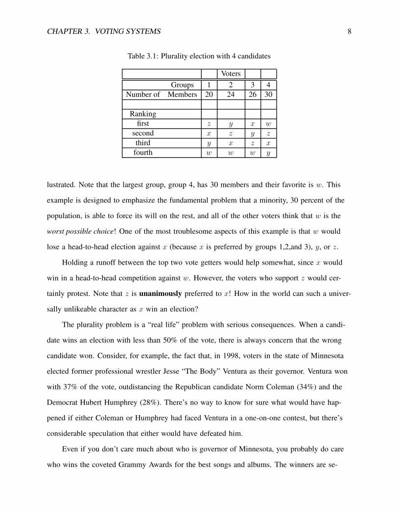
Table 3.1: Plurality election with 4 candidates
VotersGroups 1 2 3 4
Number of Members 20 24 26 30
Rankingfirst z y x w
second x z y z
third y x z x
fourth w w w y
lustrated. Note that the largest group, group 4, has 30 members and their favorite is w. This
example is designed to emphasize the fundamental problem that a minority, 30 percent of the
population, is able to force its will on the rest, and all of the other voters think that w is the
worst possible choice! One of the most troublesome aspects of this example is that w would
lose a head-to-head election against x (because x is preferred by groups 1,2,and 3), y, or z.
Holding a runoff between the top two vote getters would help somewhat, since x would
win in a head-to-head competition against w. However, the voters who support z would cer-
tainly protest. Note that z is unanimously preferred to x! How in the world can such a univer-
sally unlikeable character as x win an election?
The plurality problem is a “real life” problem with serious consequences. When a candi-
date wins an election with less than 50% of the vote, there is always concern that the wrong
candidate won. Consider, for example, the fact that, in 1998, voters in the state of Minnesota
elected former professional wrestler Jesse “The Body” Ventura as their governor. Ventura won
with 37% of the vote, outdistancing the Republican candidate Norm Coleman (34%) and the
Democrat Hubert Humphrey (28%). There’s no way to know for sure what would have hap-
pened if either Coleman or Humphrey had faced Ventura in a one-on-one contest, but there’s
considerable speculation that either would have defeated him.
Even if you don’t care much about who is governor of Minnesota, you probably do care
who wins the coveted Grammy Awards for the best songs and albums. The winners are se-
CHAPTER 3. VOTING SYSTEMS 9
lected by a plurality vote with 5 nominees on the ballot. There is often concern that the best
performers do not win. Music reporter Robert Hilburn suggested they consider changing their
voting procedure, noting, “Looking over previous Grammy contests, it’s easy to see where
strong albums may have drawn enough votes from each other to let a compromise choice win.
In 1985, two of the great albums of the decade-Bruce Springsteen’s "Born in the U.S.A." and
Prince’s "Purple Rain"-went head to head in the best album category, allowing Lionel Richie’s
far less memorable "Can’t Slow Down" to get more votes” (Hilburn, February 28, 2002). Clever
voters might try to outsmart the system, voting for their second-ranked alternative in order to
stop a weak candidate from winning. Dishonest voting is euphemistically called strategic vot-
ing in the literature.
The plurality problem has been known for centuries. It was a focus of concern in French
academic circles in the late 1700s. Two extremely interesting characters are the philosopher/scientists
Jean-Charles de Borda and the Marquis de Condorcet. Recall that it was a time of revolution,
both in America and in France. The philosophy of democracy was becoming well accepted.
The Marie Jean Antoine Nicolas Caritat, Marquis de Condorcet (1743-1794), was an extremely
influential philosopher of the Enlightenment, studying not only voting (Condorcet, 1785), but
also publishing on the rights of women, slavery and free markets. He was highly placed in
academic circles, an eager proponent of revolution against the King and, eventually, elected to
the legislature (and then later imprisoned by an opposing faction). He is credited with a com-
ment which translates as, “The apparent will of the plurality may in fact be the complete oppo-
site of their true will” (cited in Mackenzie, 2000b). Condorcet proposed a system of voting in
which alternatives were paired off for comparison. Traveling in the same circles as Condorcet
was Borda (1733-1799), an explorer, soldier, and scholar whose study of physics and mathe-
matics had wide-ranging impact on science. He agreed with Condorcet on the shortcomings of
the plurality system and he also proposed a new election procedure based on rank order vot-
ing. His manuscript, which was written sometime between 1781 and 1784 (see Saari, 1994),
indicates that he had previously presented his results on June 16, 1770 (Borda, 1781). It ap-

CHAPTER 3. VOTING SYSTEMS 10
pears that Borda had the best of it in the eyes of the French because, after the French Revo-
lution (and until Napoleon took over) the Borda procedure was used in French elections. The
Borda count fell into disuse after that, only to be revived in the modern era for rankings in
American sports. Variants are used in legislative elections in the Pacific Island countries of
Kiribati and Nauru (Reilly, 2002).
The debate between Borda and Condorcet has framed research on elections for two cen-
turies. In the next section we consider Borda’s method.
3.3 Exercises
1. Is there any way to win a majority of the vote without also winning a plurality of the
vote?
2. Suppose there are 50 shares of stock in a company and the stockholders are allowed to
vote on company policy. Each stockholder is allowed to cast one vote per share owned
in a private ballot box. No voter’s ballots has his/her name on it. Does this system vio-
late the criterion of neutrality or anonymity?
3. This example has 50 voters and 3 alternatives.
Voters
Groups 1 2 3
Number of Members 24 16 10
Ranking
first x y x
second y z z
third z x y
(a) Find the majority rule winner, if there is one.
(b) Calculate the plurality vote totals for the candidates, find the winner.
CHAPTER 3. VOTING SYSTEMS 11
(c) Does the plurality winner have a majority of the votes?
(d) Confirm that a runoff election will choose the same winner.
(e) If the winner of the each type of election is compared one-on-one against each of
the other candidates, is it a winner?
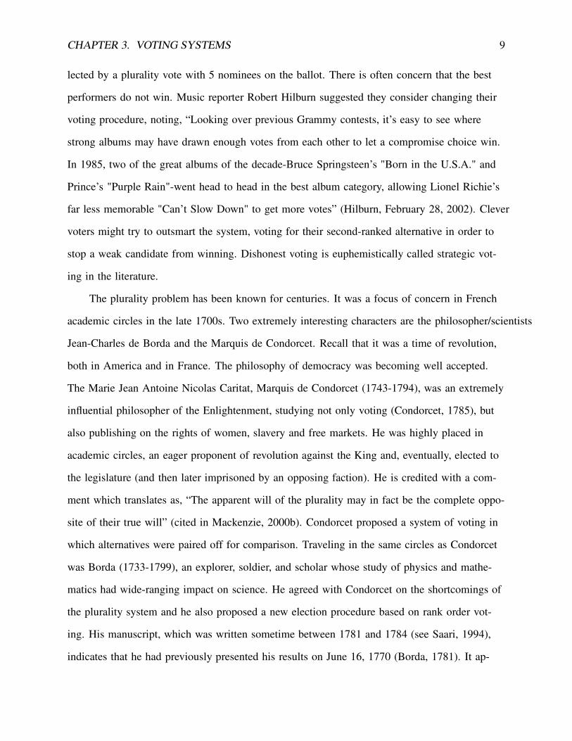
4. This example has 50 voters and 3 alternatives.
Voters
Groups 1 2 3
Number of Members 24 16 10
Ranking
first x y z
second y z y
third z x x
(a) Which candidate would win a plurality election?
(b) Does the plurality winner have a majority of the votes?
(c) If there is a runoff election between the top two vote getters, which candidate will
be the winner?
(d) If the winner of the each type of election is compared one-on-one against each of
the other candidates, is it a winner?
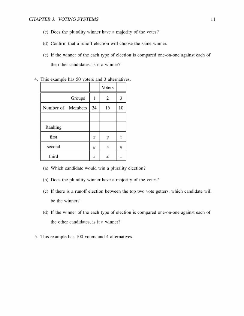
5. This example has 100 voters and 4 alternatives.
CHAPTER 3. VOTING SYSTEMS 12
Voters
Groups 1 2 3 4
Number of Members 24 19 21 36
Ranking
first x y z w
second w z x x
third z x y y
fourth y w w z
(a) Find the plurality winner.
(b) Does the plurality winner have a majority of the votes?
(c) If there is a runoff election between the top two vote getters, which candidate will
win?
(d) Suppose that, after the plurality vote, only one candidate is eliminated, and then
another three-way plurality election is held. Will any of the candidates win a ma-
jority? If not, which candidate will win a runoff election between the top two vote
getters?
6. In 2003, the voters of California were presented with an interesting choice. First, do you
want to remove Governor Gray Davis? Second, if Davis is to be replaced, which of the
following 150 candidates would you most prefer? California law states that if the num-
ber who answer yes to the first question is more than 50% of the votes cast, then the
candidate who receives the most votes will become governor. About 54% of the voters
wanted to remove Davis, and the plurality winner of the second vote was body builder &
movie star Arnold Schwartzenegger. Consider these questions about the 2003 California
election.
CHAPTER 3. VOTING SYSTEMS 13
(a) Can we be sure that a majority (or even a plurality) prefer Schwartzenegger to
Davis as governor?
(b) The results indicated that 46% of the people voted to keep Davis, but they lost.
What percentage of the vote must the replacement receive in order to take office?
Does that seem sensible?
(c) What incentives did voters have to vote strategically (untruthfully) in the first and
second parts of the ballot?
7. In the American criminal justice system, the members of a jury must agree unanimously
in order to reach a verdict. If the result is not unanimous when deliberations end, there
is a “hung jury” and a mistrial is declared. Explain why this system does not satisfy the
principle of strong monotonicity.
8. Kenneth May showed that a system based on majority rule (in which indifferent voters
abstain) is equivalent to a system in which the voters are anonymous, the alternatives are
undifferentiated, and the procedure is strongly and weakly monotonic. In May’s treat-
ment, the voters consider 2 alternatives x and y and then cast votes by selecting a value
from the set {−1, 0, 1}. A vote of 0 to indicates indifference, while 1 indicates a prefer-
ence for x and -1 indicates a preference for y.
(a) Create a mathematical definition of majority rule, assuming that the indifferent vot-
ers are ignored.
(b) Use your definition to consider the following: the winner is x and then one voter
who favored y decides she is indifferent. If you apply your procedure for majority
rule to the new voter preference data, does the result change?
(c) Suppose there is a tie and one voter changes her mind to prefer x. Apply your pro-
cedure to find out who the winner will be.
CHAPTER 3. VOTING SYSTEMS 14
(d) On the basis of your calculations in b and c of this question, do you think your def-
inition of majority rule is consistent with the Monotonicity Principle?
3.4 Rank-order voting: The Borda Count
If you are a fan of college football, you may be aware of the fact that (until 2006, at least)
there has been no national tournament to answer the question “which team is the best.” In-
stead, 100 (or so) college football teams are ranked at the end of the season, and eight of the
top teams are selected to play in 4 spotlighted games that are known as the Bowl Champi-
onship Series. The top two ranked teams play in the national championship game, and after
that game, there is another series of votes intended to rank all of the teams from top to bottom.
The formula used by the BCS to decide which teams should play in the national champi-
onship game has been a source of frustration and controversy. In 2001, the University of Ne-
braska was soundly defeated by the University of Colorado in the final regular season game.
That loss prevented Nebraska from winning the Northern division of the Big 12 conference
and it was not in the Conference championship game (which Colorado won). Nevertheless,
the BCS scores had Nebraska ahead of Colorado and the Nebraska Cornhuskers were selected
to face the University of Miami in the championship game. Nebraska was soundly defeated,
giving grounds to the contention that the BCS had chosen the wrong team. At the end of the
2003 season, the University of Southern California was not selected for the championship
game, even though the polls of writers and coaches placed USC in the top two. Decisions
like that have led to a chorus of complaints over the years, summarized aptly a student sports
writer at the University of Kansas: division 1A college football uses “what may be the most
complicated monstrosity on the planet” (Bauer, December 8, 2004, p. 2) to rank the teams.
The people who run the BCS are not oblivious to the criticism of their methods of rank-
ing teams, and every few years, they make repairs in their voting system. They raise or lower
the weight put on the votes cast by coaches, sports writers, and, strangely enough, computers!
CHAPTER 3. VOTING SYSTEMS 15
So far, at least, they have not strayed far from the same basic system. Individuals (coaches,
writers, and computers) are asked to provide rankings of the top 25 teams. The many individ-
ual rankings are summed to build an overall ranking. This is a variant of the method that was
proposed by Jean-Charles de Borda (de Borda, 1781).
3.4.1 The Borda Count
The Borda count, which we label BC, is a method of combining the rankings of many indi-
vidual voters. Suppose there are k alternatives. The voters rank the alternatives and assign in-
teger scores to them, beginning with 0 (for the worst) stepping up in integer units to k − 1 (for
the best). The rankings assigned by the voters are summed and the alternative with the largest
Borda count is the winner. The Borda count generates a complete, transitive social ordering of
the alternatives.
In mathematical terms, each voter submits a vector of scores that are keyed to the list of
candidates. If the candidates are {x, y, z} and voter i submits the Borda vector vi = (0, 2, 1),
that means that the voter thinks y is the best, z is second, and x is the worst. The Borda count
earned by a candidate j is the sum of rankings assigned by the voters,∑n
i=1vij. The notation
x �BC y to indicates that x defeats y in the Borda count. Although we do not concern our-
selves with ties in this chapter, we should mention that voters are allowed to register indiffer-
ence by assigning two alternatives the same value. For example, (0.5, 0.5, 2) indicates that x
and y are equally desirable (one vote is split between them), and both are less appealing than
z.
The Borda count works sensibly in many situations. For example, if all of the voters
agree about the ranking for all of the alternatives, it is easy to see that the Borda count gives
a meaningful reflection of their rankings. The rankings assigned by the 3 voters are presented
in the top part of Table 3.2. The Borda table, shown in the bottom half of the figure, illus-
trates the numerical vectors that represent the Borda votes. This demonstrates that the “sum
of ranks” procedure used in the BCS and other poll-style ranking systems is the same as the

CHAPTER 3. VOTING SYSTEMS 16
Table 3.2: Borda Count with Homogeneous Voters
Voter Preference Profile
Voter RankingsVoter: 1 2 3
Rankingsfirst x x x
second y y y
third z z z
Borda Count Table
Borda Votes Borda CountVoter: 1 2 3
Alternativesx 2 2 2 6y 1 1 1 3z 0 0 0 0
Borda count. It is, of course, painfully obvious that x should win. It is the most-preferred al-
ternative for all of the voters and it has the highest Borda count.
A system of this sort has been the basis of many ranking systems used in sports and en-
tertainment. Although there are bitter squabbles about the outcomes of these ranking proce-
dures, the commentary in the public media seldom considers the possibility that there is a fun-
damental problem in the basic idea of the Borda count itself. Very peculiar–even alarming–
things can happen with the Borda count.
3.4.2 A Paradox in the Borda Procedure
The problem that we now introduce has sometimes been called the “Inverted-Order Paradox”
or the “Winner Turns Loser Paradox”. It is a famous example that has been widely investi-
gated (Riker, 1982, p. 82; Fishburn, 1974). There are seven voters, {1, 2, 3, 4, 5, 6, 7} and four
alternatives, {w, x, y, z}. In Table 3.3, the columns represent the Borda voting vectors assigned
CHAPTER 3. VOTING SYSTEMS 17
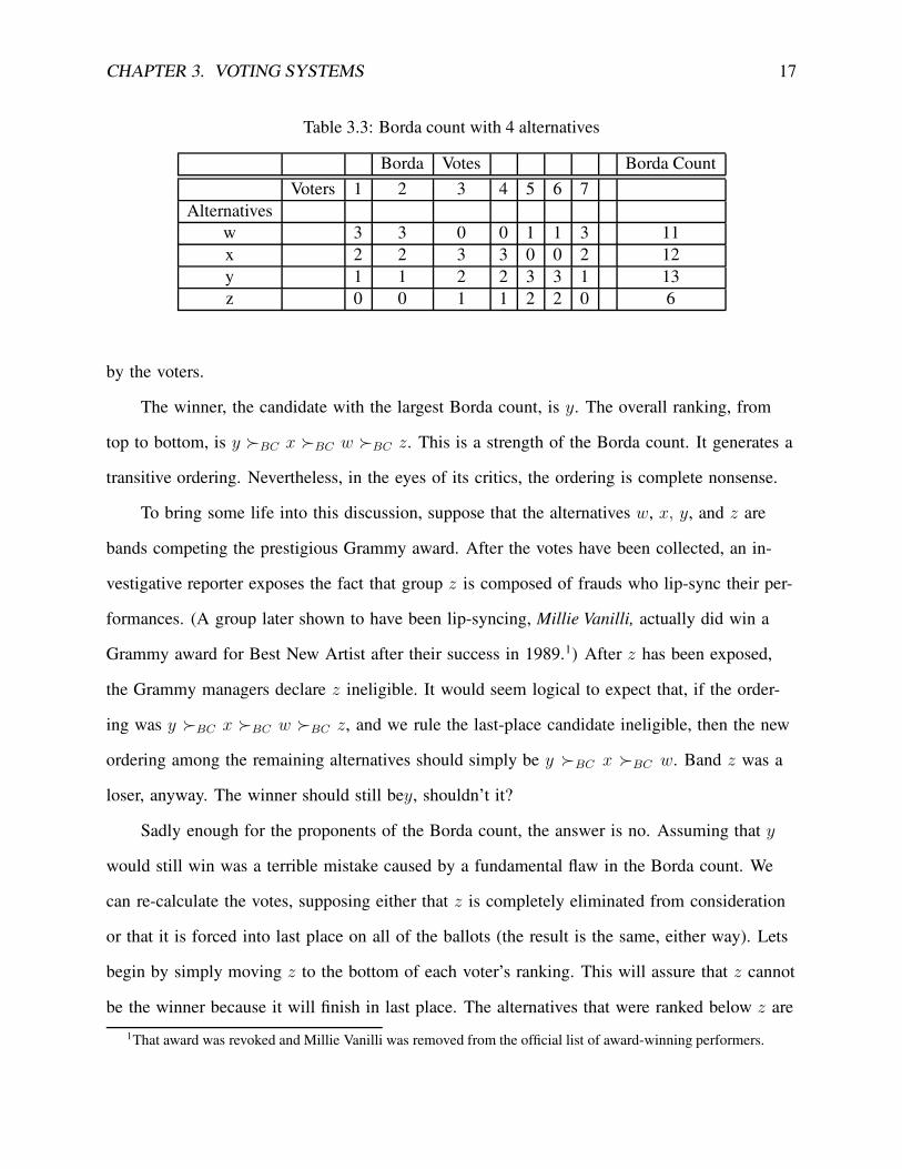
Table 3.3: Borda count with 4 alternatives
Borda Votes Borda CountVoters 1 2 3 4 5 6 7
Alternativesw 3 3 0 0 1 1 3 11x 2 2 3 3 0 0 2 12y 1 1 2 2 3 3 1 13z 0 0 1 1 2 2 0 6
by the voters.
The winner, the candidate with the largest Borda count, is y. The overall ranking, from
top to bottom, is y �BC x �BC w �BC z. This is a strength of the Borda count. It generates a
transitive ordering. Nevertheless, in the eyes of its critics, the ordering is complete nonsense.
To bring some life into this discussion, suppose that the alternatives w, x, y, and z are
bands competing the prestigious Grammy award. After the votes have been collected, an in-
vestigative reporter exposes the fact that group z is composed of frauds who lip-sync their per-
formances. (A group later shown to have been lip-syncing, Millie Vanilli, actually did win a
Grammy award for Best New Artist after their success in 1989.1) After z has been exposed,
the Grammy managers declare z ineligible. It would seem logical to expect that, if the order-
ing was y �BC x �BC w �BC z, and we rule the last-place candidate ineligible, then the new
ordering among the remaining alternatives should simply be y �BC x �BC w. Band z was a
loser, anyway. The winner should still bey, shouldn’t it?
Sadly enough for the proponents of the Borda count, the answer is no. Assuming that y
would still win was a terrible mistake caused by a fundamental flaw in the Borda count. We
can re-calculate the votes, supposing either that z is completely eliminated from consideration
or that it is forced into last place on all of the ballots (the result is the same, either way). Lets
begin by simply moving z to the bottom of each voter’s ranking. This will assure that z cannot
be the winner because it will finish in last place. The alternatives that were ranked below z are1That award was revoked and Millie Vanilli was removed from the official list of award-winning performers.
CHAPTER 3. VOTING SYSTEMS 18
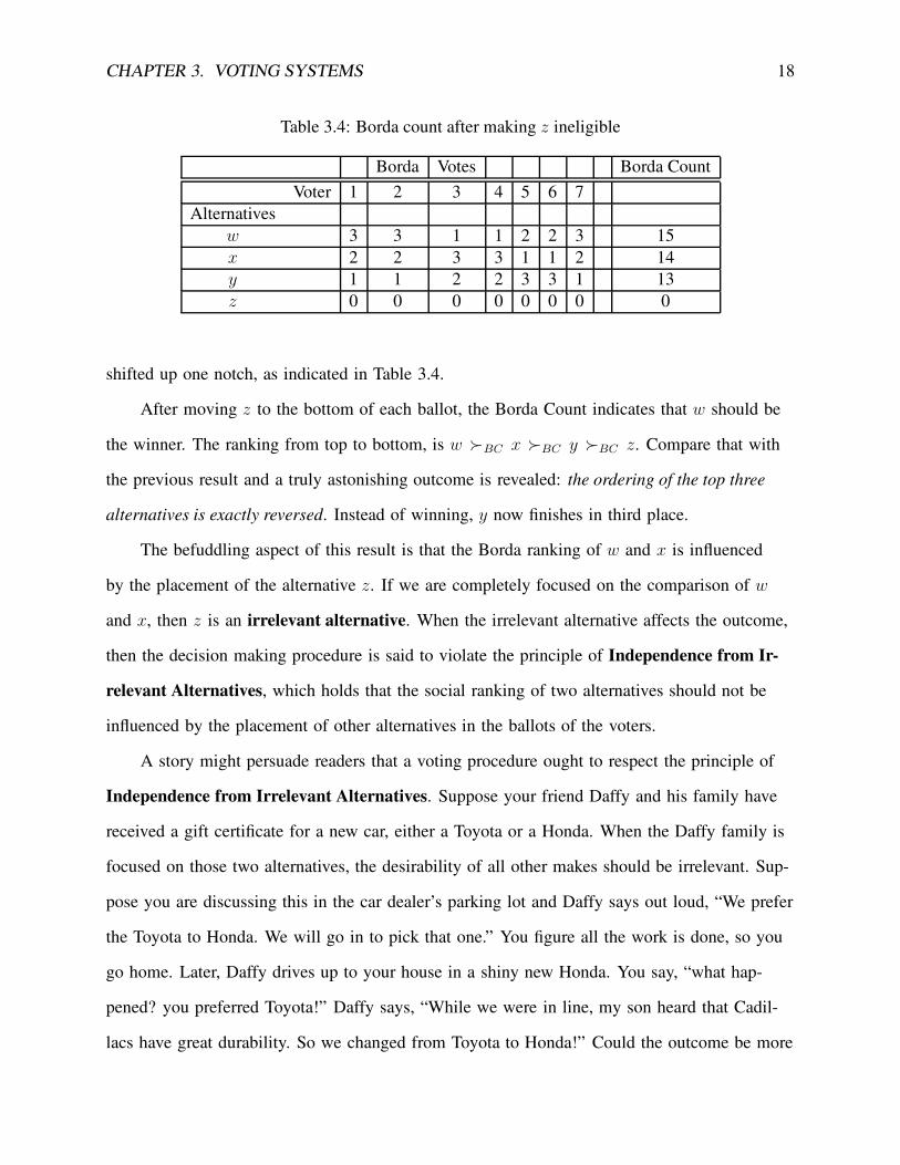
Table 3.4: Borda count after making z ineligible
Borda Votes Borda CountVoter 1 2 3 4 5 6 7
Alternativesw 3 3 1 1 2 2 3 15x 2 2 3 3 1 1 2 14y 1 1 2 2 3 3 1 13z 0 0 0 0 0 0 0 0
shifted up one notch, as indicated in Table 3.4.
After moving z to the bottom of each ballot, the Borda Count indicates that w should be
the winner. The ranking from top to bottom, is w �BC x �BC y �BC z. Compare that with
the previous result and a truly astonishing outcome is revealed: the ordering of the top three
alternatives is exactly reversed. Instead of winning, y now finishes in third place.
The befuddling aspect of this result is that the Borda ranking of w and x is influenced
by the placement of the alternative z. If we are completely focused on the comparison of w
and x, then z is an irrelevant alternative. When the irrelevant alternative affects the outcome,
then the decision making procedure is said to violate the principle of Independence from Ir-
relevant Alternatives, which holds that the social ranking of two alternatives should not be
influenced by the placement of other alternatives in the ballots of the voters.
A story might persuade readers that a voting procedure ought to respect the principle of
Independence from Irrelevant Alternatives. Suppose your friend Daffy and his family have
received a gift certificate for a new car, either a Toyota or a Honda. When the Daffy family is
focused on those two alternatives, the desirability of all other makes should be irrelevant. Sup-
pose you are discussing this in the car dealer’s parking lot and Daffy says out loud, “We prefer
the Toyota to Honda. We will go in to pick that one.” You figure all the work is done, so you
go home. Later, Daffy drives up to your house in a shiny new Honda. You say, “what hap-
pened? you preferred Toyota!” Daffy says, “While we were in line, my son heard that Cadil-
lacs have great durability. So we changed from Toyota to Honda!” Could the outcome be more
CHAPTER 3. VOTING SYSTEMS 19
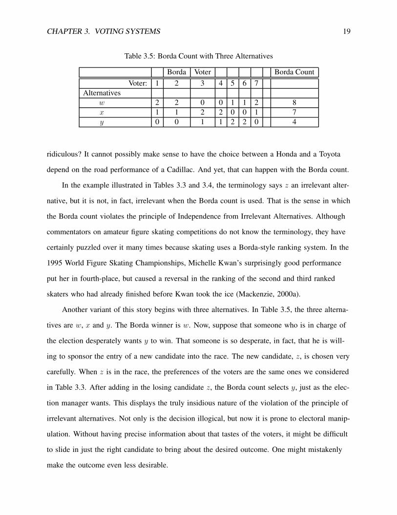
Table 3.5: Borda Count with Three Alternatives
Borda Voter Borda CountVoter: 1 2 3 4 5 6 7
Alternativesw 2 2 0 0 1 1 2 8x 1 1 2 2 0 0 1 7y 0 0 1 1 2 2 0 4
ridiculous? It cannot possibly make sense to have the choice between a Honda and a Toyota
depend on the road performance of a Cadillac. And yet, that can happen with the Borda count.
In the example illustrated in Tables 3.3 and 3.4, the terminology says z an irrelevant alter-
native, but it is not, in fact, irrelevant when the Borda count is used. That is the sense in which
the Borda count violates the principle of Independence from Irrelevant Alternatives. Although
commentators on amateur figure skating competitions do not know the terminology, they have
certainly puzzled over it many times because skating uses a Borda-style ranking system. In the
1995 World Figure Skating Championships, Michelle Kwan’s surprisingly good performance
put her in fourth-place, but caused a reversal in the ranking of the second and third ranked
skaters who had already finished before Kwan took the ice (Mackenzie, 2000a).
Another variant of this story begins with three alternatives. In Table 3.5, the three alterna-
tives are w, x and y. The Borda winner is w. Now, suppose that someone who is in charge of
the election desperately wants y to win. That someone is so desperate, in fact, that he is will-
ing to sponsor the entry of a new candidate into the race. The new candidate, z, is chosen very
carefully. When z is in the race, the preferences of the voters are the same ones we considered
in Table 3.3. After adding in the losing candidate z, the Borda count selects y, just as the elec-
tion manager wants. This displays the truly insidious nature of the violation of the principle of
irrelevant alternatives. Not only is the decision illogical, but now it is prone to electoral manip-
ulation. Without having precise information about that tastes of the voters, it might be difficult
to slide in just the right candidate to bring about the desired outcome. One might mistakenly
make the outcome even less desirable.
CHAPTER 3. VOTING SYSTEMS 20
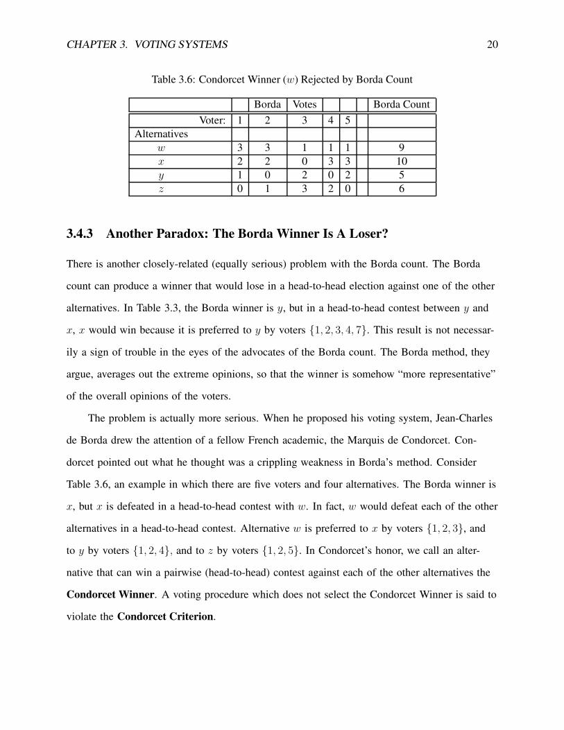
Table 3.6: Condorcet Winner (w) Rejected by Borda Count
Borda Votes Borda CountVoter: 1 2 3 4 5
Alternativesw 3 3 1 1 1 9x 2 2 0 3 3 10y 1 0 2 0 2 5z 0 1 3 2 0 6
3.4.3 Another Paradox: The Borda Winner Is A Loser?
There is another closely-related (equally serious) problem with the Borda count. The Borda
count can produce a winner that would lose in a head-to-head election against one of the other
alternatives. In Table 3.3, the Borda winner is y, but in a head-to-head contest between y and
x, x would win because it is preferred to y by voters {1, 2, 3, 4, 7}. This result is not necessar-
ily a sign of trouble in the eyes of the advocates of the Borda count. The Borda method, they
argue, averages out the extreme opinions, so that the winner is somehow “more representative”
of the overall opinions of the voters.
The problem is actually more serious. When he proposed his voting system, Jean-Charles
de Borda drew the attention of a fellow French academic, the Marquis de Condorcet. Con-
dorcet pointed out what he thought was a crippling weakness in Borda’s method. Consider
Table 3.6, an example in which there are five voters and four alternatives. The Borda winner is
x, but x is defeated in a head-to-head contest with w. In fact, w would defeat each of the other
alternatives in a head-to-head contest. Alternative w is preferred to x by voters {1, 2, 3}, and
to y by voters {1, 2, 4}, and to z by voters {1, 2, 5}. In Condorcet’s honor, we call an alter-
native that can win a pairwise (head-to-head) contest against each of the other alternatives the
Condorcet Winner. A voting procedure which does not select the Condorcet Winner is said to
violate the Condorcet Criterion.

CHAPTER 3. VOTING SYSTEMS 21
3.4.4 Inside the Guts of the Borda Count
The ranking created by the Borda count is vulnerable to manipulation by the addition or sub-
traction of candidates. By working on a few examples, one can gain some good working knowl-
edge of what kinds of changes will make a difference. One of the clearest examples is found
by comparing an election with two candidates against an election with three candidates. Sup-
pose there are 100 voters and they are divided into two groups. There are 60 voters in group 1
and they prefer x to y. Formally speaking,
Group 1 : x �i y for i ∈ {1, 2, . . . , 60}.
There are 40 voters on the other side of the issue,
Group 2 : y �i x for i ∈ {61, 62, . . .100}.
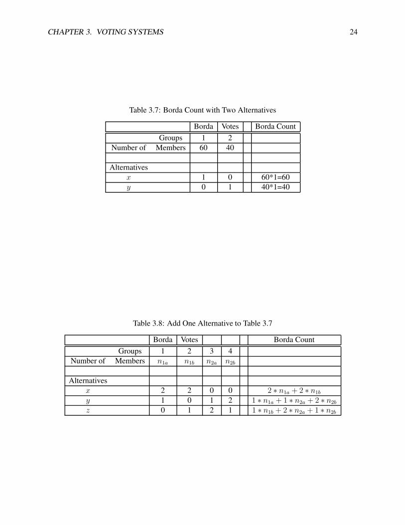
The Borda count is summarized in Table 3.7. Since group 1 has the most voters, its favorite is
the winner.
Next, suppose that a third alternative is added, and it is very similar to the loser, y. We
want to insert this new alternative into the preferences of the voters so that z is always right
next to y. Because z is always grouped together with y, it is sometimes called a clone. (One
standard for voting procedures is that their outcomes should not be changed by the addition
of redundant alternatives (clones). This example is intended to show that the Borda count is
not “cloneproof”). There are four possible orderings. The first two new orderings are found by
placing z about y in the tastes of group 1:
• Group 1a: x �i y �i z
• Group 1b: x �i z �i y
The last two are obtained by inserting z into the preferences of group 2:

CHAPTER 3. VOTING SYSTEMS 22
• Group 2a: z �i y �i x
• Group 2b: y �i z �i x
By inserting z, which is very similar to y in the eyes of the voters, we thus obtain preferences
for four groups. The relative sizes of these groups are referred to as n1a, n1b, n2a, and n2b in
Table 3.8.
Suppose that the original groups are split exactly in half, so n1a = 30, n1b = 30, n2a = 20,
and n2b = 20. With that even division within the two groups, the Borda count is 120, 90, 90
for x, y, and z, respectively. Since y is similar to z in the eyes of the voters, the result seems
plausible because y and z are tied in the Borda count. The original winner, the most favored
alternative of the majority group, still wins.
We can make some magic by fiddling with the sizes of the subgroups. Keep in mind that
there are always 60 voters for whom x is the most attractive alternative and there are always
40 for whom x is the least attractive. The only manipulation that we consider is the subdivi-
sion of the original two groups. (If you use a computer spreadsheet, it is pretty easy to con-
sider lots of conjectures.) For most of the examples that you try, the winner will be x, but
there are some exceptions. The exceptions are found when there are many voters who have y
preferred to z. That is, if you increase the values of n1a and n2b enough, then the Borda win-
ner will change from x to y. If the groups are divided n1a = 50, n1b = 10, n2a = 5, and
n2b = 35, then the Borda counts for x, y, and z are 120, 125, and 105. Even though x is still
the first-ranked alternative for 60 of 100 voters, the alternative y is the Borda winner.
The algebra of the situation is enlightening. Alternative y will defeat x (i.e., have a higher
Borda count) if
1 ∗ n1a + 1 ∗ n2a + 2 ∗ n2b > 2 ∗ n1a + 2 ∗ n1b
which is easily simplified:
n1a + 2 ∗ n1b − n2a − 2 ∗ n2b < 0
Keeping in mind that 0 ≤ n1b ≤ 60 and n1b = 60 − n1a as well as 0 ≤ n2a ≤ 40 and
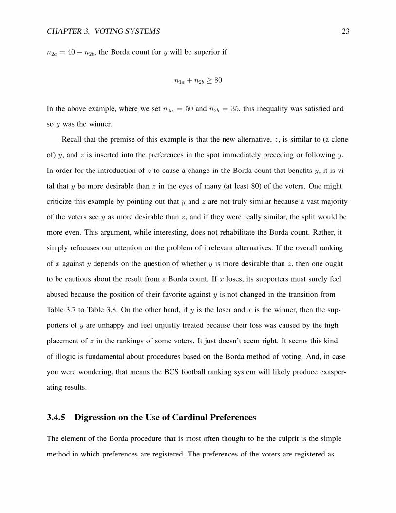
CHAPTER 3. VOTING SYSTEMS 23
n2a = 40 − n2b, the Borda count for y will be superior if
n1a + n2b ≥ 80
In the above example, where we set n1a = 50 and n2b = 35, this inequality was satisfied and
so y was the winner.
Recall that the premise of this example is that the new alternative, z, is similar to (a clone
of) y, and z is inserted into the preferences in the spot immediately preceding or following y.
In order for the introduction of z to cause a change in the Borda count that benefits y, it is vi-
tal that y be more desirable than z in the eyes of many (at least 80) of the voters. One might
criticize this example by pointing out that y and z are not truly similar because a vast majority
of the voters see y as more desirable than z, and if they were really similar, the split would be
more even. This argument, while interesting, does not rehabilitate the Borda count. Rather, it
simply refocuses our attention on the problem of irrelevant alternatives. If the overall ranking
of x against y depends on the question of whether y is more desirable than z, then one ought
to be cautious about the result from a Borda count. If x loses, its supporters must surely feel
abused because the position of their favorite against y is not changed in the transition from
Table 3.7 to Table 3.8. On the other hand, if y is the loser and x is the winner, then the sup-
porters of y are unhappy and feel unjustly treated because their loss was caused by the high
placement of z in the rankings of some voters. It just doesn’t seem right. It seems this kind
of illogic is fundamental about procedures based on the Borda method of voting. And, in case
you were wondering, that means the BCS football ranking system will likely produce exasper-
ating results.
3.4.5 Digression on the Use of Cardinal Preferences
The element of the Borda procedure that is most often thought to be the culprit is the simple
method in which preferences are registered. The preferences of the voters are registered as
CHAPTER 3. VOTING SYSTEMS 24
Table 3.7: Borda Count with Two Alternatives
Borda Votes Borda CountGroups 1 2
Number of Members 60 40
Alternativesx 1 0 60*1=60y 0 1 40*1=40
Table 3.8: Add One Alternative to Table 3.7
Borda Votes Borda CountGroups 1 2 3 4
Number of Members n1a n1b n2a n2b
Alternativesx 2 2 0 0 2 ∗ n1a + 2 ∗ n1b
y 1 0 1 2 1 ∗ n1a + 1 ∗ n2a + 2 ∗ n2b
z 0 1 2 1 1 ∗ n1b + 2 ∗ n2a + 1 ∗ n2b
CHAPTER 3. VOTING SYSTEMS 25
integer-valued rankings. If a voter thinks that x is much better (or just a little better) than y,
and y is much (or just a little bit better) than z, the ranking will be submitted as 1-2-3 and the
magnitude of preference is ignored. A proponent of cardinal preferences would rather have us
figure out a way to precisely measure these differences so that the voter could submit a vote
like 1-1.8-2.0 to signify the fact that the first one is the best and the other two are far worse.
In the advanced literature on social choice theory, there are in fact some highly prestigious au-
thors, such as Nobel Prize Winners John Nash (1950) and John Harsanyi (1955) who have ad-
vocated decision-making based on these fine-grained evaluations. John Nash, the game theorist
whose life story was the basis of the movie A Beautiful Mind, was probably the first to contend
that these cardinal scores should be collected and multiplied together to create a social ranking.
In his honor, Riker calls this the Nash method (see Riker, 1982).
The use of cardinal scores has intuitive appeal. Harsanyi offers a rigorous mathematical
argument in favor of this system, contending that it optimizes the welfare of the community in
a utilitarian sense. That may be, but, as Riker demonstrates (1982, p. 110-111), the problem
of irrelevant alternatives remains. In fact, the problem may be more severe in the Nash method
than in the Borda method. In the Borda method, the fact that voters are restricted to casting
votes in integer values limits the extent to which the placement of z might influence the com-
parison of x and y. In a cardinal election, the votes can range across a continuum, seemingly
opening up a much larger range of outcomes that are influenced by irrelevant alternatives.
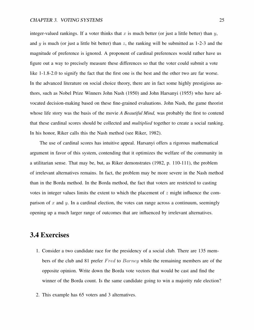
3.4 Exercises
1. Consider a two candidate race for the presidency of a social club. There are 135 mem-
bers of the club and 81 prefer Fred to Barney while the remaining members are of the
opposite opinion. Write down the Borda vote vectors that would be cast and find the
winner of the Borda count. Is the same candidate going to win a majority rule election?
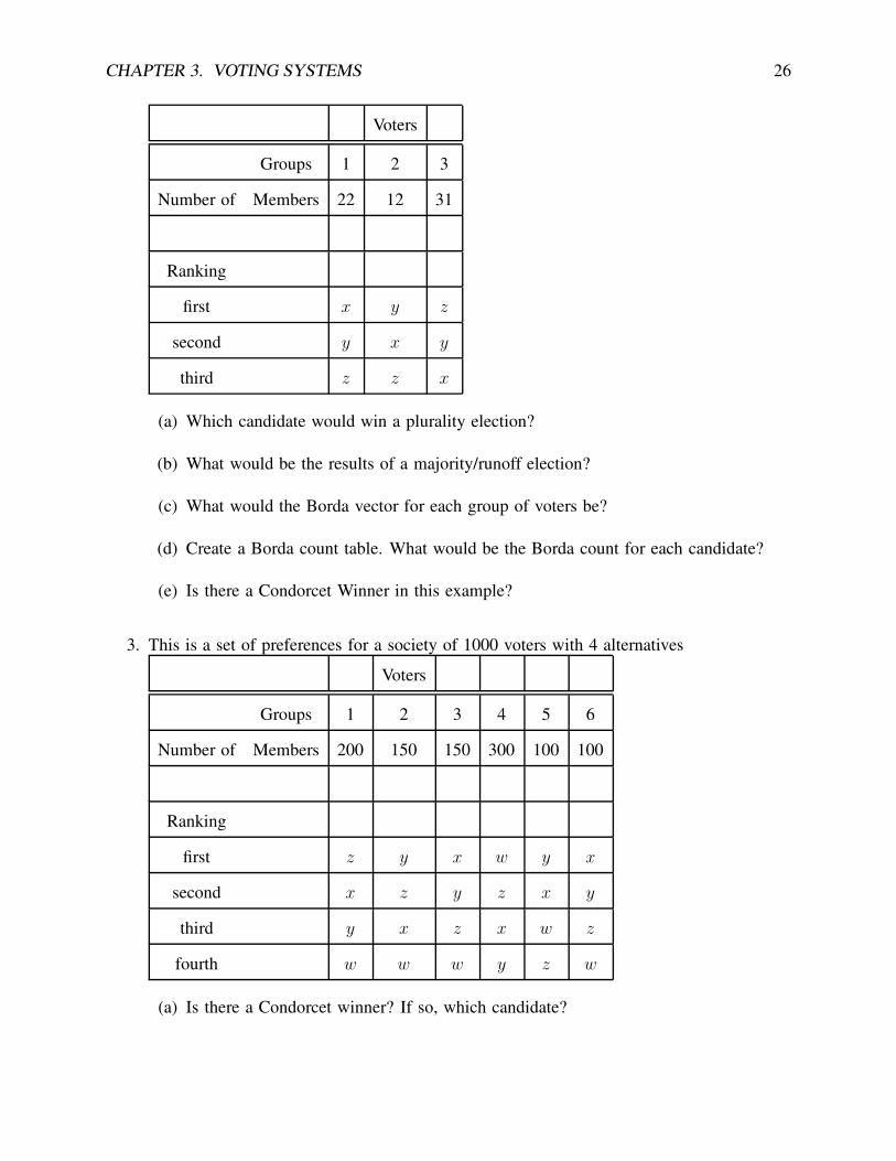
2. This example has 65 voters and 3 alternatives.
CHAPTER 3. VOTING SYSTEMS 26
Voters
Groups 1 2 3
Number of Members 22 12 31
Ranking
first x y z
second y x y
third z z x
(a) Which candidate would win a plurality election?
(b) What would be the results of a majority/runoff election?
(c) What would the Borda vector for each group of voters be?
(d) Create a Borda count table. What would be the Borda count for each candidate?
(e) Is there a Condorcet Winner in this example?
3. This is a set of preferences for a society of 1000 voters with 4 alternatives
Voters
Groups 1 2 3 4 5 6
Number of Members 200 150 150 300 100 100
Ranking
first z y x w y x
second x z y z x y
third y x z x w z
fourth w w w y z w
(a) Is there a Condorcet winner? If so, which candidate?
CHAPTER 3. VOTING SYSTEMS 27
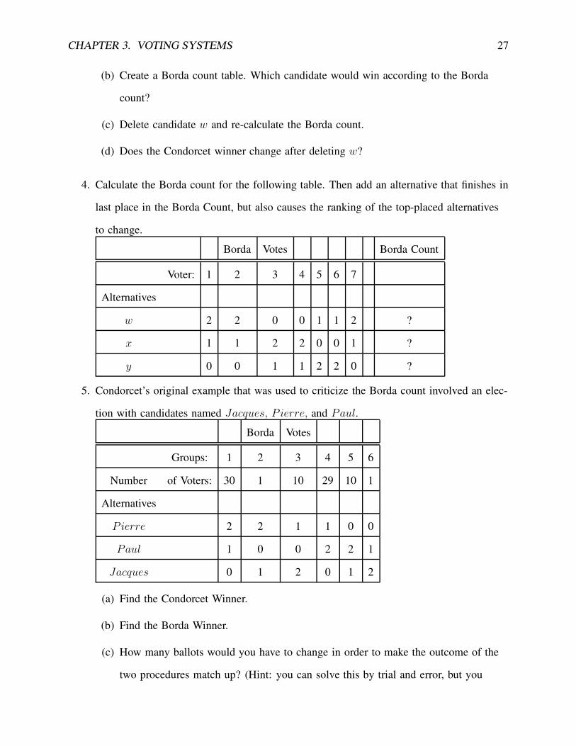
(b) Create a Borda count table. Which candidate would win according to the Borda
count?
(c) Delete candidate w and re-calculate the Borda count.
(d) Does the Condorcet winner change after deleting w?
4. Calculate the Borda count for the following table. Then add an alternative that finishes in
last place in the Borda Count, but also causes the ranking of the top-placed alternatives
to change.
Borda Votes Borda Count
Voter: 1 2 3 4 5 6 7
Alternatives
w 2 2 0 0 1 1 2 ?
x 1 1 2 2 0 0 1 ?
y 0 0 1 1 2 2 0 ?
5. Condorcet’s original example that was used to criticize the Borda count involved an elec-
tion with candidates named Jacques, P ierre, and Paul.Borda Votes
Groups: 1 2 3 4 5 6
Number of Voters: 30 1 10 29 10 1
Alternatives
Pierre 2 2 1 1 0 0
Paul 1 0 0 2 2 1
Jacques 0 1 2 0 1 2
(a) Find the Condorcet Winner.
(b) Find the Borda Winner.
(c) How many ballots would you have to change in order to make the outcome of the
two procedures match up? (Hint: you can solve this by trial and error, but you
CHAPTER 3. VOTING SYSTEMS 28
should not have to. Recall that the Borda count equals the aggregated pairwise
vote.)
3.5 Sequential Pairwise Comparisons
The critics of the Bowl Championship Series often contend that college football should adopt
a tournament format to select a national champion. A tournament is used in many other col-
lege sports as well as professional baseball, basketball and football. Would a tournament solve
the controversy over “who’s number one?” There are good reasons to be skeptical. A tourna-
ment might increase advertising revenue, but we doubt it would put an end to questions about
whether the best team was actually ranked number one at the end.
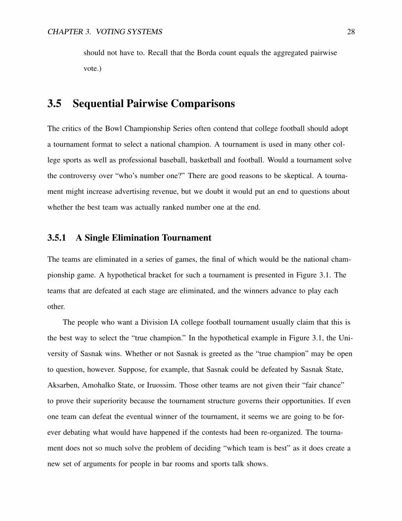
3.5.1 A Single Elimination Tournament
The teams are eliminated in a series of games, the final of which would be the national cham-
pionship game. A hypothetical bracket for such a tournament is presented in Figure 3.1. The
teams that are defeated at each stage are eliminated, and the winners advance to play each
other.
The people who want a Division IA college football tournament usually claim that this is
the best way to select the “true champion.” In the hypothetical example in Figure 3.1, the Uni-
versity of Sasnak wins. Whether or not Sasnak is greeted as the “true champion” may be open
to question, however. Suppose, for example, that Sasnak could be defeated by Sasnak State,
Aksarben, Amohalko State, or Iruossim. Those other teams are not given their “fair chance”
to prove their superiority because the tournament structure governs their opportunities. If even
one team can defeat the eventual winner of the tournament, it seems we are going to be for-
ever debating what would have happened if the contests had been re-organized. The tourna-
ment does not so much solve the problem of deciding “which team is best” as it does create a
new set of arguments for people in bar rooms and sports talk shows.
CHAPTER 3. VOTING SYSTEMS 29
Figure 3.1: Hypothetical Football Tournament
Sasnak State U.
U. of Odaroloc
U of Aksarben
U. of Amohalko
U. of Iruossim
U. of SasnakU. of Sasnak
U. of Sasnak
U. of Sasnak
Awoi State U.Awoi State U.
U. of Odaroloc
Amohalko St. U.
U. of Odaroloc
Amohalko State U.
The tournament concept, it turns out, is widely ussed, not just for sporting events, but for
political decision making as well. For example, in American elections, the candidates of the
top two political parties face each other in the general election (the “championship game”).
Those candidates are the winners of earlier contests. Like the winners of sporting tournaments,
these winners are no less open to after-the-fact challenges from contenders who did not get
their fair chance.
There is one case in which a tournament structure produces an unequivocal, certain win-
ner. If there is a Condorcet winner, one candidate (or team) that defeats each of the others in a
one-on-one competition, then that winner will be the only survivor of the tournament.
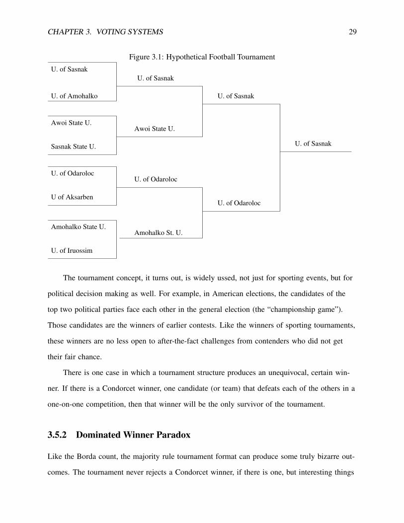
3.5.2 Dominated Winner Paradox
Like the Borda count, the majority rule tournament format can produce some truly bizarre out-
comes. The tournament never rejects a Condorcet winner, if there is one, but interesting things
CHAPTER 3. VOTING SYSTEMS 30
Table 3.9: Dominated Winner Paradox
Voter PreferencesRankings Voters: 1 2 3
first w y x
second x w z
third z x y
fourth y z w
Sequence of Votes w �M x y �M w z �M y
Figure 3.2: Tournament Structure for the Dominated Winner Paradox
w
x
w
y
y
z
z
can still happen. Perhaps the most well known is the “dominated winner paradox.” It is pos-
sible that the winner of a tournament can be unanimously defeated by another alternative. We
mean to say not just that the tournament picks the second-best or third-best, but rather, that the
tournament winner is unanimously considered inferior. The preferences in Table 3.9 are used
to illustrate this paradox. There three voters and four alternatives, w,x,y, and z. In the tour-
nament structure that is drawn in Figure 3.2, there is a a sequence of three votes. First, alter-
native x is defeated by w. Then, in the second stage, the winner, w is defeated by y, and then
the final vote pitsy against z. Note that the first outcome to be eliminated, x, is preferred to w
by every single voter. 2
2This is called the “dominated winner paradox” because, in the field of cooperative game theory, one alternativeis said to dominate another if every participant prefers it to the other.
CHAPTER 3. VOTING SYSTEMS 31
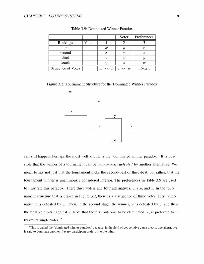
Table 3.10: Preferences for Three CandidatesVoter Groups
Rankings 1 2 3
first Thing 1 Cat in the Hat Thing 2second Thing 2 Thing 1 Cat in the Hatthird Cat in the Hat Thing 2 Thing 1
3.5.3 The Intransitivity of Majority Rule
In the first section of this chapter, we drew the reader’s attention to the concept of transitiv-
ity. Now that concept comes to the forefront again. There are majority rule examples in which
x �M y, and y �M z, but (and here’s nontransitive part) z �M x. Social comparisons some-
times lack the fundamental properties of reason and logic summarized by the principle of tran-
sitivity that is present in the tastes of voters.
Consider an example with three candidates (two Democrats, one Republican) and three
groups of voters. The Democrats, named Thing 1 and Thing 2, are pitted in a tightly contested
electoral campaign, and the winner will face the Republican candidate, named Cat in the Hat.
Lets suppose there are three equally sized groups of voters. The transitive orderings of the vot-
ers are presented in Table 3.10. Readers will note that this kind of table is slightly different
than the one used for the Borda count, but the information that it contains is the same.
It is especially important to note that the preferences of the voters are transitive. Con-
sider the preferences in Table 3.10. For Group 1 we are told that Thing 1 is preferred to Thing
2, and Thing 2 is preferred to Cat in the Hat. Then transitivity of preference implies we are
safe in concluding that Thing 1 is preferred to the Cat in the Hat by members of Group 1.
The tournament begins with Thing 1 and Thing 2 facing each other and all three groups
of voters are allowed to have their say. Since Thing 1 is preferred to Thing 2 by groups 1 and
2, Thing 1 is the winner of that stage. The final stage pits Thing 1 against Cat in the Hat, and
with the backing of groups 2 and 3, Cat in the Hat wins.
If majority rule were transitive, then we could conclude that Cat in the Hat is socially pre-
CHAPTER 3. VOTING SYSTEMS 32
ferred to Thing 2. It is a startling and truly paradoxical fact that majority rule does not support
that prediction. Majority rule does not obey the property of transitivity.
Imagine what would happen if, in the time-honored tradition of politicians, Thing 2 hires
a large team of lawyers who appeal the case to the highest court. The court might order an-
other election pitting Thing 2 against Cat in the Hat. The Cat in the Hat should do everything
he can to avoid another vote. Note that groups 1 and 3 prefer Thing 2 to Cat in the Hat, so
Thing 2 would win that final electoral competition.
Even though the individual voter preferences are transitive, the majority rule ordering is
not! This peculiar finding, sometimes called The Voter’s Paradox, means that where we ex-
pect to find logic and reason: x �M y,y �M z, and x �M z, instead we find nonsense and
irrationality: x �M y,y �M z, and z �M x. We could keep voting forever, with each win-
ner being defeated in turn. This is called a voting cycle. A person who is intransitive lacks the
fundamental properties of reason and logic and would be incapable of making decisions and
managing personal affairs. Should a society that is intransitive be viewed in the same harsh
light? For centuries, political scientists have been locked in debate over the issue.
Despite these problems, majority rule is very widely used in legislatures. There are some
arguments that can be advanced in favor of the majority rule method and to justify its con-
tinued use. By far the most important justification for the use of majority rule is offered by
May’s theorem, which we have already discussed.
The second reason why majority rule is still widely used, even though cycles are possible,
is that cycles are thought to be rare. If there are only three voters with three alternatives, and
we ignore the possibility that voters may be indifferent, then we can make a list of all possible
“societies.” There are 216 possible 3 voter societies, and a cycle can arise in 12, or approx-
imately 5.6% (Johnson, 1998, p. 23). Many computer simulation studies have been done to
try to find out how likely a cycle is to arise when the numbers of voters and alternatives are
increased. A review of several studies led Riker (1982) to contend that the probability of cy-
cles rises dramatically (near 1.0) as the number of alternatives and voters increase, while Jones
CHAPTER 3. VOTING SYSTEMS 33
et al. (1995) contended that if voter indifference is taken into account, then the probability of
cycles is not quite so high.
If cycles are possible in the real world, why don’t we observe them more often? Quite
simply, we do not use voting procedures that are designed to discover them. Election pro-
cedures are generally written so that candidates are eliminated and are not given a second
chance. Voting in legislatures is tightly controlled by party leaders who refuse to let the mem-
bers propose frivolous alternatives in a “fishing expedition”. In his discussion of the American
Constitutional Convention of 1787, Riker tells the story of a cycle that was revealed when the
delegates were attempting to formalize the system for presidential elections (1986, p. 46-7).
The cycle caused confusion and uncertainty, and eventually the matter was delegated it to a
subcommittee that was trusted to write up something good. That’s how the Electoral College
was created.
3.5 Exercises
1. The candidates in an electoral tournament are Hamilton,Joe, Frank, and Reynolds. In
the first stage, Reynolds will be paired off against Frank and Joe will face off against
Hamilton. The winners of those two contests will compete to decide the overall winner.
Draw a figure that represents this tournament.
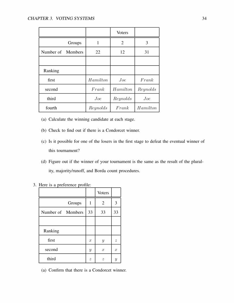
2. Here is a preference profile for the voters who are polled in the tournament described in
the previous question.
CHAPTER 3. VOTING SYSTEMS 34
Voters
Groups 1 2 3
Number of Members 22 12 31
Ranking
first Hamilton Joe Frank
second Frank Hamilton Reynolds
third Joe Reynolds Joe
fourth Reynolds Frank Hamilton
(a) Calculate the winning candidate at each stage.
(b) Check to find out if there is a Condorcet winner.
(c) Is it possible for one of the losers in the first stage to defeat the eventual winner of
this tournament?
(d) Figure out if the winner of your tournament is the same as the result of the plural-
ity, majority/runoff, and Borda count procedures.
3. Here is a preference profile:
Voters
Groups 1 2 3
Number of Members 33 33 33
Ranking
first x y z
second y x x
third z z y
(a) Confirm that there is a Condorcet winner.

CHAPTER 3. VOTING SYSTEMS 35
(b) Suppose there is a tournament in which x and y face off against each other, and
then z challenges the winner. Does the Condorcet winner also win the tournament?
(c) Can you think of any way in which to design the tournament so that the Condorcet
winner does not win the final contest of the tournament?
4. Consider the following preferences.
Voters
Groups 1 2 3
Number of Members 18 16 21
Ranking
first x y z
second y x y
third z z x
(a) Design a single elimination tournament and find the winner.
(b) Is there any way to re-design your tournament so that a different alternative will
win?
5. In the following table, we provide preferences for 7 out of 11 voters.
Voters
Groups 1 2 3 4 5 6
Number of Members 3 3 2 1 1 1
Ranking
first z y x
second x z w
third y w z
fourth w x y
CHAPTER 3. VOTING SYSTEMS 36
(a) Fill in the preferences for the last 3 columns in such a way that there is a pairwise
voting cycle in which x �P y, y �P z, and z �P x. You can insert any transitive
rankings for groups 4, 5, and 6.
(b) Choose your favorite letter from the set {x, y, z}. Design a single-elimination tour-
nament in which your selected alternative wins.
3.6 Condorcet Methods: The Round Robin Tournament
On the basis of the preceding analysis, the reader should believe that the following claims are
correct.
1. If there is a Condorcet Winner, then a single-elimination tournament format will select
that alternative.
2. If there is no Condorcet Winner, the tournament winner is determined by the pairings of
the alternatives.
The presiding officer of a town council might exercise the power to set the agenda to advan-
tage some community groups over others. There’s a charming essay about an economist and a
lawyer who studied social choice theory and then used it to hornswaggle the voters in a club
that purchased airplanes for recreational use (Riker, 1986).
To address this problem, Condorcet’s approach was to search for a method of voting that
will give a meaningful result when all of the pairwise comparisons are considered. Condorcet’s
suggested that we collect enough information from voters so that we can hold (what is now
called) a “round robin” tournament. In a round robin, each alternative faces each of the others
in a head-to-head competition.
The Condorcet Criterion states that if there is a Condorcet winner–one alternative can
defeat each of the others head-on–then it should win. If there is no Condorcet winner, then

CHAPTER 3. VOTING SYSTEMS 37
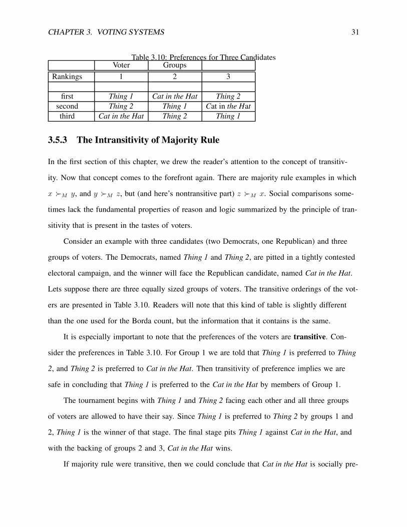
Figure 3.3: The Smith Set(a) The Smith Set is a “top cycle” (b) The Smith Set includes all alternatives
u v
w
x
y
z
u v
w
x
y
z
problem is to find a way to summarize the pairwise information and choose or shape the re-
sults into a ranking. Duncan Black, a pioneer of modern social choice research, suggested
“The reasons may not seem so overwhelmingly convincing, but we are moving in a region
where all considerations are tenuous and fine-spun; and the claims of the Condorcet criterion
to rightness seem to us much stronger than those of any other”(Black, 1958). In the time since
Condorcet, many different schemes have been proposed to summarize the outcomes of pair-
wise comparisons. Black suggested the use of a Borda Count. We consider just a few of the
many interesting proposals.
3.6.1 Searching for an Unbeatable Set of Alternatives
Here’s an obvious starting point: eliminate undesirable alternatives from consideration. Sup-
pose the alternatives under consideration are {u, v, w, x, y, z}. In Figure 3.3, the relationships
among the alternatives are represented by arrows. In this type of graph, an arrow from x to
y means that x defeats y is a pairwise competition. In panel (a) of Figure 3.3, note that u, y,
and x, the ones that are inside the dotted line, have a special quality. Each of them can de-
feat each of the others that are outside the dotted line in a head-to-head race. It seems clear
that the winner must not be drawn from {v, w, z}. Each of these can be defeated by each of
the proposals in {u, x, y}. The Smith Criterion is based on the idea that, if we can spot some
CHAPTER 3. VOTING SYSTEMS 38
“rejects” in this way, then we ought to make sure they don’t win.
Formally, the Smith set is defined as the smaller of two sets:
1. The set of all alternatives, X .
2. A subset A ⊂ X such that each member of A can defeat every member of X that is
not in A, which we call B=X − A. Formally, the Smith Criterion states if x ∈ A and y ∈ B =
X − A, x �P y.
Note we are using the plurality rule notation here, x �P y (see 3.6). Indifferent voters are
ignored. As we have seen in Figure 3.3a, the Smith set may include a voting cycle, and that’s
why some authors refer to it as the “top cycle set.” The top cycle includes only the “best of
the best.” The rest of the alternatives should be rejected.
One major shortcoming of the Smith Criterion is illustrated in Figure 3.3b. We have turned
around a few arrows, so there is no subset of alternatives in which each can defeat the rest. In
such a case, the Smith set includes all alternatives. As a result, the Smith Criterion sheds no
light at all on the problem. While the Smith criterion can be useful in ruling out alternatives in
some examples, but not too many.
3.6.2 The Win-Loss Record
A second simple approach is to choose a winner on the basis of the win-loss records. This
is often called the Copeland rule. We simply subtract the number of losses from the number
of wins for each alternative and then rank the alternatives accordingly. If one reads the sports
page during professional baseball or football seasons, the win-loss record is a very familiar
concept. While simple in principle, this procedure has many shortcomings. Most importantly,
if there is a voting cycle, then there are likely to be many ties in the win-loss column. Each
alternative will have one win and one loss in the pairwise comparisons, so none can be distin-
guished from the others. Another problem with this approach its sensitivity to the introduction
of clones. One could pad the number of wins for an alternative by making copies of the alter-
natives that it can defeat. (For Three Stooges fans, if Curly is a loser, then nominate Moe and

CHAPTER 3. VOTING SYSTEMS 39
Larry as well so that the alternatives that defeat Curly also defeat Moe and Larry.)
3.6.3 Aggregated Pairwise Voting: The Borda Count Strikes Back!
The aggregated pairwise vote is a method of evaluating a tournament. The alternatives accu-
mulate votes in their head-to-head contests and the one with the most votes wins. It creates a
transitive overall ranking, even if there is a pairwise majority rule cycle.
Suppose the voters are N = {1, 2, . . . , n} and that none of them are indifferent between
any of the alternatives. Recall that the number of voters who prefer x to y can be represented
as |{i ∈ N : x �i y}|. The aggregated vote for alternative x is the sum of the support it
receives against y and z in pairwise contests:
|{i ∈ N : x �i y}| + |{i ∈ N : x �i z}|.
The aggregated pairwise vote has a number of interesting properties. Readers should easily
convince themselves that the following claims are true:
1. A Condorcet winner (one who is undefeated by each of the others) is never ranked last
by the aggregated pairwise vote, and
2. A Condorcet loser (one that is unable to defeat any of the others) is never ranked first by
the aggregated pairwise vote.
The aggregated pairwise vote is never afflicted by the “dominated winner paradox” that was
discussed above. While the Condorcet winner does not always come out on top in an aggre-
gated pairwise vote, that candidate does not suffer the indignity of a last place finish either.
It turns out that these two properties of the aggregated pairwise vote have a powerful im-
plication: only a restricted number of paradoxical voting outcomes is possible. With two alter-
natives, the aggregated pairwise system is really just plurality rule, so we might write either
x �AP y or x �P y. If the pairwise result is x �AP y, then a supporter of Condorcet’s
CHAPTER 3. VOTING SYSTEMS 40
view of the problem would expect that the social ranking should be x �AP y �AP z or
z �AP x �AP y. As long as the procedure applied to all 3 alternatives has x preferred to y,
then everything makes sense. On the other hand, there is trouble if we observe social rankings
like y �AP x �AP z or z �AP y �AP x.
Mathematician Donald Saari offers a way to catalogue these so-called anomalies. For
a given set of voters (a preference profile), any voting procedure can be applied to rank the
pairs, {x, y}, {y, z}, {x, z}, and also give an ordering of all three alternatives, {x, y, z}. Since
the pairwise comparison is really just a plurality vote, let’s use P as the subscript for pairwise
comparisons, and we will use AP for the comparisons that take into account 3 or more alter-
natives. Saari uses the term word to refer to a combined set of pairwise and aggregated pair-
wise rankings, such as
word 1. x �P y, y �P z, x �P z, x �AP y �AP z
or
word 2. x �P y, y �P z, x �P z , z �AP y �AP x
There are 351 words possible with 3 alternatives (hint: 3 · 3 · 3 · 13 = 351). In word 1,
there is no anomaly because each of the pairwise plurality decisions is the same as the order-
ing implied by the aggregated pairwise votes. On the other hand, word 2 is very anomalous.
The pairwise comparisons are at odds with the overall ranking. In fact, recalling the first claim
above, readers should notice that word 2 is impossible. The aggregated pairwise vote could not
assign last place to the Condorcet winner, x.
Saari observes that only 135 out of the 351 words are actually possible with the aggre-
gated pairwise vote applied to three alternatives (1994, p. 186). The driving force behind that
result is the fact that the Condorcet winner can’t finish last in the aggregated pairwise vote.
The complete explanation of this result is given in the focus box on page 42.
CHAPTER 3. VOTING SYSTEMS 41
In case you were wondering why the subtitle of this section is “the Borda count strikes
back!” we are ready to give the answer: The aggregated pairwise voting procedure is equiva-
lent to the Borda count (Saari, 1994). The strengths of the aggregated pairwise vote are thus
inherited by the Borda count. Saari advocates the use of the Borda count for a number of rea-
sons, but the fact that it “is the ’natural’ extension of the standard vote between two candi-
dates” (Saari, 1994, p. 178) to an election with more candidates is one of the most persuasive
reasons.
How do we know that the two procedures equivalent? Consider a voter i for whom x �i
y �i z. The aggregation shows that i casts 2 votes for x (i prefers x to both y and z). Simi-
larly, i votes for y against z, and the aggregation records 1 vote for y. This is, of course, ex-
actly the same as casting a Borda ballot vector (2, 1, 0). The conclusion is that the Borda count
has the same information that is collected by the aggregation of pairwise votes.
The fundamental difference between plurality/majority voting and the Borda count is laid
bare by this discovery. Recall the definition of plurality rule, which is the same as majority
rule if none of the voters are indifferent.
P lurality rule : x �P y if and only if |{i ∈ N : x �i y}| > |{i ∈ N : y �i x}|
(3.6)
Note that the first terms on each side of the following inequality are the same:
Borda rule : x �BC y if and only if
|{i ∈ N : x �i y}|+ |{i ∈ N : x �i z}| > |{i ∈ N : y �i x}|+ |{i ∈ N : y �i z}|
(3.7)

CHAPTER 3. VOTING SYSTEMS 42
The Borda comparison between x and y always includes some information about the irrele-
vant alternative z. The violation of the independence from irrelevant alternatives that we en-
counter in examples involving the Borda count appears to be inherent within it. At the same
time, however, the Borda count avoids both intransitivities and the danger of allowing a Con-
dorcet loser to win an election.
===========================================
Feature Box: The Aggregated Pairwise Vote and the Borda Count.
In The Geometry of Voting, mathematics professor Donald Saari argues that the Borda
count is less prone to peculiarities than other voting methods that are based on ranked lists.
The Borda count admits only 135 out of 351 possible words (combinations of pairwise and
listwise outcomes). In contrast, other methods of tabulation allow anything (literally!) to hap-
pen. A central part of his argument is the fact that the Borda count is equivalent to aggregated
pairwise voting, and in the latter we have observed that a Condorcet winner never places last.
To see why only 135 of the possible words can occur, begin by considering all of the
Borda orderings with 3 alternatives. They are divided into three columns, representing social
orderings in which the number of ties is zero, one, or two.
1. x �BC y �BC z 7. x �BC y ≈BC z 13.x ≈BC y ≈BC z
2. x �BC z �BC y 8. x ≈BC y �BC z
3. y �BC x �BC z 9. y ≈BC z �BC x
4. y �BC z �BC x 10. y �BC z ≈BC x
5. z �BC x �BC y 11. z �BC x ≈ BCy
6. z �BC y �BC x 12. z ≈BC x �BC y
We now have to figure out which pairwise outcomes are consistent with each of these
Borda outcomes. The problem is attacked by the timeless method of “divide and conquer.”
Consider outcomes 1-6, the ones in which there are no ties. Keeping in mind the fact that
a Condorcet winner cannot finish in last place in the Borda count (and the Condorcet loser
cannot finish first), we can figure out which pairwise comparisons are possible. We focus on

CHAPTER 3. VOTING SYSTEMS 43
this one case x �BC y �BC z (and will generalize to the others).
Possible if x �BC y �BC z Not possible if x �BC y �BC z
x �P y, y �P z, x �P z x ≈P y, y �P z, x �P z x ≈P y, y �P z, x ≈P z
x �P y, y �P z, z �P x x ≈P y, y ≈P z, x �P z x ≈P y, y �P z, z �P x
x �P y, y �P z, z ≈P x x ≈P y, z �P y, x �P z x ≈P y, y ≈P z, z �P x
x �P y, z �P y, z ≈P x y �P x, y �P z, x �P z x ≈P y, y ≈P z, z ≈P x
x �P y, y ≈P z, z �P x y �P x, y ≈P z, x �P z x ≈P y, z �P y, z �P x
x �P y, y ≈P z, z �P x y �P x, z �P y, x �P z x ≈P y, z �P y, z ≈P x
x �P y, y ≈P z, z ≈P x y �P x, z �P y, z �P x y �P x, y �P z, z �P x
x �P y, z �P y, x �P z y �P x, z �P y, z ≈P x y �P x, z �P y, z �P x
x �P y, z �P y, z �P x y �P x, z ≈P y, z �P x
y �P x, y �P z, x ≈P z
There are 17 sets of pairwise contests that are consistent with x �BC y �BC z. Since the
setup of the problem is completely symmetric, the same must be true of Borda orderings 2-6.
Since 6*17=102, we have found 102 of the 135 legal words.
Next consider the six Borda outcomes that have only one tie, which are items 7-12. There
are 30 sets of pairwise outcomes that are consistent with these Borda results (five for each
one). Considering Borda ordering 7, we find that the following are the legal words.
1. x �P y, x �P z, y ≈M z, x �BC y ≈BC z
2. x �P y, x �P z, y �P z,, x �BC y ≈BC z
3. x �P y, z �P x, y �P z, , x �BC y ≈BC z
4. x �P y, x ≈M z, y �P z, x �BC y ≈BC z
5. x ≈M y, x �P z, y �P z,x �BC y ≈BC z
(3.8)
With 5 more legal words for each of the 6 Borda outcomes, we have thus added 5*6 = 30
valid words. The proof of this result is left as an exercise for the reader (but it is very infor-
mative, and so a complete answer is included at the end of the book).
CHAPTER 3. VOTING SYSTEMS 44
Finally, consider Borda ordering 13. If the Borda count yields total social indifference,
x ≈BC y ≈BC z, only three sets of pairwise matchings are possible:
1 x �P y, y �P z, z �P x
2 y �P x, z �P y, x �P z
3 x ≈P y, y ≈P z, z ≈P x
(3.9)
The first two are the cyclical pairwise comparisons, and the final is generalized indifference.
With those 3 legal words, our total is now 135.
======================================
3.6.4 The Schulze Method
If you search the Internet, this one is often found under the unseemly titles “Cloneproof Schwartz
Sequential Dropping” or the “Beatpath Method”. We have named it for its originator, Markus
Schulze, who has been an active proponent of the method since 1997 and has shown that it has
many desirable qualities (Schulze, 2003). This method evolved in a sequence of email and In-
ternet postings by a group of enthusiasts who sought to develop workable voting methods that
can actually be put to use in “real life.” Schulze notes that this method is used in organizations
that have an aggregate membership of more than 1,700 and that it is the most widely-used of
all of the Condorcet round-robin methods. People who use the Linux operating system might
be interested to know that the Schulze method is used in decision making in the Debian Linux
project, one of the most widely disseminated Linux distributions.
Of all of the methods we have considered so far, this is the most difficult to understand
and interpret at face value. In order to justify it, the proponents do not rely on intuition. Rather,
they rely on the mathematical fact that this procedure meets many of the criteria against which
voting procedures are judged. If there is a Condorcet winner, this method selects it as the win-
ner. The Schulze method satisfies many of the other most important priorities, including undif-
ferentiatedness (same as neutrality), anonymity, monotonicity, independence of clones (clone-

CHAPTER 3. VOTING SYSTEMS 45
proofness) and several others.
Schulze’s method also satisfies a property known as Smith-IIA. Recall the Smith Crite-
rion, which held that the winner should be a member of the Smith Set. Smith-IIA adds the
additional stipulation that if a candidate is added in an election, it can only affect the election
outcome if it is in the Smith set. If it is not in the Smith set, then it is an irrelevant alternative
(so far as the choice among alternatives in the Smith set is concerned) and it should not matter.
The voters submit rankings of as many candidates as they wish, and the ones they do not
rank are assumed to be interchangeable and less desirable than the ones they do rank. There
are two mathematically equivalent descriptions of the Schulze method for picking the winner
in a competitive election. These methods employ the idea of “transitive defeat”. A “transitive
defeat” (also known as a chain) allows x to assert itself against y through a chain of compar-
isons, like x �P w and w �p y. Even if y defeats x in a head-to-head comparison, if a chain
from x to y exists, then x can “transitively defeat” y. You might think of the chain as a sort of
“self defense” or “political countermeasure” for electoral candidates. The chains can be quite
long, and to save space we might as well write x �P w �P z �P y to mean that x transitively
defeats y with w and z in the middle of the chain.
As the old saying goes, a chain is only as strong as its weakest link. The strength of a
chain from x to y is measured by the smallest margin of victory between any two alternatives
in the chain. The symbol P [x, y] represents the strength of the strongest chain from x to y. If
there are two chains leading from x to y, we measure the strength of each one (i.e, find the
smallest margin of victory), and P [x, y] is the largest value. If there is no chain from x to y,
then the strength is P [x, y] = 0.
The “beatpath method” is the one that Schulze uses as the definition of the social rank-
ing process. The aim is to find an alternative with the strongest chains through which it can
defeat all other alternatives. If the chain from x to y is stronger than the chain from y to x,
P [x, y] > P [y, x], then x disqualifies y from further consideration. If we collect up all the al-
ternatives that are not disqualified, then we have a set of “potential winners.” If we are lucky
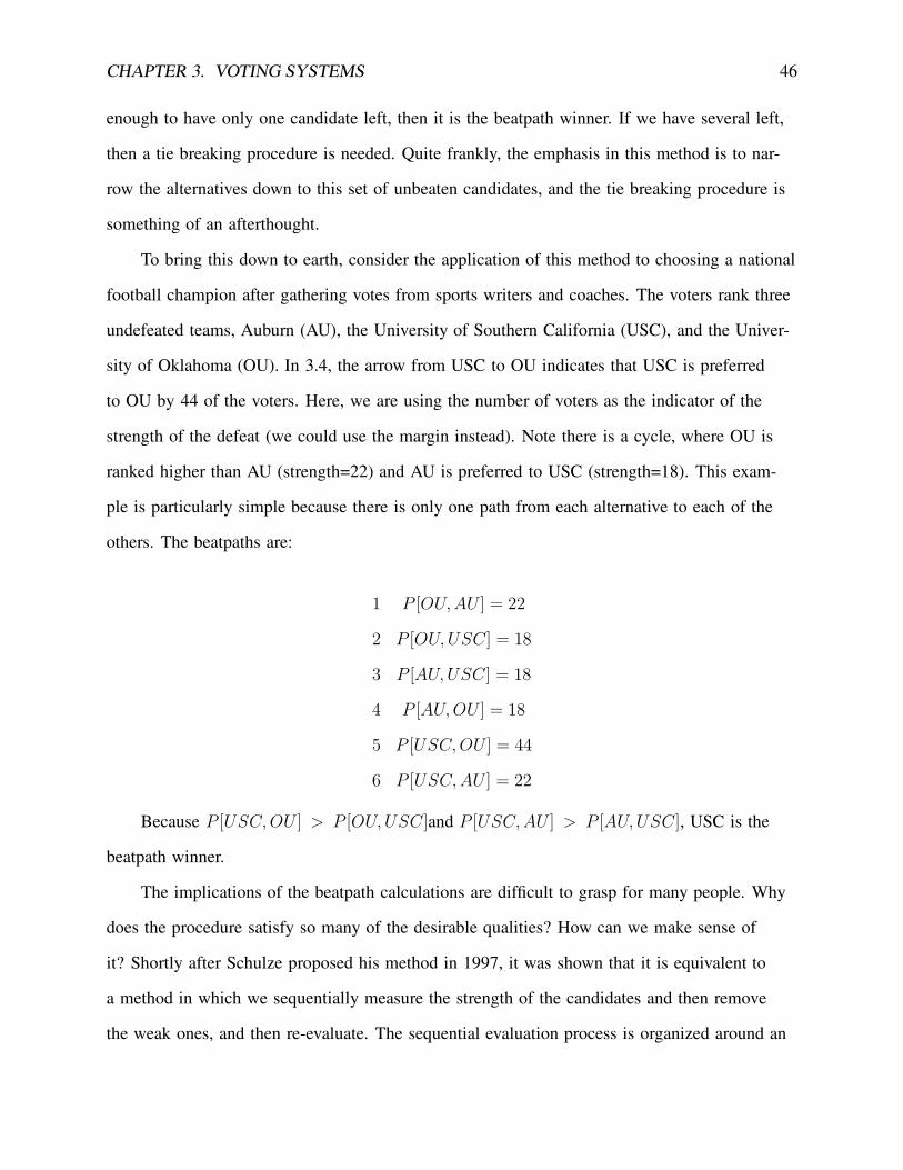
CHAPTER 3. VOTING SYSTEMS 46
enough to have only one candidate left, then it is the beatpath winner. If we have several left,
then a tie breaking procedure is needed. Quite frankly, the emphasis in this method is to nar-
row the alternatives down to this set of unbeaten candidates, and the tie breaking procedure is
something of an afterthought.
To bring this down to earth, consider the application of this method to choosing a national
football champion after gathering votes from sports writers and coaches. The voters rank three
undefeated teams, Auburn (AU), the University of Southern California (USC), and the Univer-
sity of Oklahoma (OU). In 3.4, the arrow from USC to OU indicates that USC is preferred
to OU by 44 of the voters. Here, we are using the number of voters as the indicator of the
strength of the defeat (we could use the margin instead). Note there is a cycle, where OU is
ranked higher than AU (strength=22) and AU is preferred to USC (strength=18). This exam-
ple is particularly simple because there is only one path from each alternative to each of the
others. The beatpaths are:
1 P [OU, AU ] = 22
2 P [OU, USC] = 18
3 P [AU, USC] = 18
4 P [AU, OU ] = 18
5 P [USC, OU ] = 44
6 P [USC, AU ] = 22
Because P [USC, OU ] > P [OU, USC]and P [USC, AU ] > P [AU, USC], USC is the
beatpath winner.
The implications of the beatpath calculations are difficult to grasp for many people. Why
does the procedure satisfy so many of the desirable qualities? How can we make sense of
it? Shortly after Schulze proposed his method in 1997, it was shown that it is equivalent to
a method in which we sequentially measure the strength of the candidates and then remove
the weak ones, and then re-evaluate. The sequential evaluation process is organized around an
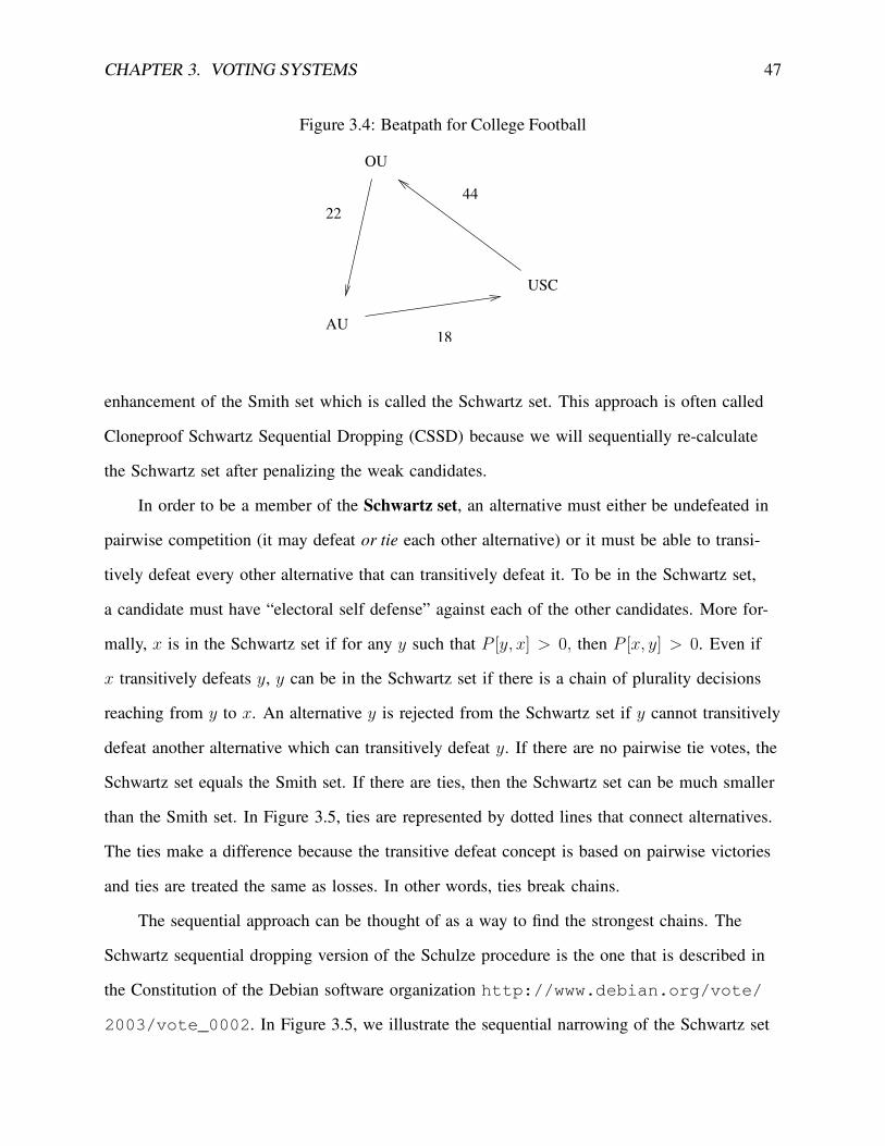
CHAPTER 3. VOTING SYSTEMS 47
Figure 3.4: Beatpath for College Football
USC
AU
OU
4422
18
enhancement of the Smith set which is called the Schwartz set. This approach is often called
Cloneproof Schwartz Sequential Dropping (CSSD) because we will sequentially re-calculate
the Schwartz set after penalizing the weak candidates.
In order to be a member of the Schwartz set, an alternative must either be undefeated in
pairwise competition (it may defeat or tie each other alternative) or it must be able to transi-
tively defeat every other alternative that can transitively defeat it. To be in the Schwartz set,
a candidate must have “electoral self defense” against each of the other candidates. More for-
mally, x is in the Schwartz set if for any y such that P [y, x] > 0, then P [x, y] > 0. Even if
x transitively defeats y, y can be in the Schwartz set if there is a chain of plurality decisions
reaching from y to x. An alternative y is rejected from the Schwartz set if y cannot transitively
defeat another alternative which can transitively defeat y. If there are no pairwise tie votes, the
Schwartz set equals the Smith set. If there are ties, then the Schwartz set can be much smaller
than the Smith set. In Figure 3.5, ties are represented by dotted lines that connect alternatives.
The ties make a difference because the transitive defeat concept is based on pairwise victories
and ties are treated the same as losses. In other words, ties break chains.
The sequential approach can be thought of as a way to find the strongest chains. The
Schwartz sequential dropping version of the Schulze procedure is the one that is described in
the Constitution of the Debian software organization http://www.debian.org/vote/
2003/vote_0002. In Figure 3.5, we illustrate the sequential narrowing of the Schwartz set
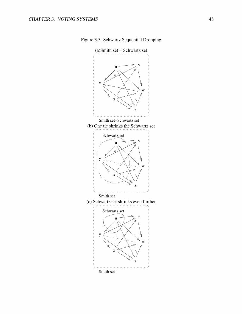
CHAPTER 3. VOTING SYSTEMS 48
Figure 3.5: Schwartz Sequential Dropping
(a)Smith set = Schwartz set
u v
x
y
z
w
Smith set=Schwartz set(b) One tie shrinks the Schwartz set
u v
x
y
z
Schwartz set
Smith set
w
(c) Schwartz set shrinks even further
u v
x
y
z
Schwartz set
Smith set
w
CHAPTER 3. VOTING SYSTEMS 49
that results when ties (dotted lines) are inserted.
Schwartz sequential dropping proceeds iteratively, repeatedly narrowing down the alterna-
tives. It is easy to make this sound more complicated than it really is, but we will try not to.
Step 1. Collect the ranking information from the voters. Voters are allowed to rank all of
the alternatives or just some of them. They are allowed to register their indifference between
alternatives. From the ballots, we can calculate the pairwise outcomes for all alternatives, ei-
ther x �P y or x ≈P y or y �P x.
Now the decision-making starts.
Step 2. Eliminate Rejects. Begin by simplifying the problem by isolating “rejects,” alter-
natives that are losers in the round robin tournament. These losers are the ones that are left
out of the Schwartz set. Recall that y is rejected if it is transitively defeated by some other
proposal and there is no chain that leads from y to that other alternative. The rejects are elimi-
nated from consideration, permanently.
Step 3. Evaluate the remaining contenders (members of the Shwartz set).
A. If there is only one remaining contender, then it is the winner.
B. If there is more than one contender, check the pairwise comparisons among all of the
contenders. If all pairs are tied, it means, in some sense, that we have found all of the alter-
natives that are “equally good.” If all are tied, proceed to the tie-breaking procedure in Step
4.
C. If all contenders are not tied pairwise, then we need to make some changes so we can
reject more alternatives. Here is where the “sequential dropping” kicks in. Among all pairs
of contenders, find the “weakest pairwise defeat.” (To us, a name like “least impressive vic-
tory” would be more fitting.) The idea is to spot the least worthy pairwise victor and demote
it. How to spot the least impressive winner? Look for the alternative that wins with the small-
est number of votes.3 When the weakest pairwise defeat is found, that victory can be erased3Some versions of this procedure use the margin of victory, rather than the absolute number of votes received
by the winner. Schulze recommends the total number of votes because he feels it gives voters a positive incentive toreport their rankings as completely as possible. Otherwise, they might have an incentive to report just the rankings ofthe top one or two alternatives in order to “game” the election system.
CHAPTER 3. VOTING SYSTEMS 50
by changing it to a tie in the data. That is, we change the result in the round robin data for the
weakest defeat from �P to ≈P . (Caution: contrary to what some Web sites say, neither the
weakest defeat nor the tied alternatives are not dropped literally. The weakest defeat is con-
verted to a tie and the Schwartz set is recalculated.) If there are several alternatives that are
equally weak winners–many weakest defeats exist–then choose the one with the most votes for
the loser and declare that one to be the weakest defeat. If there are several pairs tied in both
the number of votes for the winner and the loser, treat them all in the same way: change the
pairwise comparison to a tie. This generates new round robin data.
Go back to Step 2 and repeat the procedure. Use the new round robin data, of course.
The rejects that were eliminated in previous stages are never re-admitted. Since we have in-
serted some ties into the results, the members of the Schwartz set will change: some con-
tenders will become rejects and then they are dropped. The procedure will repeatedly loop
between Steps 2 and 3 until the condition described in Step 3B is obtained.
Step 4. If we arrived at this stage, it means we have narrowed down the alternatives to
the most appealing set of more-or-less equally good outcomes. Schulze calls these “potential
winners.” A winner is selected by a tie breaking rule.
The tie breaking rule that is suggested by Schulze is, more-or-less, going to rank the tied
outcomes by listening to the opinions of randomly drawn voters. Suppose the tied candidates
are {w, x, y, z}. Randomly draw a ballot and copy down the preferences of the voter. If that
ballot states a ranking for all of the alternatives, then that is the end of the procedure. The
group result will match that ballot. If the ballot is only partially filled in, for example, it states
only x �i y, then we take that information and mark down x �Schulze y (it is “set in stone,”
unalterable) and we draw another ballot. If that ballot has preference information about can-
didates that are not already sorted by �Schulze, such as w, and y, then use that information
w �Schulze y. We draw ballots at random until every pairwise comparison is filled in, and we
never change any of the Schulze comparisons we have already completed. If we happen to go
through all ballots without ranking all of the alternatives, then the final ranking is assigned at
CHAPTER 3. VOTING SYSTEMS 51
random.
The Schulze method can be applied to any of the voting examples we have considered. Of
course, if the preferences imply the existence of a Condorcet Winner, then that alternative is
chosen and the solution is simple. To find a more interesting case, we need to select an exam-
ple in which there is a voting cycle. Recall the Borda paradox considered in section 3.4.2. In
Figures 3.6 and 3.7, we have used the preferences from Tables 3.3 and 3.4 with the Schwartz
sequential dropping approach.
In Figure 3.6, we note that the original preferences allow a majority rule cycle across all
of the alternatives, so the first stage Schwartz set includes all of the alternatives. There are two
comparisons tied for the weakest defeat, each with the support of 4 voters, so in 3.6b, those
arrows are changed to dotted lines representing ties. After those ties are taken into account, the
Schwartz set is recalculated, and it includes only w.
Recall that alternative z is exposed as a fraud in that example. The effect of dropping z to
the bottom of the voter preference orderings appears in 3.7. Note that the initial Schwartz set
now includes three alternatives, {w, x, y}. Alternative z is excluded (it is a Condorcet loser).
The weakest defeat is between w and y. After that is changed to a tie, then w is the only po-
tential winner remaining. The same alternative, w, wins with the Schulze method in both cases.
The Schulze method has the apparent strength of solving the paradox in the Borda count:
w wins in both cases. The Schulze method is thus more stable and, in some sense, more log-
ical. The fact that the Borda method chose y in the original example (Table 3.3) and Schulze
chooses w deserves mention. From a beatpath point of view, it appears that we did not cor-
rectly understand the Borda problem in section 3.4.2. We thought the paradox was that y was
turned from a winner into a loser when the fortunes of z changed. Now it appears that the
original Borda winner, y, was “wrong.” Borda chose the wrong winner because it allowed z
to play the role of a spoiler, somehow distracting voters from their purpose, thus allowing y to
win. When z is moved to the bottom in Table 3.4, its role (its influence as an irrelevant alter-
native) is eliminated, and the “correct alternative” w wins.

CHAPTER 3. VOTING SYSTEMS 52
Figure 3.6: Schulze Method Applied to Table 3.3
(a) Pairwise comparisons
4
5x
y7
5
5
z
w
4
Schwartz set
(b) Change weakest defeats to ties5
x
y7
5
5
z
w
(c) Second-stage Schwartz set includes only w
5x
y7
5
5
z
w
Schwartz set
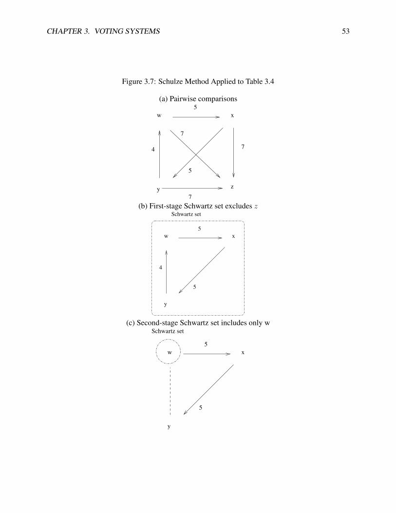
CHAPTER 3. VOTING SYSTEMS 53
Figure 3.7: Schulze Method Applied to Table 3.4
(a) Pairwise comparisons
4
5x
y7
7
5
z
w
7
(b) First-stage Schwartz set excludes z
4
5x
y
5
w
Schwartz set
(c) Second-stage Schwartz set includes only w
5x
y
5
w
Schwartz set
CHAPTER 3. VOTING SYSTEMS 54
The Schulze method leads to a full, transitive ordering of all of the candidates. The beat-
path values P [x, y] can be used to sort alternatives from top to bottom. As a result, the method
could be used to determine the winner of the Division 1A College football championship on
the basis of the rankings submitted by coaches, writers, or computers.
The reader might be wondering, “if this method is so great, why isn’t everyone using it?”
Well, if you ask its proponents, we expect they will say “because everyone is not very smart!”
Ordinary people–not academics–are not particularly interested in election procedures, much
less complicated ones. As a result, the most widely used argument against the method seems
to be that it is too complicated. To academics, this is not a very good argument, but it carries
a lot of weight with real life policy makers. In response, the Schulze proponents will point out
that, from a voter’s point of view, it is no more complicated than a Borda count. All the voters
need to do is submit rankings of some alternatives. The counting process is more complex, of
course, but the effort is justified. The proponents can list a long list of favorable qualities that
we have already mentioned, plus some more.
The beatpath approach is not completely free from the anomalies that infect the other vot-
ing mechanisms. Schulze draws our attention to the fact that his method violates the Partic-
ipation Criterion. The participation criterion says that if an election has been decided, and
then you add voters who prefer the winner to another alternative, then adding those new vot-
ers must not result in the victory of that other (less favored) alternative. More formally, the
winner is x, hence socially x �Schulze y. Add more voters such that x �i y. Adding those
voters should not change the social result to y �Schulze x. The criterion does not require that
x must still win, only that adding voters who do not prefer y should not make y the winner.
Please note that the participation criterion is different from the monotonicity principle. Mono-
tonicity states that among existing voters, a change in voter preferences that favors x against y
must not hurt x’s position in the final decision. Participation concerns the addition of new vot-
ers. Schulze is a monotonic procedure, but examples can be found to show that it violates the
participation criterion.
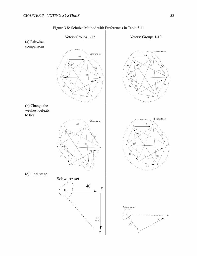
CHAPTER 3. VOTING SYSTEMS 55
Figure 3.8: Schulze Method with Preferences in Table 3.11
Voters:Groups 1-12 Voters: Groups 1-13(a) Pairwisecomparisons
u v
wx
yz
40
42
32
38
36
36
Schwartz set
38
34
u
wx
yz
43
42
35
3339
3336
3341
3833
33
34
33
33
Schwartz set
v
(b) Change theweakest defeatsto ties
u v
wx
yz
40
42
38
36
36
Schwartz set
38
34
u v
wx
yz
43
42
35
39
36
41
38
34
Schwartz set
(c) Final stage
u v40Schwartz set
z
38wx
y
42
41
Schwartz set
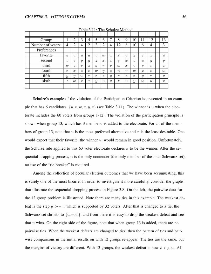
CHAPTER 3. VOTING SYSTEMS 56
Table 3.11: The Schulze Method
Group: 1 2 3 4 5 6 7 8 9 10 11 12 13Number of voters: 4 2 4 2 2 2 4 12 8 10 6 4 3
Preferencesfavorite u u u u v w w x y z z z u
second v v y y z x x y w u u y y
third w z v z u v v w x v v x z
fourth x x z v w y z u v w x v w
fifth y y w w x z y v z x y w v
sixth z w x x y u u z u y w u x
Schulze’s example of the violation of the Participation Criterion is presented in an exam-
ple that has 6 candidates, {u, v, w, x, y, z} (see Table 3.11). The winner is u when the elec-
torate includes the 60 voters from groups 1-12 . The violation of the participation principle is
shown when group 13, which has 3 members, is added to the electorate. For all of the mem-
bers of group 13, note that u is the most preferred alternative and x is the least desirable. One
would expect that their favorite, the winner u, would remain in good position. Unfortunately,
the Schulze rule applied to this 63 voter electorate declares x to be the winner. After the se-
quential dropping process, u is the only contender (the only member of the final Schwartz set),
no use of the “tie breaker” is required.
Among the collection of peculiar election outcomes that we have been accumulating, this
is surely one of the most bizarre. In order to investigate it more carefully, consider the graphs
that illustrate the sequential dropping process in Figure 3.8. On the left, the pairwise data for
the 12 group problem is illustrated. Note there are many ties in this example. The weakest de-
feat is the step y �P z which is supported by 32 voters. After that is changed to a tie, the
Schwartz set shrinks to {u, v, w}, and from there it is easy to drop the weakest defeat and see
that u wins. On the right side of the figure, note that when group 13 is added, there are no
pairwise ties. When the weakest defeats are changed to ties, then the pattern of ties and pair-
wise comparisons in the initial results on with 12 groups re-appear. The ties are the same, but
the margins of victory are different. With 13 groups, the weakest defeat is now v �P w. Af-
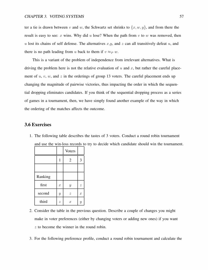
CHAPTER 3. VOTING SYSTEMS 57
ter a tie is drawn between v and w, the Schwartz set shrinks to {x, w, y}, and from there the
result is easy to see: x wins. Why did u lose? When the path from v to w was removed, then
u lost its chains of self defense. The alternatives x,y, and z can all transitively defeat u, and
there is no path leading from u back to them if v ≈P w.
This is a variant of the problem of independence from irrelevant alternatives. What is
driving the problem here is not the relative evaluation of u and x, but rather the careful place-
ment of u, v, w, and z in the orderings of group 13 voters. The careful placement ends up
changing the magnitude of pairwise victories, thus impacting the order in which the sequen-
tial dropping eliminates candidates. If you think of the sequential dropping process as a series
of games in a tournament, then, we have simply found another example of the way in which
the ordering of the matches affects the outcome.
3.6 Exercises
1. The following table describes the tastes of 3 voters. Conduct a round robin tournament
and use the win-loss records to try to decide which candidate should win the tournament.
Voters
1 2 3
Ranking
first x y z
second y z x
third z x y
2. Consider the table in the previous question. Describe a couple of changes you might
make in voter preferences (either by changing voters or adding new ones) if you want
z to become the winner in the round robin.
3. For the following preference profile, conduct a round robin tournament and calculate the
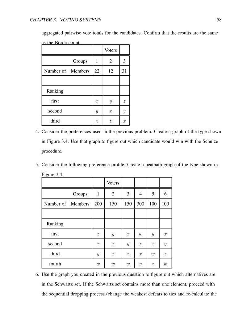
CHAPTER 3. VOTING SYSTEMS 58
aggregated pairwise vote totals for the candidates. Confirm that the results are the same
as the Borda count.Voters
Groups 1 2 3
Number of Members 22 12 31
Ranking
first x y z
second y x y
third z z x
4. Consider the preferences used in the previous problem. Create a graph of the type shown
in Figure 3.4. Use that graph to figure out which candidate would win with the Schulze
procedure.
5. Consider the following preference profile. Create a beatpath graph of the type shown in
Figure 3.4.
Voters
Groups 1 2 3 4 5 6
Number of Members 200 150 150 300 100 100
Ranking
first z y x w y x
second x z y z x y
third y x z x w z
fourth w w w y z w
6. Use the graph you created in the previous question to figure out which alternatives are
in the Schwartz set. If the Schwartz set contains more than one element, proceed with
the sequential dropping process (change the weakest defeats to ties and re-calculate the
CHAPTER 3. VOTING SYSTEMS 59
Schwartz set).
7. This is a challenging problem, one which we refer to in the feature box on 43. Show
that if the Borda count (or, equivalently, the aggregated pairwise vote) outcome is x �AP
y ≈AP z, then the only pairwise outcomes that are consistent with that outcome are the
ones listed in equation 3.8.
3.7 Single Vote Systems: Cousins of Plurality and Majority
Rule
We began this chapter with the plurality problem. A plurality election with twenty or thirty
candidates might award victory to a very unpopular candidate. The poster children for the
problem might be the Democratic and Republican candidates in Minnesota’s gubernatorial
election who were edged-out by Jesse Ventura. In the words of mathematician Keith Devlin,
Jesse Ventura “won not because the majority of the voters chose him, but because plurality
voting effectively thwarted the will of the people. Had the voters been able to vote in such
a way that, if their preferred candidate were not going to win, their preference between the
remaining two would be counted, the outcome would have been quite different” (2004). The
alternative schemes, the Borda rank order voting plan and the pairwise Condorcet systems, of-
fer some hope. They have not won the hearts and minds of electoral reformers with the same
power as the alternative to which we now turn our attention.
This system requires the voters to come to the polls only once. The voters rank the alter-
natives and then the election officials can proceed “as if” there really were a run-off election.
When this procedure is used to select a single winner in an election, it is generally referred to
as an Instant Runoff Vote (IRV) or an Alternative Vote system. When the method is used to
select a group of candidates, such as the top 5 nominees for the Grammy Awards, or in a pro-
portional legislative election, the procedure is called the Single Transferable Vote (STV). The
CHAPTER 3. VOTING SYSTEMS 60
procedures are the same for choosing a single winner, but the details get complicated for se-
lecting the additional winners. There are two prominent implementations of the STV concept,
the Hare system (in honor of Thomas Hare, an English proponent of this system), the Hare-
Clark system (add an honorific for Andrew Inglis Clark, a Tasmanian Attorney-General who
pushed a variant of the STV into usage). The transferable vote is in use in national elections
in Australia, Malta and Ireland as well as in local elections in Cambridge, Massachusetts, San
Francisco, California, and cities in Northern Ireland, and New Zealand. The method is used in
faculty elections at Cornell University.
We will focus our attention on the selection of a single winner from a field of candidates,
so we will detail only that part of the procedure.
The winner must obtain a target number of votes, dubbed the quota. If there is only one
spot open–only one candidate can win–the usual quota is the majority of the votes:
quota = majority ≥Number of voters + 1
2
On election day, the voters go to the polls and rank the candidates from first to last in
order of desirability. Then election managers name the winner by applying the following algo-
rithm.
Step 1. A voter’s support on the first ballot is given to the voter’s top-ranked candidate.
If one of the candidates has a majority, then that candidate is the winner. If no candidate has a
majority, proceed to Step 2.
Step 2. The candidate with the smallest number of votes is eliminated from consideration.
The ballots of the voters who had supported that eliminated candidate are reconsidered. Their
votes are transferred to their second-ranked candidates. Then the votes are re-tabulated. If a
candidate has a majority, then it is declared the winner. Otherwise, repeat Step 2. (The candi-
date that was eliminated in this step is excluded throughout the remainder of the process.)
If the election is choosing 5 members of a commission or a legislative delegation, the pro-
CHAPTER 3. VOTING SYSTEMS 61
cedure is slightly more involved. Not only are the votes cast for the losers transferred, but also
the “excess” votes (ones which exceed the quota) received by the winners can be transferred.4 The calculations in that re-allocation are a bit involved; that is where the variants of STV
diverge. The main idea in the procedure is that candidates are removed one-by-one, and the
votes cast for the removed candidates are either counted for them (as part of their quota) or
transferred and counted for other candidates that the voter also supports.
The proponents of this method claim that it does not throw away information in the same
way as a plurality election. It saves voters from the terrible choice that is forced on them by
a plurality vote. If the voters who favor either the Democrat or the Republican against Jesse
Ventura have a chance to declare that priority, then Ventura might not end up winning in the
Instant Runoff. The “Ventura problem,” coupled with the on-going use of the procedure in
some places, gives the STV advocates some persuasive ammunition. Krist Novoselic, most
well known as a member of the band Nirvana, has written a book that combines his band
memoir with an endorsement of transferable votes, Of Grunge and Government: Let’s Fix This
Broken Democracy (2004). He also hosts a website (http://www.fixour.us). He eagerly watched
the introduction of STV in San Francisco for the 2004 Board of Supervisors elections. Steven
Hill, of the Center for Voting and Democracy, a proponent of the transferable vote systems, en-
thusiastically proclaimed, “More voters picked their supervisor, and fast results mean that San
Francisco avoided a December runoff election, saving millions in taxes (the cost of the second
election)”(Novaselic, 2004).
There is no doubt that the STV might work to correct bad outcomes in some particular
examples. Perhaps Jesse Ventura might not have been governor of Minnesota. There are ex-
ample problems that we can consider in which the STV does not seem to perform too badly.
If the STV procedure is applied to the preferences of groups 1-12 in Table 3.11 (the data for
the Schulze example that violated the participation criterion), the STV stages eliminate v, then4
quota =Number of votes cast
Number of winners to be chosen + 1+ 1
Note that if there is one winner to be chosen, the winner must have a bare majority.
CHAPTER 3. VOTING SYSTEMS 62
w, then y, and then u. The two remaining candidates, x and z, are tied with 30 votes. After
adding group 13 into the calculations, the elimination process rejects the alternatives in the
same order (v, w, y, and then u). The winner is z, which earns 33 votes against the 30 for x.
The new voters prefer z to x, and it seems quite reasonable that adding them to the electorate
would tip the scales in favor of z.
On the other side of the ledger, however, the STV has several properties that should cause
concern. The fact that the STV system does not always select a Condorcet Winner (when one
exists) is a serious shortcoming. Academic research has often concentrated on another issue:
STV is not monotonic. The principle of monotonicity has first come to our attention in the
consideration of majority rule and May’s Theorem. Now it comes to the forefront again. The
basic idea of the Monotonicity Criterion is that an election system should be responsive, and
not in a perverse way. If a voter changes his mind and decides to rank an alternative more
highly, then that alternative’s electoral fortunes should be helped, or at least not hurt. This is
the property commonly called weak monotonicity.
Consider the preference rankings in Table 3.12. There are preferences for five groups,
{1, 2, 3, 4, 5} and four alternatives, {w, x, y, z}. The STV algorithm proceeds as follows.
1. The first place votes are, in order, w=9, x=6, y=6, z=5.
2. Eliminate z, so the candidates are w, x and y. Re-allocate the votes of group 1 to their
second-ranked candidate, x. The votes are retabulated: x=11, w=9, y=6.
3. Eliminate y, so the final 2 candidates are w and x. Reallocate the votes of groups 2
and 3 to x. The final vote totals are x=17, w=9. So x is declared the winner.
We make only one small change in order to demonstrate the fact that STV is nonmono-
tonic. We will replace group 3 with the voters in group 3′, so that the columns being used in
the vote are {1, 2, 3′, 4, 5}. We hope the reader will agree that this seems to be an innocuous
change. The voters in 3 think x is second best, but the voters in 3′ think that x is the most de-
sirable of all; x should still win, shouldn’t it?
Observe how the STV result changes.
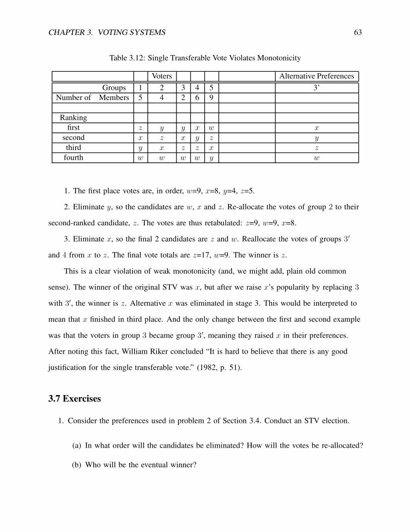
CHAPTER 3. VOTING SYSTEMS 63
Table 3.12: Single Transferable Vote Violates Monotonicity
Voters Alternative PreferencesGroups 1 2 3 4 5 3’
Number of Members 5 4 2 6 9
Rankingfirst z y y x w x
second x z x y z y
third y x z z x z
fourth w w w w y w
1. The first place votes are, in order, w=9, x=8, y=4, z=5.
2. Eliminate y, so the candidates are w, x and z. Re-allocate the votes of group 2 to their
second-ranked candidate, z. The votes are thus retabulated: z=9, w=9, x=8.
3. Eliminate x, so the final 2 candidates are z and w. Reallocate the votes of groups 3′
and 4 from x to z. The final vote totals are z=17, w=9. The winner is z.
This is a clear violation of weak monotonicity (and, we might add, plain old common
sense). The winner of the original STV was x, but after we raise x’s popularity by replacing 3
with 3′, the winner is z. Alternative x was eliminated in stage 3. This would be interpreted to
mean that x finished in third place. And the only change between the first and second example
was that the voters in group 3 became group 3′, meaning they raised x in their preferences.
After noting this fact, William Riker concluded “It is hard to believe that there is any good
justification for the single transferable vote.” (1982, p. 51).
3.7 Exercises
1. Consider the preferences used in problem 2 of Section 3.4. Conduct an STV election.
(a) In what order will the candidates be eliminated? How will the votes be re-allocated?
(b) Who will be the eventual winner?
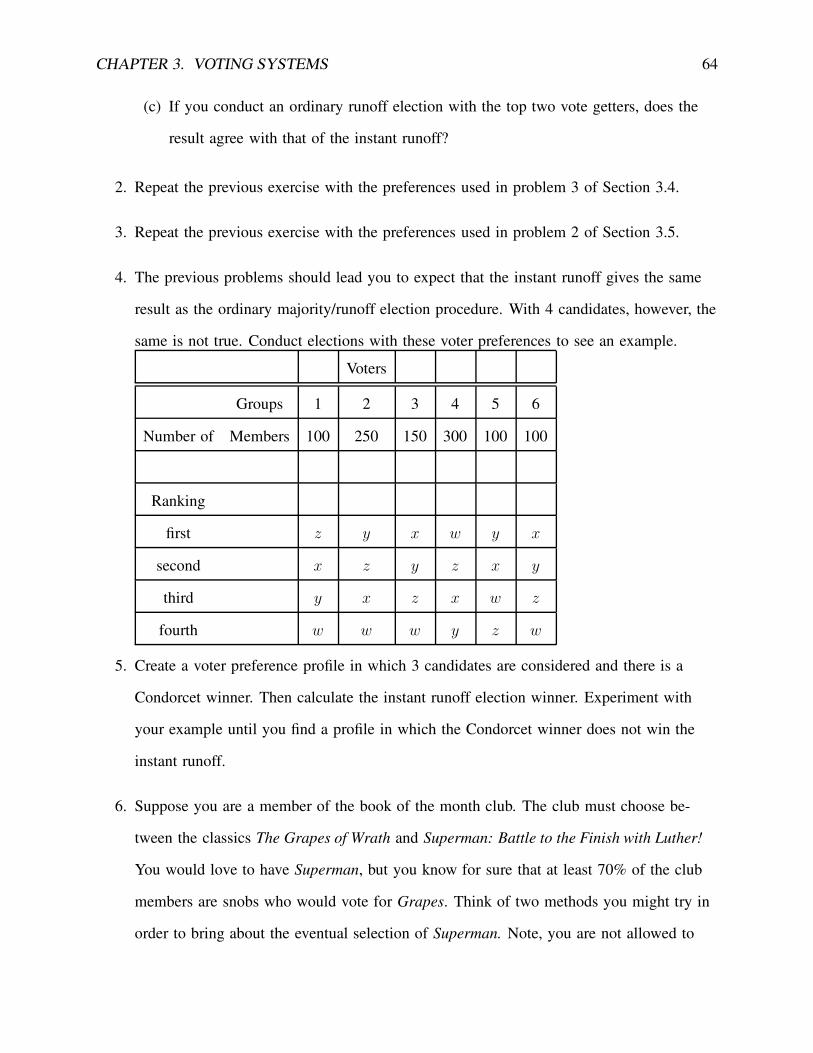
CHAPTER 3. VOTING SYSTEMS 64
(c) If you conduct an ordinary runoff election with the top two vote getters, does the
result agree with that of the instant runoff?
2. Repeat the previous exercise with the preferences used in problem 3 of Section 3.4.
3. Repeat the previous exercise with the preferences used in problem 2 of Section 3.5.
4. The previous problems should lead you to expect that the instant runoff gives the same
result as the ordinary majority/runoff election procedure. With 4 candidates, however, the
same is not true. Conduct elections with these voter preferences to see an example.
Voters
Groups 1 2 3 4 5 6
Number of Members 100 250 150 300 100 100
Ranking
first z y x w y x
second x z y z x y
third y x z x w z
fourth w w w y z w
5. Create a voter preference profile in which 3 candidates are considered and there is a
Condorcet winner. Then calculate the instant runoff election winner. Experiment with
your example until you find a profile in which the Condorcet winner does not win the
instant runoff.
6. Suppose you are a member of the book of the month club. The club must choose be-
tween the classics The Grapes of Wrath and Superman: Battle to the Finish with Luther!
You would love to have Superman, but you know for sure that at least 70% of the club
members are snobs who would vote for Grapes. Think of two methods you might try in
order to bring about the eventual selection of Superman. Note, you are not allowed to
CHAPTER 3. VOTING SYSTEMS 65
make a persuasive speech to change their minds or do anything that would change the
pairwise comparison of the two books, but you can introduce new alternatives and differ-
ent voting methods.
3.8 Conclusion
After reviewing the many voting systems and studying the many principles by which they are
judged, the reader has a right to ask the author, “how do you rank these systems? Which is the
best?”
We find ourselves wishing that there were some voting system that would meet all of the
requirements that seem fair and logical. Wishing does not make it so, sadly enough. In fact,
there is a theorem, known as Arrow’s Possibility Theorem, which states, basically, that it is
mathematically impossible to find a voting system that satisfies what appear to be the most
basic, bare-minimum requirements. Arrow, an economist, was awarded the Nobel prize, partly
on the basis of this research (Arrow, 1963).
Arrow’s theorem can be stated in several ways. We think this is the most useful version.
Suppose there is an election ranking system that meets these requirements:
Nondictatorial The social ranking does not mirror the tastes of one voter i without regard to
the tastes of the other voters.
Pareto Principle If all voters favor one alternative over another, then the social ranking should
respect that and rank the alternatives accordingly.
These seem like such simple, fundamental elements that they can be assumed as necessary in-
gredients in a social ranking procedure. Arrow’s Possibility Theorem says the following. If an
election system is nondictatorial and obeys the Pareto principle, then it is possible to find an
example set of voter preferences such that:
1. The social ranking is intransitive (a voting cycle), and/or
CHAPTER 3. VOTING SYSTEMS 66
2. Independence of irrelevant alternatives (IIA) is violated.
It is very important to emphasize that the Possibility Theorem does not mean that a rank-
ing procedure is always intransitive or in violation of IIA. Rather, it is always possible to find
an example society, a set of voter preferences, such that the result is somehow illogical. If the
result is intransitive, then we have the paradox of “rational man, irrational society”(Barry and
Hardin, 1982). If we adopt a system that blocks intransitivity, such as the Borda count, then
we know for sure there are examples in which independence from irrelevant alternatives is vio-
lated.
Arrow’s theorem is sometimes overstated. For example, some students think it says that
democracy is always illogical. It does not mean anything of the kind. Rather, it means that it
is not possible to find a democratic procedure that works in a sensible way all of the time.
If it is not possible to meet such basic, simple criteria as nondictatorship, of course it is
not possible to meet even more elaborate properties like the participation criterion. As a result,
the choice of electoral system has to be based not on which system meets all of the specified
criteria, but rather on a value judgment about what sorts of peculiarities are the most harmful
and which sorts of societal preference profiles are most likely to arise and cause peculiarities.
If the reader wants to know “which ranking system is best?” we can sympathize. We
want to know the same thing. And so do most political scientists, economists, mathematicians,
physicists, and psychologists.
Personally speaking, we have found a pleasant results by using procedures that elimi-
nate the obviously bad candidates (by some principle like the Smith set or the Schwartz set)
and then choosing among the remainder by a positional method like the Borda count or the
Schulze method. We have been very unhappy with decisions reached by pure plurality or a
runoff election. The STV might be preferable to a plurality or majority rule election, but the
fact that it is so badly nonmonotonic causes us to shy away from it. That is to say, plurality
rule is truly bad, as both Borda and Condorcet had contended, and we would rather have STV
than plurality, but we’d rather have one of the more elaborate two-stage procedures instead of
CHAPTER 3. VOTING SYSTEMS 67
either one.
Suggested Readings
Readers who look into this further will no doubt find ten or twenty seriously proposed
election procedures, all of which have advantages worth considering. Perhaps one would begin
with the textbook by William Riker (1982) and then do some soaking and poking in the Inter-
net. We have found many fascinating Web sites and would encourage readers to adventure, but
keep in mind that these sites are not peer reviewed by experts and we have noticed a nontrivial
number of mistakes in interpretation and mathematics. Perhaps the most rigorous analysis is to
be found on the election-methods email list, which is hosted on http://electorama.com.
Bibliography
Arrow, Kenneth. 1963. Social Choice and Individual Values, 2ed. Wiley.
Barry, Brian W. and Russell Hardin. 1982. Rational Man and Irrational Society? An Introduc-
tion and Sourcebook. Beverly Hills: Sage Publications.
Bauer, Alissa. December 8, 2004. “Rank System Strips Teams of Postseason Opportunities.”
University Daily Kansan .
Black, Duncan. 1958. The Theory of Committees and Elections. Cambridge: Cambridge Univer-
sity Press.
de Borda, Jean-Charles. 1781. Mémoire sur les Élections au Scrutin’. Paris: Histoire del
l’Académie Royale des Sciences.
de Condorcet, Marquis. 1785. Éssai sur L’application L’analyse à la probabilité des dés Déci-
sions Rendues à la Pluralité des Voix (trans. Essay on the Application of Mathematics to the
Theory of Decision-Making). Paris.
Devlin, Keith. 2004. “Election Math.” Devlin’s Angle, MAA Online .
URL http://www.maa.org/devlin/devlin_114_04.html
Fishburn, Peter C. 1974. “Paradoxes of Voting.” American Political Science Review 68(2):537–
556.
Harsanyi, John C. 1955. “Cardinal Welfare, Individualistic Ethics, and Interpersonal Compar-
isons of Utility.” Journal of Political Economy 61:309–321.
68
BIBLIOGRAPHY 69
Hilburn, Robert. February 28, 2002. “It’s Time to Nominate a New System.” Los Angeles
Times .
Johnson, Paul E. 1998. Social Choice: Theory and Research. Thousand Oaks, CA: Sage.
Jones, Bradford, Benjamin Radcliffe, Charles Taber, and Richard Timpone. 1995. “Condorcet
Winners and the Paradox of Voting.” American Political Science Review 89(1):137–144.
Mackenzie, Dana. 2000a. “Making Sense Out of Consensus: How Did That Guy Win?” SIAM
News 33.
Mackenzie, Dana. 2000b. “May the Best Man Lose.” Discover .
May, Kenneth O. 1952. “A Set of Independent Necessary and Sufficient Conditions for Simple
Majority Decision.” Econometrica 20:680–784.
Nash, John F. 1950. “The Bargaining Problem.” Econometrica 18:155–162.
Nelson, Randy A., Michael R. Donihue, Donald M. Waldman, and Calbraith Wheaton. 2001.
“What’s An Oscar Worth?” Economic Inquiry 39(1):1–16.
Novaselic, Krist. 2004. “Instant Runoff Voting Used for First Time in San Francisco Elec-
tions.” http://www.fixour.us/editorials/11.08.04.html.
URL http://www.fixour.us/editorials/11.08.04.html
Novoselic, Krist. 2004. Of Grunge & Government: Let’s Fix This Broken Democracy! Akashic
Books.
Reilly, Benjamin. 2002. “Social Choice in the South Seas: Electoral Innovation and the Borda
Count in the Pacific Island Countries.” International Political Science Review 23(4):355–372.
Riker, William H. 1982. Liberalism Against Populism: A Confrontation Between the Theory of
Democracy and the Theory of Social Choice. San Francisco, CA: W. H. Freeman.
BIBLIOGRAPHY 70
Riker, William H. 1986. The Art of Political Manipulation. New Haven, CT: Yale University
Press.
Saari, Donald G. 1994. Geometry of Voting. Berlin: Springer-Verlag.
Schulze, Markus. 2003. “A New Monotonic and Clone-Independent Single-Winner Election
Method.” Voting Matters 17:9–19.
Woodling, Chuck. December 24, 2004. “Maybe It’s Time To Do Away with AP Poll.”
Lawrence Journal World page 3C.

![Chapter 2 Review Name: Class Pd. Chapter 2 Weighted Voting ... · Chapter 2 Weighted Voting Systems: ... In the weighted voting system [q: 30, 29, 16, 8, 3, 1] a two-thirds majority](https://img.pdfslide.us/doc/110x75/5abfcb967f8b9aa15e8e7214/chapter-2-review-name-class-pd-chapter-2-weighted-voting-2-weighted-voting.jpg)