Chapter 3 THERMODYNAMICS: A BRIEF SUMMARYharris/thermo.pdf · Chapter 3 THERMODYNAMICS: A BRIEF SUMMARY 1. PREAMBLE Although many of the systems usually addressed in thermodynamics

Chapter 3

THERMODYNAMICS: A BRIEF SUMMARY

1. PREAMBLE

Although many of the systems usually addressed in thermodynamicsand statistical mechanics are identical, these two disciplines are distin-guished by their methodology. A system in statistical mechanics is de-fined by specifying its microscopic Hamiltonian, from which, at least inprinciple, one can obtain the energy levels of the system and, by apply-ing the machinery of statistical mechanics, one can evaluate experimen-tally observable quantities, which include not only macroscopic responsefunctions, but also space- and time-dependent correlation functions. Incontrast thermodynamics takes a completely macroscopic and phenom-enological approach to describing systems. A system in thermodynamicsis defined by specifying the small number of thermodynamic variables(e. g. pressure, temperature, and volume) needed to characterize thesystem. As we shall see the macroscopic properties of such a system areobtainable from a thermodynamic potential (e. g. the internal energyor the free energy) when these potentials are expressed in terms of theircorrect variables. This last statement applies to both thermodynamicsand statistical mechanics, and, in fact, the latter provides the means forcalculating these potentials from the underlying microscopics

In this section we summarize those aspects of thermodynamics whichwill be most relevant for our study of statistical mechanics. So ouraim is relevance rather than completeness. We assume the student hasbeen exposed to an undergraduate course on thermodynamics. If thisassumption is incorrect, the student is advised to refer to one or more ofthe standard undergraduate texts on thermodynamics, such as the oneby H.Callen.

D R A F T January 13, 2001, 7:05am D R A F T

30 STATISTICAL MECHANICS

We remind the reader of what we consider to be a very surprisingand striking fact, namely that although thermodynamics is based on anumber of seemingly innocuous observations about how matter behavesand comes to equilibrium, it nevertheless gives rise to rather nontrivialrelations between observables. Also we must keep in mind the fact thatstatistical mechanics must be consistent with, and hopefullly elucidateand explain, thermodynamics. In what follows we will occationally notethe connection between the macroscopic description of thermodynamicsand the microscopic description of statistical mechanics.

2. THE LAWS OF THERMODYNAMICSThermodynamics concerns itself with systems, like those discussed in

the introductory chapters, which are characterized by a small numberof macroscopic variables. Thermodynamics does not specify the numberand choice of these variables. Their choice is dictated by the systemunder consideration. For instance for liquid systems the variables arepressure p, volume V , temperature T , and the amount of material asspecified by the number of particles, N or the number of moles n. Ifthree of these quantities are fixed, then the other is determined. Formagnetic systems one may select three independent variables out of theset M , the total magnetic moment of the system, H, the applied field(which we assume to be uniform in space and time), T and n. Thecrucial point is that for any given system, the number of independentvariables is fixed by the nature of the system and can not be inferredfrom thermodynamic considerations.

We will restrict our attention to systems which are in, or very nearlyin, equilibrium. This means that these systems have had time to relaxso that their thermodynamic variables are not changing with time. Bycommon consent, there are four Laws of Thermodynamics. We nowstudy these in turn.

2.1 THE ZEROTH LAW OFTHERMODYNAMICS

We start with what is called the Zeroth Law of Thermodynamics.This law concerns the nature of equilibrium and establishes the conceptof temperature. Consider the result when two systems, A and B, eachof fixed volume come to equilibrium under the condition that they areallowed to interact weakly and exchange energy. The Zeroth Law ofThermodynamics says that if system A is in equilibrium with both sys-tems B and C, then B and C are in equilibrium with each other. Thissatement implies that when systems B and C are brought into thermal


Thermodynamics: a brief summary 31

contact with one another, none of their properties change. That resultis the signal that they were already in equilibrium with one another. Asa consequence of the Zeroth Law it is possible to assign a parameter, theempirical temperature, θ, to these systems such that two systems havingthe same value of θ, are in thermal equilibrium with each other. Thisformulation therefore implies an obvious conclusion from our experience:if system A has the same temperature (on any scale of temperature) assystems B and C, then the temperatures of B and C (on any scale oftemperature) will be the same. This knowledge, in itself, provides nometric or indeed any ordering of empirical temperature. At this point,the concept that one body is hotter than another is not yet introducedor implied. One of the first steps in statistical mechanics is to identifyhow the concept of temperature arises.

2.2 THE FIRST LAW OFTHERMODYNAMICS

Before discussing the First Law of Thermodynamics we remind thereader of a philosophical conundrum concerning the famous equationF = ma. One might imagine interpreting this law as meaning that, afterwe define m and a, this equation then provides a definition of force, whichis not otherwise defined. This point of view is certainly not normallyused in teaching first year students. However, if this were the end ofthe story, then Newton’s Second Law would not be as useful as it is. Itis useful because we also have independently defined forces, such as themutual repulsion of two like charges, or the force generated for a givenextension of a spring. Then F = ma becomes an equation with content,relating three previously defined quantities. A similar dichotomy alsoappears in the discussion of the First Law, which is written as

dU = ∆Q + ∆W , (3.1)

where ∆W is the work done on the system, ∆Q is the heat added tothe system, and dU is the increase in the system’s internal energy. (Themeaning of ∆ as contrasted to d in Eq. (3.1) will become clear in amoment.) The most traditional approach to discussing this equation isto say that this equation defines what heat is. It is what is left over afteryou have calculated the work done and taken account of the change ininternal energy of the system. In this context, there is general agreementon how the work done on a system is to be defined. If a piston is movedinward through a distance dx by a force F , then the work done on thesystem is Fdx. The question, of course, is whether or not this quantitycan be related to parameters pertaining to the system enclosed by thepiston. indeed, if the work is done quasistatically and reversibly, then



we may write, for the liquid-gas system

∆W = −pdV , (3.2)

where, since the process is accomplished via a sequence of equilibriumstates, we may take p to be the equilibrium pressure. In the homework,corrections to Eq. (3.2) are discussed when work is done near the qua-sistatic limit. In the next section we will discuss work in electric andmagnetic systems.

To give content to Eq. (3.1) we define heat calorimetrically as follows.One unit of heat is the energy that leaves a standard body when its em-pirical temperature (on some specific scale) is decreased from a standardvalue T0 by some fixed amount ∆T without doing any work. In principle,rational fractions of units of heat can be established by transferring heatbetween integer multiples of identical systems. (At this point we wouldnot want to define half a unit of heat in terms of a change in temperature∆T/2 because we have not yet established a metric for temperature.)Then by transferring heat between systems (which may be at quite dif-ferent temperatures) without performing any work, one can establishof scale of heat transfer, at least in simple contexts. To define heat ina general situation will involve comparing the effect of some operationto that of calorimetrically transferring heat. For instance, to define theheat transferred when a flame is applied to a body when no work is doneon the body, one would compare the effect of the flame to a calorimetricapplication of heat.

Thus, for any process, we have defined the heat added to a system ∆Qand the work ∆W done on the system. Notice that these quantities arenot differentials of heat and work functions. In particular, to establishthat some quantity, X, is a function of thermodynamic variables (such afunction is called a “state function”) we would have to prove that, whena system is taken around a path which begins and ends at the same ther-modynamic state, the path integral

∮dX vanishes. This is clearly is not

the case with ∆Q or ∆W , as is illustrated in the homework. The FirstLaw of Thermodynamics says that although ∆W and ∆Q are themselveseach not differentials of state functions, their sum is an exact differen-tial, i. e. dU is the differential of a state function, U . U , the internalenergy, is a thermodynamic potential function that returns to its initialvalue when the system is returned to its initial state. The First Law,as written above, is not restricted to quasistatic or reversible processes,and therefore applies to processes which lie outside the boundaries ofequilibrium thermodynamics and statistical mechanics.



2.3 THE SECOND LAW OFTHERMODYNAMICS

Since our purpose is to review thermodynamics with emphasis onthose aspects of the subject which are most relevant to statistical me-chanics, we drastically abbreviate the discussion of the Second Law ofThermodynamics. A useful discussion of the Second Law is given inThe Elements of Classical Thermodynamics, by A. B. Pippard. Thereone sees several aspects of this law. The first aspect, and the onewhich most concerns us here, considers equilibrium processes, by whichwe mean processes that are usually called quasistatic and reversible.These processes proceed via a sequence of equilibrium states. For suchprocesses, consideration of Carnot cycles indicates that one can express∆Q, which itself is not the differential of a state function, as TdS, whereT is now an absolute (i. e. substance-independent) temperature and S,the entropy, is a state function. Thus, the second law allows us to writeEq. (3.1) for equilibrium processes as

dU = TdS − pdV , (3.3)

in which all quantities are now state functions. Although the physicalmeaning of temperature is almost self-evident and the derivation of Eq.(3.3) using Carnot cycles (which is given in any text on undergraduatethermodynamics) is easy to follow, hardly anyone can grasp intuitivelythe meaning of entropy from a thermodynamical point of view. However,Eq. (3.3) is easy to use even if entropy is an enigmatic concept.

A second aspect of the second law, concerns nonequilibrium processes.We refer to the inequality of Clausius, which states that entropy increasesin a spontaneous process. It is this statement that is the basis for sayingthat entropy identifies “the arrow of time,” meaning that if one hassnapshots of a spontaneous process, there is only one correct way ofordering them sequentially in time,and this ordering coincides with anordering in which entropy increases. The corollary of this statementwhich is most relevant for us is the maximum entropy principle. Thisprinciple asserts that a system spontaneously evolves toward equilibriumby maximizing its entropy subject to the boundary conditions imposedon the system. Indeed the extremal properties of the thermodynamicpotentials are based on the principle of maximum entropy and will havetheir analogs as variational principles in statistical mechanics.

As we mentioned, equilibrium statistical mechanics does not provide aderivation of the First Law of Thermodynamics because this law encom-passes nonequilibrium processes. However, we will see a derivation of Eq.(3.3) which represents a combination of the first and second laws. Mostimportantly, it is only from statistical mechanics that one obtains a sim-



ple, but deep, insight into the physical significance of entropy, throughthe equation

S = −k ln Γ , (3.4)

where k is Boltzman’s constant and 1/Γ, to be defined in the next chap-ter, is the number of available states.

2.3.1 ELECTRIC AND MAGNETIC SYSTEMSSome remarks concerning work in systems with magnetic and/or elec-

tric moments is necessary. Here we restrict our discussion to quasistaticand reversible processes. As discussed by Kittel, the formula for thework done on such a system depends on what you consider the systemto include. If one includes the energy to maintain the configuration ofapplied magnetic field, then you calculate the work done by the batteryin maintaining the magnetic (or electric) field while developing a mag-netic (or electric) moment in the system. In that case, the analog of Eq.(3.3) is

dU = TdS + H · dM , (3.5)

or

dU = TdS + E · dP , (3.6)

where H (E) is the spatially uniform applied magnetic (electric) fieldand M (P) is the total magnetic (electric) moment of the system. Incontrast, one may define the internal energy, U ′, of the system to be thethermal average of the Hamiltonian, H. Since this definition does notinclude the energy to produce the external field, we have

U ′ ≡ 〈H〉T = U − H ·M , (3.7)

for magnetic systems and

U ′ ≡ 〈H〉T = U − E ·P , (3.8)

for electric systems, so that in this formulation

dU ′ = TdS − M · dH (3.9)

and

dU ′ = −P · dE , (3.10)

for the magnetic and electric cases, respectively.



2.4 THE THIRD LAW OFTHERMODYNAMICS

As mentioned, the concept of entropy, as introduced in thermody-namics, is a very subtle one. Correspondingly, the Third Law of Ther-modynamics, is not easy to understand strictly within thermodynamics.In one formulation, this law says that the entropy of any homogeneoussystem approaches a constant (which we may take to be zero) as T → 0,independently of the values of the other thermodynamics variables. Al-though we will not derive this law, we will see that is very plausible andeasy to understand within statistical mechanics. For instance considerEq. (3.4). In the zero-temperature limit Γ = g, where g is the degener-acy of the quantum ground state of the physical system of N particles.Then the Third Law of Thermodynamics saya that (1/N) ln g → 0 in thelimit of infinite system size when N → ∞. We will explore several con-sequences of the third law in the next section after we have introducedthe various thermodynamic response functions.

3. THERMODYNAMIC RELATIONSIn this section we introduce various macroscopic response functions

and discuss mathematical relations between them implied by thermo-dynamics. Finally, in Sec 3.4, we illustrate these discussions by a briefreview of consequences of the third law.

3.1 RESPONSE FUNCTIONSThe specific heat is defined as the ratio of the heat ∆Q you must add

to a system to raise its temperature by an amount ∆T . Thus we havethe specific heat at constant volume, CV , or at constant pressure Cp as

CV ≡ ∆Q

∆T

∣∣∣∣V

= T∂S

∂T

∣∣∣∣V

=∂U

∂T

∣∣∣∣∣V

Cp ≡ ∆Q

∆T

∣∣∣∣p= T

∂S

∂T

∣∣∣∣p= ∂U

∂T

∣∣∣∣∣p

.

Likewise we have the compressibilities at constant temperature and atconstant entropy as

κT ≡ − 1V

∂V

∂p

∣∣∣∣T

, κS ≡ − 1V

∂V

∂p

∣∣∣∣S

.

Also we have the coefficient of thermal expansion

β ≡ 1V

∂V

∂T

∣∣∣∣p

.



One may ask if thermodynamics deals with dynamic response functions,such as thermal or electrical conductivity. It is a matter of taste as towhether to include in thermodynamics systems with infinitesimal gradi-ents in temperature or chemical potential. Indeed we will return to suchproperties in their natural context of spatial and temporal correlationfunctions introduced in statistical mechanics.

We make a few comments about response functions for electric andmagnetic systems. Here the presence of long-range dipolar interactions(which always exist in real systems) lead to complications. For the mo-ment we introduce what Callen calls the isothermal and adiabatic sus-ceptances for electric and magnetic systems as

χT ≡ ∂M

∂H

)T

, χS ≡ ∂M

∂H

)S

(3.11)

χT ≡ ∂M

∂E

)T

, χS ≡ ∂M

∂E

)S

, (3.12)

where we emphasize that H and E are not the fields of Maxwell’s equa-tions, but are the uniform applied fields which appear in the Hamil-tonian. With this definition these quantities depend not only on thecomposition of the system, but also on the shape of the sample. As wewill see later, if the fields H and E are replaced by local fields, then onecan define a quantity which does not depend on the sample shape.

3.2 MATHEMATICAL RELATIONSIn this section we recall and derive a number of mathematical relations

which are useful in thermodynamics:

∂y

∂x

∣∣∣∣z1,z2,...

=

(∂x

∂y

∣∣∣∣z1,z2,...

)−1

.

Also (if x is a function of y and z)

dx =∂x

∂y

∣∣∣∣z

dy +∂x

∂z

∣∣∣∣ydz , (3.13)

so that differentiating with respect to y with x constant we get

0 =∂x

∂y

∣∣∣∣z

+∂x

∂z

∣∣∣∣y

∂z

∂y

∣∣∣∣x

,

from which we get the mysterious relation

∂x

∂y

∣∣∣∣z

= − ∂x

∂z

∣∣∣∣y

∂z

∂y

∣∣∣∣x

. (3.14)



From Eq. (3.13) one can also get [if x can be regarded as a function ofy and z(y, t)]

∂x

∂y

∣∣∣∣t

=∂x

∂y

∣∣∣∣z

+∂x

∂z

∣∣∣∣y

∂z

∂y

∣∣∣∣t

. (3.15)

Finally, if we have

df(x, y) = A(x, y)dx + B(x, y)dy ,

then

∂A(x, y)∂y

∣∣∣∣x

=∂2f

∂y∂x=

∂2f

∂x∂y=

∂B(x, y)∂x

∣∣∣∣y

.

For example

dU = TdS − pdV ,

so that

∂T

∂V

∣∣∣∣S

= − ∂p

∂S

∣∣∣∣V

or, equivalently,

∂V

∂T

∣∣∣∣S

= − ∂S

∂p

∣∣∣∣V

.

These type of relations are called Maxwell relations. One can considerother thermodynamic functions such as F ≡ U − TS for which

dF = −SdT − pdV ,

so that

∂S

∂V

∣∣∣∣T

=∂p

∂T

∣∣∣∣V

(3.16)

or, equivalently,

∂V

∂S

∣∣∣∣T

=∂T

∂p

∣∣∣∣V

.

3.3 APPLICATIONSFor instance, using Eq. (3.15) we have

Cp = T∂S

∂T

∣∣∣∣p= T

∂S

∂T

∣∣∣∣V

+ T∂S

∂V

∣∣∣∣T

∂V

∂T

∣∣∣∣p

. (3.17)



Using Eq. (3.16) this is

Cp = CV + T∂p

∂T

∣∣∣∣V

∂V

∂T

∣∣∣∣p

.

Equation (3.14) gives

∂p

∂T

∣∣∣∣V

= − ∂p

∂V

∣∣∣∣T

∂V

∂T

∣∣∣∣p

so that

Cp −CV = −T∂p

∂V

∣∣∣∣T

(∂V

∂T

∣∣∣∣p

)2

= V Tβ2/κT > 0 . (3.18)

(We will later show that κT is nonnegative.) The homework will let youplay with some other such relations.

3.4 CONSEQUENCES OF THE THIRD LAWWe also illustrate these relation by exploring some consequences of

the third law. We write

S(Tf , V ) = S(0, V ) +∫ Tf ,V

0,V

∂S

∂T

∣∣∣∣V

dT

=∫ Tf ,V

0,V

CV (T, V )T

dT . (3.19)

Here we have used the third law to take S(T = 0, V ) = 0 independentof V . Since all the entropies in this equation are finite, the specific heatmust tend to zero sufficiently rapidly as T → 0 to make the integralconverge.

Another consequence of the third law is that ∆S → 0, as T → 0. TheMaxwell relation of Eq. (3.16) allows us to write

∂p

∂T

∣∣∣∣V

= − ∂S

∂V

∣∣∣∣T

= lim∆V →0∆S

∆V

∣∣∣∣∣T

.

Thus limT→0(∂p/∂T )V = 0. Furthermore, note that

∂V

∂T

∣∣∣∣p

= − ∂V

∂p

∣∣∣∣T

∂p

∂T

∣∣∣∣V

.

Since the compressibility, κT remains finite as T → 0, we can say thatthe coefficient of thermal expansion β vanishes in the zero-temperaturelimit.



Some of the most important applications of the third law occur inchemistry. Consider a chemical reaction of the type

A + B → C + D ,

where A, B, C, and D are compounds. Suppose we study this reactionat temperature T0. The entropy of each compound can be establishedat temperature T0 by using

S(T0, p) = S(0, p) +∫ T0,p

0,p

∂S

∂T

∣∣∣∣pdT

=∫ T0,p

0,p

Cp(T, p)T

dT . (3.20)

In this way one can predict the heat of reaction T∆S associated with thisreaction just from measurements on the individual constituents. Notethe crucial role of the third law in fixing S(0, p) = 0.

It is clear from Eq. (3.19) that by measurments of the specific heatat constant pressure one can establish the entropy of a gas at some hightemperature T0 where it is well approximated by an ideal gas. As wewill see later, statistical mechanical calculations show that the entropyof an ideal gas involves Planck’s constant h. Thus we come to the amaz-ing conclusion that by using only macroscopic measurments one candetermine the magnitude of h! Such is the power of the Third Law ofThermodynamics.

4. THERMODYNAMIC STABILITYWe now consider what thermodynamics has to say about the stabil-

ity of ordinary phases of matter. These results are known in chemicalthermodynamics as applications of Le Chatelier’s principle. (A famousexample of this principle in physics is Lenz’s Law.) In simple languagethis principle states that a system reacts to an external perturbation soas to relieve the effects of that perturbation. So if you squeeze as system,it must contract. If you heat a system its temperature must rise. Wewill obtain these results explicitly in this section.

4.1 INTERNAL ENERGY AS ATHERMODYNAMIC POTENTIAL

We now consider an system with an internal constraint characterizedby a variable ξ. For instance, our system could have an internal partitionwhich is free to move, in which case we would expect that in equilibrium,it would adjust its position (specified by ξ) so as to equalize the pres-sure on its two sides. Alternatively, this constraint could simply specify



the way in which the internal energy and/or volume is distributed overtwo halves of the system. In statistical mechanics analogous constraintsmay take the form of theoretical and/or microscopic constraints. In thepresence of such a constraint, we may write

dU = TdS − pdV + Adξ ,

where A = ∂U/∂ξ|S,V . We now deal with an isolated, constant volumesystem in which the coordinate ξ relaxes to reach equilibrium. Then webelieve that the system will maximize the entropy. So at equilibrium

∂S/∂ξ|U,V = 0 . (3.21)

For the entropy to be maximal, we must have (∂2S/∂ξ2)S,V < 0. So thestability of the equilbrium thermodynamic state requires that

∂2S

∂ξ2

∣∣∣∣∣S,V

< 0 . (3.22)

We will now use the conditions of Eqs. (3.21) and (3.22) to develop acriterion involving the extremum of the internal energy U with respectto an internal constraint when the system is held at fixed volume V andentropy S. Note that at equilibrium [where (∂S/∂ξ)U,V = 0] we have

∂U

∂ξ

∣∣∣∣S,V

= − ∂U

∂S

∣∣∣∣ξ,V

∂S

∂ξ

∣∣∣∣U,V

= 0 . (3.23)

So U is extremal at equilibrium. To see whether or not U is minimal weconsider

∂2U

∂ξ2

∣∣∣∣∣S,V

= − ∂

∂ξ

[∂U

∂S

∣∣∣∣ξ,V

∂S

∂ξ

∣∣∣∣U,V

]S,V

.

At equilibrium [where (∂S/∂ξ)U,V = 0] this is

∂2U

∂ξ2

∣∣∣∣∣S,V

= − ∂U

∂S

∣∣∣∣ξ,V

∂

∂ξ

[∂S

∂ξ

]U,V

∣∣∣∣∣S,V

= −T∂

∂ξ

[∂S

∂ξ

]U,V

∣∣∣∣∣S,V

. (3.24)

Let X denote ∂S/∂ξ)U,V . Then Eq. (3.23) is

∂2U

∂ξ2

∣∣∣∣∣S,V

= −T∂X

∂ξ

∣∣∣∣S,V

.



Now use Eq. (3.14) with x → X, y → ξ, t → S, and z → U , with V abystander variable. It says that

∂X

∂ξ

∣∣∣∣S,V

=∂X

∂ξ

∣∣∣∣U,V

+∂X

∂U

∣∣∣∣ξ,V

∂U

∂ξ

∣∣∣∣S,V

But note that at equilibrium Eq. (3.23) tells us that (∂U/∂ξ)S,V = 0,so that

∂X

∂ξ

∣∣∣∣S,V

=∂X

∂ξ

∣∣∣∣U,V

=∂2S

∂ξ2

∣∣∣∣∣U,V

.

Thus at equilibrium [where ∂2S/dξ2)U,V < 0]

∂2U

∂ξ2

∣∣∣∣∣S,V

= −T∂2S

∂ξ2

∣∣∣∣∣U,V

> 0 . (3.25)

Now we see from Eq. (3.23) that at fixed S and V , the first derivative ofU is zero and by Eq. (3.25) that the second derivative of U with respectto the constraint is positive. Thus at constant entropy and volume theinternal energy U is minimal with respect to constraints at equilibrium.This is why the internal energy is called a thermodynamic potential. Allthe thermodynamic functions have associated extremal properties, whichmeans that they act like potential functions, in the sense that when thethey are minimal at equilibrium when the constraint(s) are removed.

4.2 STABILITY OF A HOMOGENEOUSSYSTEM

We now apply the minimum principle for the internal energy withrespect to the stability of a single homogeneous phase. We consider con-straining the system so that we have one mole of gas (or more generallya substance) with half a mole on each side of the partition. The systemis constrained as follows: the total volume is fixed, but on the left sideof the partition the volume is 1/2(V0 +∆V ) and on the right side of thepartition the volume is 1/2(V0 − ∆V ). On the left side the entropy is1/2(S0 + ∆S) and on the right side the entropy is 1/2(S0 + ∆S). Up toquadratic order, the total internal energy is

Utot =12

[U(V0 + ∆V, S0 + ∆S) + U(V0 − ∆V, S0 − ∆S)

]

= U(V0, S0) +12

∂2U

∂V 2

∣∣∣∣∣S

(∆V )2



+12

∂2U

∂S2

∣∣∣∣∣V

(∆S)2 +∂2U

∂S∂V∆V ∆S . (3.26)

If we are dealing with a stable phase, equilibrium with the partition iswhat it would be without the partition: namely, ∆V = ∆S = 0. Thisensures that the system is stable against small fluctuations in densitywhich lead to phase separation. Thus the internal energy as a functionof ∆V and ∆S should be minimal for ∆V = ∆S = 0. For the quadraticform in Eq. (3.25) to have its minimum there, we have to satisfy theconditions

a ≡ ∂2U

∂V 2

∣∣∣∣∣S

≥ 0 (3.27)

b ≡ ∂2U

∂S2

∣∣∣∣∣V

≥ 0 (3.28)

c ≡(

∂2U

∂V 2

∣∣∣∣∣S

)(∂2U

∂S2

∣∣∣∣∣V

)−(

∂2U

∂S∂V

)2

≥ 0 . (3.29)

We will investigate these in turn. To evaluate the derivatives rememberthat

dU = TdS − pdV.

We thus have

a =∂

∂V

∂U

∂V

∣∣∣∣S

= − ∂p

∂V

∣∣∣∣S

= (κSV )−1 (3.30)

b =∂

∂S

∂U

∂S

∣∣∣∣V

=∂T

∂S

∣∣∣∣V

=

[∂S

∂T

∣∣∣∣V

]−1

= (T/CV ) (3.31)

c = (κSV )−1(T/CV ) −(

∂

∂V

∂U

∂S

)2

= [T/(CV κSV )] − [∂T/∂V )S ]2(3.32)

From these we see that thermodynamic stability requires that

κS ≥ 0 (3.33)CV ≥ 0 (3.34)

T/(CV κSV ) ≥ [(∂T/∂S)V (∂S/∂V )T ]2 . (3.35)

In the homework you are asked to show that the condition (3.35) isequivalent to κSCV > 0. So condition (3.35) actually does not give anyinformation not contained in Eqs. (3.33) and Eq. (3.34).

It is amazing how such bounds arise from the most harmless lookingobservations which give rise to the Laws of Thermodynamics.



4.3 EXTREMAL PROPERTIES OF THE FREEENERGY

We have obtained the principle of minimum energy from the principleof maximum entropy. We now use the minimum energy principle toshow that when the volume and temperature of the system are fixed, theactual equilibrium state is such that ξ assumes a value to minimize thefree energy F :

F ≡ U − TS .

To obtain this result we consider a total system T whose entropy andvolume is fixed. This system T consists of the system A of interest inthermal contact with an infinitely large reservoir R. (Watch for thisconstruction to reappear in statistical mechanics!) The volume of thesystem A (and therefore also of R) is fixed.

We characterize a constraint (which we emphasize is localized within thesystem A) by the variable ξ. From the minimum energy principle weknow that equilibrium is characterized by

∂UT∂ξ

∣∣∣∣ST ,VT

= 0 ,∂2UT∂ξ2

∣∣∣∣∣ST ,VT

> 0 .

we write

0 =∂UT∂ξ

∣∣∣∣ST ,VT

=∂uR

∂ξ

∣∣∣∣ST ,VR,VA

+∂uA

∂ξ


= TR∂SR

∂ξ


+∂uA

∂ξ


(3.36)

= −TR∂SA

∂ξ

∣∣∣∣TA,VA

+∂uA

∂ξ

∣∣∣∣TA,VA

.

In writing the second line we omitted pdV terms because the volumesare fixed. In the third line we used dSR = −dSA and also the factthat the reservoir is infinitely large to recharacterize the derivatives. Inparticular, this situation implies that the temperature of the system Ais the same as that of the infinitely large reservoir with which it is incontact. We thus have

0 =∂UT∂ξ

∣∣∣∣ST ,VT

=∂FA

∂ξ

∣∣∣∣TA,VA

, (3.37)

which shows that the free energy is indeed extremal at equilibrium whenthe temperature and volume are fixed.



Next we show that F is actually minimal at equilibrium.

0 <∂2UT∂ξ2

∣∣∣∣∣ST ,VT ,VA

=∂TR∂ξ

∂SR∂ξ

+ TR∂2SR∂ξ2

+∂2UA∂ξ2

∣∣∣∣∣VA,TA

,

where we used Eq. (3.35) for ∂UT /∂ξ)ST ,VT . Now because the totalentropy is fixed, we may replace SR by −SA, so that

0 < −∂TR∂ξ

∂SA∂ξ

− TR∂2SA∂ξ2

+∂2UA∂ξ2

∣∣∣∣∣VA,TA

. (3.38)

Now consider the behavior of these terms as the size of the reservoirbecomes infinite. The first term goes to zero in this limit because aconstraint in an infinitesimally small part of the total system can notaffect the temperature of the reservoir. Replacing TR by TA we get thedesired result:

0 <∂2F

∂ξ2

∣∣∣∣∣V,T

. (3.39)

Equations (3.37) and (3.39) indicate that when the volume and tem-perature of the system are fixed, then at equilibrium the constraintsminimize F .

One can show similar minimum properties hold for the Gibbs functionG (dG = −SdT + V dp) for a system whose temperature and pressureare held fixed and for the enthalpy H (dH = TdS + V dp) for a systemwhose entropy and pressure is held fixed.

5. LEGENDRE TRANSFORMATIONSThe method used to transform from U(S, V ) to F (T, V ) is called a

Legendre transformation. A particularly elegant discussion of theuse of Legendre transformations in thermodynamics is given in the bookThermodynamics by H. Callen, which we follow here.

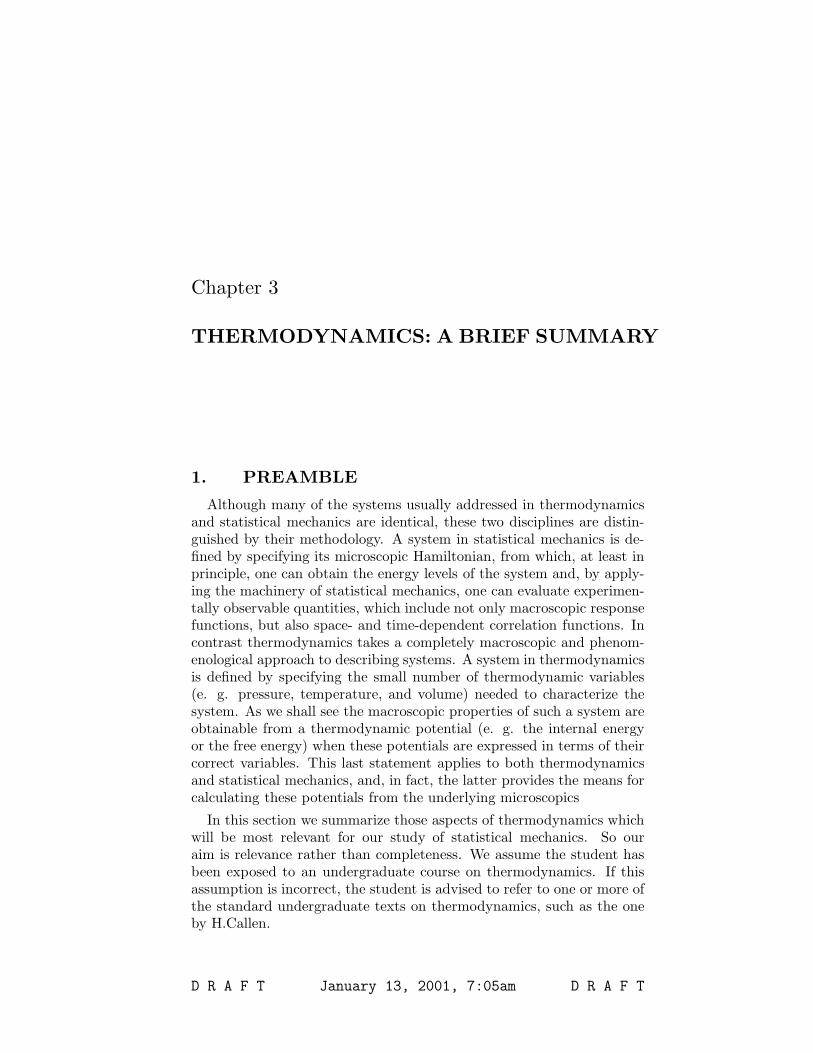
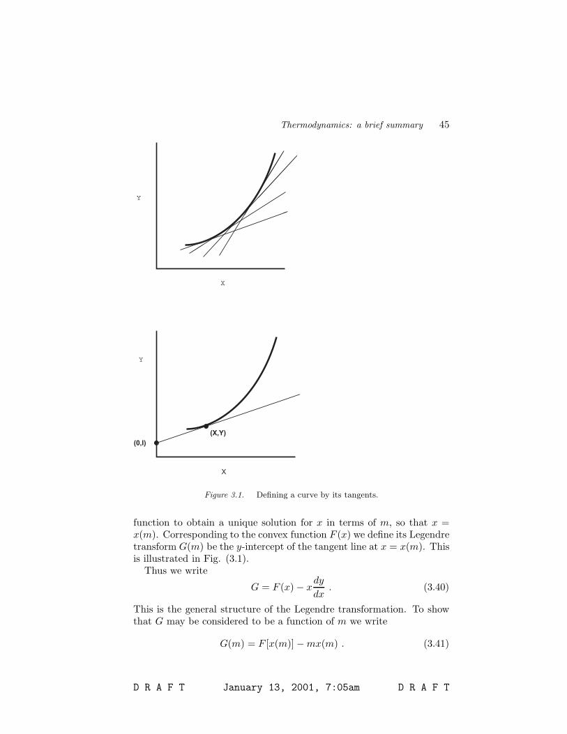
Say that you know some convex function, F (x). (“Convex” meansthat line segments connecting any two points, (x1, y(x1)) and (x2, y(x2),all lie on the same side of the curve. If the function is convex upwardsit always has a positive second derivative. If it is convex downwards itssecond derivative is always negative. In any event the second derivativecan not change sign as a function of x.) The stability relations for thethermodynamic potentials derived in Sec. 4.2 guarantee that they areconvex functions of their correct variables. (E. g. the internal energyU is a convex function of S and V .) Now consider the slope m ≡dF/dx as a function of x. Because F (x) is convex, we can invert this



Y

X

Y

X

(0,I)(X,Y)

Figure 3.1. Defining a curve by its tangents.

function to obtain a unique solution for x in terms of m, so that x =x(m). Corresponding to the convex function F (x) we define its Legendretransform G(m) be the y-intercept of the tangent line at x = x(m). Thisis illustrated in Fig. (3.1).

Thus we write

G = F (x) − xdy

dx. (3.40)

This is the general structure of the Legendre transformation. To showthat G may be considered to be a function of m we write

G(m) = F [x(m)] − mx(m) . (3.41)



We have thus constructed a unique function G(m) which is a functionof m = dy/dx. Furthermore, as we now show, the function G(m) con-tains all the information originally in F (x), because given G(m) we canwork backwards to construct F (x). To do this we construct, Φ(x), theLegendre transfomed function of G(m):

Φ(x) = G(m) −mdG

dm. (3.42)

¿From Eq. (3.41) we have

dG

dm=

dF

dx

dx

dm− m

dF

dmm − x

= −x . (3.43)

One can show that G is a convex function of M . Thus we can invert Eq.(3.42) to get x(m). Then Eq. (3.60) allows us to write

Φ = G(m) + mx , (3.44)

which we write as a function of x as

Φ(x) = G[m(x)] + m(x)x = F (x) . (3.45)

Thus we have reconstructed F (x) from G(m). It should be noted thatalthough we can reconstruct F (x) from a knowledge of G(m), we can notrecover that information if all we have is G(x). One can see this from Fig.(3.1): start by fixing one point on the curve F (x) versus x arbitrarily.Then knowing I(x) fixes the local slope which can be integrated to givethe full curve of F (x). But the fact that the intial point was arbitrarymeans that from G(x) we obtain a family of solutions for F (x). In otherwords, to perform the Legendre transformation we need the function interms of the correct variable. This is illustrated in the homework.

Applying this procedure to the dependence on S of U(S, V ), suggeststhat it is useful to define

F = U − ∂U

∂S

)V

S = U − TS . (3.46)

For fixed VdF = dU − TdS − SdT = −SdT . (3.47)

So F = F (T, V ), and S = −(∂F/∂T )T = S(T, V ). F is called theHelmholtz Free Energy. Its full differential is

dF = −SdT − pdV (3.48)



so that

S = −∂F

∂T

)V

, p = −∂F

∂V

)T

. (3.49)

We can also transform to the variables T and p ≡ ∂F/∂V )T by writing

G(T, p) = F − ∂F

∂V

)V

= F + pV (3.50)

dG = dF + pdV + V dp

= −SdT − pdV + pdV + V dp

= −SdT + V dp (3.51)

G is called the Gibbs Free Energy. It is a function only of thermody-namic fields (intensive variables).

One can also define the Enthalpy

H(S, p) = U − ∂U

∂V

)V

V = U + pV (3.52)

dH = TdS − pdV + pdV + V dp

= TdS + V dp (3.53)

which is useful, for example, for describing the cooling power of cryogenicliquids.

The extensive property or “additivity” of all of these thermodynamicpotential functions implies that they can each be written as n, the num-ber of moles, times a function of densities and fields that do not dependon n:

U(S, V ) = nu(S/n, V/n), (3.54)F (T, V ) = n f(T, V/n), (3.55)H(S, p) = nh(S/n, p), (3.56)G(T, p) = n g(T, p). (3.57)

It is important to realize that all the thermodynamic functions can beobtained from any one of these potentials providing the potential is givenin terms of the correct variables. For instance, for F the correct variablesare T and V , for G the correct variables are T and p, and so forth. Ahomework problem illustrates that a knowledge of a potential in terms ofincorrect variables does not determine all the thermodynamic functions.



For magnetic systems the same situations applies. Consider the mag-netic free energy, F , defined so that function F = U − TS, so that

dF = −SdT − M · dH .

This function will be minimized as a function of internal constraints forfixed temperature and applied field. Similar statements go through fora free energy which depends also on the volume:

dF = −SdT − M · dH − pdV .

(Strictly speaking, in the presence of a field the pressure is no longerisotropic and it is necessary to replace the pressure and volume by theappropriate stress and strain tensors. What this means is that if weapply a magnetic field along the z-axis to a cubical box of gas with sidesperpendicular to the Cartesian axes, the force the gas exerts on the facesperpendicular to the z-axis will be different from the force the gas exertson the other faces.)

6. APPLICATION TO PHASE TRANSITIONSWe start by reviewing the basic phenomenology of pure substances.

In the accompanying figure file we show a) isotherms for gases whichrange at high temperature from being very nearly ideal (pV = const)to the critical isotherm and then to isotherms which pass through thegas-liquid phase transition. In these diagrams the number n of moles(n = 1) is held fixed, so that in the single phase region the state of thegas is specified by fixing, for instance, the pressure and the temperature.Notice that the two phase region (which is indeed a region in the p-Vplane) is simply a line in the p-T plane. That means that in the twophase region p is a function of T : p = p(T ). In that case the completespecification can either be accomplished by giving V and T , or by givingT and the fraction xg of the system which is in the gas phase. Whenthe isotherm passes through the two phase region xg varies from 0 to 1as you increase the volume from that of the liquid to that of the gas.

To treat this two phase region thermodynamically, we study the equa-tion

dS =∂S

∂T

∣∣∣∣V

dT +∂S

∂V

∣∣∣∣T

dV .

Let the end points on an isotherm which passes through the two phaseregion be labeled A and B, with A referring to the liquid and B to thegas. Then we integrate Eq. (3.57) to get

SB − SA =∫ B

A

∂S

∂T

∣∣∣∣V

dT +∫ B

A

∂S

∂V

∣∣∣∣T

dV



=∫ B

A

∂S

∂V

∣∣∣∣T

dV . (3.58)

But recall

dF = −SdT − pdV ,

so that

∂S

∂V

∣∣∣∣T

=∂p

∂T

∣∣∣∣V

=dp

dT.

Thus Eq. (3.57) gives

SB − SA =dp

dT[VB − VA] ,

which is known as the Clausius-Clapeyron Equation. Note that theleft-hand side of this equation is related to the heat of vaporization,∆QAB = T (SB − SA). For liquid-gas or solid-gas transitions this equa-tion guarantees that dp/dT is positive. For solid-liquid transitions dp/dTis usually positive, but for water (which expands when it freezes) dp/dTis negative. The fact that water freezes from the top down is good formarine life.

7. THERMODYNAMICS OF OPEN SYSTEMSUp to now we have considered only systems with a fixed number

of particles, or more properly from a macroscopic point of view, a fixednumber of moles. Now let us broaden our field of view to include systemswhich consist of Ni particles of species ”i” for i = 1, 2, . . .. Then we write

dU = TdS − pdV +∑

i

µidNi ,

to express the fact that the internal energy can change because we addparticles to the system. From Eq. (3.58) we deduce that µi is the rate ofincrease in internal energy per added particle of species ”i”, AT FIXEDENTROPY AND VOLUME. Similarly the other potentials are definedby

dF = −SdT − pdV +∑

i

µidNi , (3.59)

dG = −SdT + V dp +∑

i

µidNi , (3.60)

dH = TdS + V dp +∑

i

µidNi . (3.61)



Thus Eq. (3.59) shows that µi is the rate of increase in the free energy,F , AT FIXED TEMPERATURE AND VOLUME per added particle ofspecies ”i”. Perhaps the most important of these is Eq. (3.60) whichsays that µi is the rate of increase in Gibbs free energy, G, AT FIXEDTEMPERATURE AND PRESSURE per added particle of species ”i”.

How could one experimentally attain an open system? One can imag-ine a solid or a liquid in contact with a gas of that material via a smallpipe. (What you want is to weakly couple your system to a particle reser-voir.) Alternatively, instead of a wall, have a membrane which allowsmolecules to pass from the reservoir to the system in question.

7.1 GIBBS-DUHEM RELATIONLook again at Eq. (3.60) and consider a process in which we simply

increase all the extensive variables (volume, mole numbers, thermody-namic potentials) by a scale factor, dλ. The result of this is clearly thatit will NOT cause the intensive variables T , p, µi to vary. It will causeG to change to G(1 + dλ), so that (with dT = dp = 0) we have

dG = Gdλ = −SdT = V dp +∑

i

µidNi =∑

i

µiNidλ , (3.62)

so that

G =∑

i

µiNi . (3.63)

Then dG =∑

i(µidNi + Nidµi) and we have the Gibbs-Duhem relation

0 = −SdT − V dp −∑

i

Nidµi .

For a system consisting of a single pure substance, Eq. (3.63) tells usthat µ is simply the Gibbs free energy per particle.

7.2 THE GRAND CANONICAL POTENTIALWe can also define a thermodynamic potential function for a systme

with a single species of particle Ω(T, V, µ), related to F (T, V,N) by aLegendre transformation and to G = F + pV by

Ω = F − µN = (G − pV ) − µN = −pV . (3.64)

where we used Eq. (3.63). Ω(T, V, µ) is called the Grand Canonicalpotential and, as we shall see, is often the most convenient potential tocalculate for quantum systems using statistical mechanics. This function



obeys

dΩ = dF − µdN − Ndµ − SdT − pdV µdN − µdN − Ndµ

= −SdT − pdV − Ndµ . (3.65)

Thus from a knowledge of Ω in terms of its appropriate we can get allthe thermodynamic functions via

S = −∂Ω∂T

)V,µ

(3.66)

p = −∂Ω∂V

)T,µ

(3.67)

N = −∂Ω∂µ

)V,T

. (3.68)

Usually one wants to get the thermodynamic functions as functions of Nrather than of µ. To do that one solves Eq. (3.68) for N in terms of µ, T ,and V . Then one uses Eqs. (3.66) and (3.67) to get the thermodynamicfunctions in terms of T , V , and µ(T, V,N). One can also use Eq. (3.64)to get the equation of state. But in this form the result will involve µrather than N .

7.3 PHASE EQUILIBRIUMSimilarly, we can apply these ideas to a system consisting of two phases

(e. g. liquid and gas) of a single substance in equilibrium. Then we write

G(T, p,Ni) = Nliqµliq(T, p) + Ngasµgas(T, p)= Nliqµliq(T, p) + [Ntot − Nliq]µgas(T, p) , (3.69)

where the susbscripts “tot,” “liq,” and “gas” indicate the total numberof particles, the number of particles in the liquid phase, and the numberof particles in the gas phase, respectively. Thus, as a function of nliq, Gcan be extremal only if

µliq(T, p) = µgas(T, p) . (3.70)

(In fact G is independent of the fraction of particles in each phase whenthis condition is fulfilled. Otherwise, when the condition is not fulfilledG is lower for one of the single phases than for phase coexistence.) Thismeans that although originally p and T could be considered to be in-dependent variables, the condition of phase equilibrium implies that the



chemical potentials in the two phases be equal. This implies a func-tional relation between p and T : as we said before at phase coexistencep = p(T ).

Obviously Eq. (3.70) has the very intuitive interpretation that as amolecule goes from one phase to the other, its chemical potential doesnot have to change. This is the microscopic interpretation of equilibrium.

Equation (3.70) is a simple example of the Gibbs ”phase rule,” whichis

f = c − φ + 2 ,

where f is the number of free variables (i. e. intensive variables) whichmay independently be fixed, c is the number of different substances,and φ is the number of phases (solid, liquid, gas, etc) present. For asingle substance we have seen that when φ = 2 only f = 1 intensivevariable can be fixed. When φ = 3 there are NO free variables. Thusthe triple point (where solid, liquid, and gas coexist) is an isolated pointin the phase diagram. For H2O the triple point occurs at T = 273.16 K(defined) and at p = 610 Pascals. (1 atm ≈ 105 Pascals.)

7.4 CHEMICAL POTENTIAL FOR A PURESYSTEM

Look again at Eq. (3.63) and consider what it says for a pure system.We know that G can be taken to be a function of n, T , and p and thatG is proportional to n. It thus implies that

µ = µ(T, p) . (3.71)

For an ideal gas you will show (in homework) that you can write

µ ≡ G/n = RT [φ(T ) + ln p] ,

where φ is a function only of T . From the form of φ(T ) one can seethat µ(n, T, V ) becomes negative are and large in magnitude when T →∞. Moreover, as the temperature is increased from zero the chemicalpotential initially has to decrease if the V and n are held fixed. To seethat note, from Eq. (3.62) that

∂µ

∂T

)p,N

= − S

N. (3.72)

Then

∂µ

∂T

)N,V

=∂µ

∂T

)N,p

+∂µ

∂p

)N,T

∂p

∂T

)N,V



= − S

N+

∂µ

∂p

)N,T

∂S

∂V

)N,T

→ − S

N≤ 0 . (3.73)

Thus, at low and high temperature thermodynamics requires µ(T, V,N)to decrease as T is increased.

8. EXERCISES (IN RANDOM ORDER)1. This problem illustrates the Legendre tranformaion and the notationis that of Sec. (5.). Take F (x) = ax2 + bx + c.

a) Is this function convex?b) Construct x(m).c) Construct G(m).d) Is G(m) convex?e) Using a knowledge of G(m) (and the fact that dG/dm = −x)

reconstruct F (x).f) Assume that dG/dm = −x and that you are given not G(m),

but rather G(x) ≡ G[x(m)], where G is the solution you found above..Display the family of functions F (x) which give rise to the given G(x).(In this special case, it is obvious from the fact that G(x) does not involveall the parameters a, b, and c that we can not completely specify F (x).)

2. Blackboard problems 2-6 of homework assignment #1.

3. Blackboard problem 1 of homework assignment #2.

4. This problem concerns equilibrium for a system contained in a boxwith fixed rigid walls, isolated from its surroundings, and consisting ofa gas with a partition separating the two subsystems of gas. Find theconditions for equilibrium from the maximum entropy principle when

a) the partition is fixed in position, does not allow transfer of particles,but does allow the transfer of energy.

b) the partition does not allow the transfer of particles, but does allowthe transfer of energy and the partition is movable.

andc) the partition is not movable, but does allow the transfer of particles

and the transfer of energy.

d) We believe that a partition which is movable but does not allowthe transfer of energy is unphysical. What would be the condition foreqiulibrium according to the principle of maximum entropy? (Assume,for simplicity that the partition does not allow the transfer of particles.)



5. From the thermodynamics review problems on blackboard the follow-ing problem (with minor editting) might be OK.1, 2, 5 (heavily editted), 7, 14, 17, 21, 22, 27, 29, 33.

6 I would like to see some problem that illustrates the behavior of thechemical potential as a function of temperature.


Documents

Chapter 3 THERMODYNAMICS: A BRIEF SUMMARYharris/thermo.pdf · Chapter 3 THERMODYNAMICS: A BRIEF SUMMARY 1. PREAMBLE Although many of the systems usually addressed in thermodynamics