19

CHAPTER 3THE COMMON FACTOR MODEL IN THE POPULATION

FromExploratory Factor Analysis

Ledyard R Tuckerand

Robert C. MacCallum

©1997

20

CHAPTER 3

THE COMMON FACTOR MODEL IN THE POPULATION

3.0. Introduction

In Chapter 1 we presented a conceptual, non-mathematical view of common factor

theory. The purpose of the present chapter is to develop a detailed mathematical framework for

this approach. Such a framework will serve the dual purpose of (a) providing an explicit

representation of common factor theory as a mathematical model, so that its properties and

implications can be understood; and (b) providing a basis for the solution of the problem, to be

addressed in Chapter 7, of fitting the model to observed data.

The common factor model will be developed in this chapter in the context of a

population. That is, we will express the model in terms of population parameters rather than

sample statistics. Issues of sampling and parameter estimation will be treated in later chapters.

So, for now, the reader should conceive of the case where the theoretical population of

observations is available. The development of the model and the discussion of related topics and

issues will require the use of rather extensive mathematical notation. In general, we will adhere

to a notational system where population parameters are represented by Greek letters and

italicized English letters. Sample statistics (though none are used in this chapter) will be

presented by normal (un-italicized) English letters. A glossary of notation is presented for the

reader's use in Appendix A. The approach taken in this mathematical presentation employs linear

algebra, or matrix algebra. Readers must be comfortable with matrix terminology and

manipulations in order to follow easily the developments to be presented. A basic review of

matrix operations is presented in Appendix B. In addition, we will make use of a number of

operations and basic theorems involving linear transformations of attributes. These operations

and theorems are reviewed in Appendix C.

3.1. Algebraic Representation of the Common Factor Model

To begin, let us recall the basic concepts of common factor theory as presented in

Chapter 1. For a given battery of surface attributes, there will exist a set of factors. These factors

will be of three different types of common, specific, and error of measurement. The common

factors are those that affect more than one attribute in the set, and specific and error of

measurement factors each affect a single attribute. Each surface attribute is, to a degree, linearly

dependent on these underlying factors. The variation in a surface attribute is accounted for in part

by its dependence on common, specific, and error of measurement factors. The covariation

between any two surface attributes is accounted for in part by their joint dependence on one or

more of the same common factors. Since common factor theory cannot be expected to represent

21

the real world precisely, it is not expected that the variation and covariation of the surface

attributes will be exactly explained by the underlying common, specific, and error of

measurement factors.

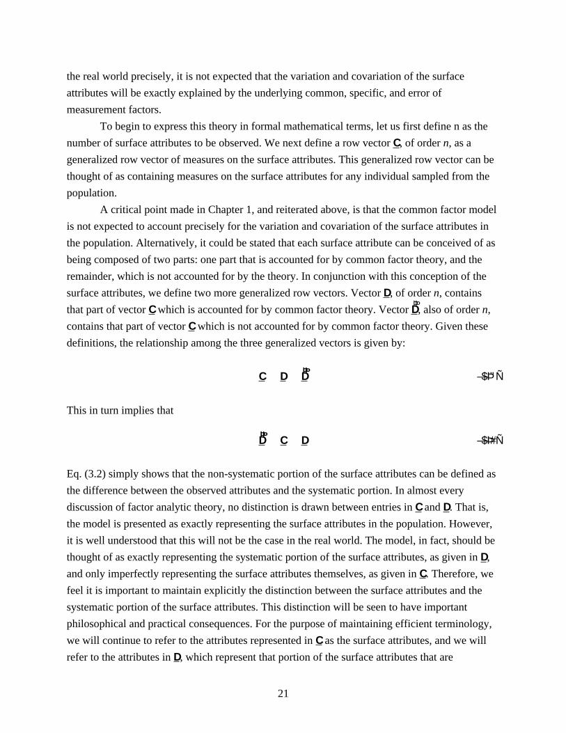
To begin to express this theory in formal mathematical terms, let us first define n as the

number of surface attributes to be observed. We next define a row vector , of order , as aC n

generalized row vector of measures on the surface attributes. This generalized row vector can be

thought of as containing measures on the surface attributes for any individual sampled from the

population.

A critical point made in Chapter 1, and reiterated above, is that the common factor model

is not expected to account precisely for the variation and covariation of the surface attributes in

the population. Alternatively, it could be stated that each surface attribute can be conceived of as

being composed of two parts: one part that is accounted for by common factor theory, and the

remainder, which is not accounted for by the theory. In conjunction with this conception of the

surface attributes, we define two more generalized row vectors. Vector , of order , containsD n

that part of vector which is accounted for by common factor theory. Vector , also of order ,C DÞÞ

n

contains that part of vector which is not accounted for by common factor theory. Given theseC

definitions, the relationship among the three generalized vectors is given by:

C D Dú ÄÞÞ

Ð$Þ"Ñ

This in turn implies that

D C DÞÞ

ú Å Ð$Þ#Ñ

Eq. (3.2) simply shows that the non-systematic portion of the surface attributes can be defined as

the difference between the observed attributes and the systematic portion. In almost every

discussion of factor analytic theory, no distinction is drawn between entries in and . That is,C D

the model is presented as exactly representing the surface attributes in the population. However,

it is well understood that this will not be the case in the real world. The model, in fact, should be

thought of as exactly representing the systematic portion of the surface attributes, as given in ,D

and only imperfectly representing the surface attributes themselves, as given in . Therefore, weC

feel it is important to maintain explicitly the distinction between the surface attributes and the

systematic portion of the surface attributes. This distinction will be seen to have important

philosophical and practical consequences. For the purpose of maintaining efficient terminology,

we will continue to refer to the attributes represented in as the surface attributes, and we willC

refer to the attributes in , which represent that portion of the surface attributes that areD

22

accounted for by the common factor model, as . In addition, we will refer tomodeled attributes

entries in as ; again, these values represent that portion of the surface attributes notDÞÞ

errors of fit

accounted for by the model.

As discussed earlier, factor analytic theory postulates the existence of underlying internal

attributes, or factors. Let represent a generalized row vector of measures on the factors. TheB

vector will be of order , where is the total number of factors of all three types. Thus, thisB m m

vector contains the (unobservable) measures for an individual on the common, specific, and error

of measurement factors. Next, let us define a matrix containing weights which represent theH

effects of the factors on the modeled attribute. This matrix will be of order , where then mÇ

rows represent the modeled attributes and the columns represent the factors. An entry is a=45

weight, analogous to a regression weight, representing the effects of factor on modeled attributek

j. Given these definitions, the common factor model can be represented simply as

D Bú Hw Ð$Þ$Ñ

This equation simply defines each modeled attribute as a linear combination of the measures on

the factors. This representation of the model can be stated in an expanded fashion by

incorporating the distinction among common, specific and error of measurement factors. The

vector containing measures on the factors can be conceived of as containing measures on theB

types of factors. Let be the number of common factors, and recall that should be much lessr r

than , the number of attributes. We then can define as a row vector of order containingn rB"

measures on the common factors. In similar fashion, let contain measures on the specificB0

factors and let contain measures on the error of measurement factors. Both and will beB B B& 0 &

of order , since there is one specific factor and one error of measurement factor for eachn

attribute. For the present, the measures on all three types of factors will be defined as being given

in standardized form. As a result of the way in which the three types of factors have been

defined, the measures on the factors can be seen to have some interesting properties. In

particular, since the specific factors represent systematic portions of each modeled attribute

which are unique to each attribute, the specific factors must be uncorrelated with each other.

Similarly, since the error of measurement factors represent transient aspects of each modeled

attribute, they also must be uncorrelated with each other. Finally, the definitions of these two

types of factors also require that they be uncorrelated with each other and with the common

factors. The vectors of measures on the three types of factors can be adjoined horizontally to

form the super-vector , as followsB À

B B B Bú Ò ß ß Ó" 0 & Ð$Þ%Ñ

The order of , defined as above, now can be seen more clearly. The vector will containB Bm

23

measures on the common factors, the specific factors, and the error of measurement factors.r n n

Thus, the total number of factors, , is given bym

7 ú < Ä #8 Ð$Þ&Ñ

Just as the vector of measures on the factors can be seen as containing separate sections

corresponding to the three types of factors, so also can the factor weight matrix be partitioned.H

We can define weight matrices for each of the three types of factors. Let be a matrix of orderF

n r , where the rows represent the modeled attributes, the columns represent the commonÇ

factors, and each entry represents the weight for common factor on modeled attribute . Let"45 k 4

B be a matrix of order , where the rows represent the modeled attributes, the columnsn nÇ

represent the specific factors, and each diagonal entry represents the weight for specific factor 04 j

on modeled attribute . Note that matrix will be diagonal, since each specific factor affects onlyj B

one modeled attribute. Similarly, let be an matrix, with rows representing modeledI n nÇ

attributes, columns representing error of measurement factors, and diagonal entries %4

representing the weight for error of measurement factor on modeled attribute . This matrix ofj j

error of measurement factor weights must also be diagonal, since each error of measurement

factor affects only one modeled attribute. These three matrices of factor weights then can be

adjoined horizontally to form the full matrix actor weights:H of f

H Bú ÒFß ß IÓ Ð$Þ'Ñ

Thus, can be seen to be a super-matrix containing the three separate matrices of factor weightsH

representing the three types of factors.

The representations of and given in Eqs. (3.4) and (3.6) respectively can beB H

substituted into Eq. (3.3) to provide an expanded representation of the common factor model, as

follows:

D B B B B B Bú Ò ß ß Ó F IF

I" 0 & " 0 &

Ô ×Õ Ø

w

w

w

w w wB Bú Ä Ä Ð$Þ(Ñ

This representation of the model shows more clearly that each modeled attribute is defined as a

linear combination of the common, specific, and error of measurement factors. Furthermore,

given that and are diagonal, it can be seen that each modeled attribute is represented as aB I

linear combination of common factors, one specific factor, and one error of measurementr

factor.

An interesting aspect of this representation is that error of measurement factors contribute

to the modeled attributes. Recognition of this fact should help the reader distinguish between

errors of measurement, which give rise to error of measurement factors, and errors of fit, which

24

were defined in Eq. (3.2). Errors of measurement are represented explicitly in the model and

contribute to the modeled attributes. Errors of fit represent the lack of fit of the model to the real

world, or the lack of correspondence between the modeled attributes and the surface attributes.

As defined to this point, the common factor model represents the underlying structure of

each modeled attribute. Recall from Chapter 1 that the general objective of factor analysis is to

account for the variation and covariation of the attributes. To achieve this, it is necessary to

express the model in terms of the variances and covariances of the modeled attributes. This can

be accomplished fairly easily by making use of theorems presented in Appendix C. We are

dealing with a situation where we have two sets of attributes (the modeled attributes and the

factors) which are related via a linear transformation as defined in Eq. (3.3). In this case it is

possible to define a functional relationship between the covariances of the two sets of attributes,

as shown in Appendix C. Let us define as a population covariance matrix for the modeledDDD

attributes. The matrix will be of order , with diagonal entries representing theDDD n nÇ 544

population variance of modeled attribute , and off-diagonal entries representing thej 524

population covariance of modeled attributes and . Let us next define as a populationh j DBB

covariance matrix for the factors. Matrix will be of order and will contain entriesDBB m mÇ

556 representing the population variances (on the diagonal) and covariances (off the diagonal) of

the factors. The relationship between and can be obtained by direct application ofD DDD BB

Corollary 3 of Theorem 4 in Appendix C. This yields

D H D HDD BBwú Ð$Þ)Ñ

This equation represents the common factor model in terms of covariances of modeled attributes

and factors. It states that the variances and covariances of the modeled attributes are a function of

the factor weights and the variance and covariances of the factors.

It is informative to consider a more detailed version of Eq. (3.8), which can be obtained

by incorporating the distinction among common, specific, and error of measurement factors.

First, let us consider more closely the nature of . It will be shown that this matrix has a veryDBB

simple and interesting form. Recall that we are defining the measures on the to be infactors

standardized form. Therefore, the matrix will take the form of a correlation matrix. RecallDBB

also that there exist three different types of factors (common, specific, and error of

measurement), as defined in Eq. (3.6). This implies that can be thought of as a super-DBB

matrix, with sub-matrices containing correlations within or between types of factors as follows:

D

D D DD D DD D D

BB úÔ ×Õ Ø

"" "0 "&

0" 00 0&

&" &0 &&

Ð$Þ*Ñ

25

For each sub-matrix in , the first subscript represents the factors defined by the rows of theDBB

sub-matrix, and the second subscript represents the factors defined by the columns of the

sub-matrix. For example, the sub-matrix will be of order and will containD0" n rÇ

correlations between specific factors (rows) and common factors (columns). Given this

representation of , it is very useful to consider the nature of the sub-matrices. ConsideringDBB

the diagonal submatrices in Eq. (3.9), note that these contain correlations among the factors

within each given type (common, specific, error of measurement). Since the common factors may

be correlated with each other, let us define

F ú $Þ"!ÑD"" (

Matrix will be of order and will contain intercorrelations among the common factors. ItF r rÇ

was noted earlier that specific factors will be mutually uncorrelated, as will error of measurement

factors. Therefore, it can be stated that

D00 ú M Ð$Þ""Ñ

and

D%% ú M Ð$Þ"#Ñ

The identity matrices shown in Eqs. (3.11) and (3.12) will be of order . Considering then

off-diagonal sections of shown in Eq. (3.9), it can be seen that these submatrices willDBB

contain all zeroes. Each of these sub-matrices represents a matrix of intercorrelations among

factors of two different types (common and specific, common and error of measurement, specific

and error of measurement), and, as was explained earlier in this section, factors of different types

are, by definition, uncorrelated in the population. Given these properties of the sub-matrices in

Eq. (3.9), we can rewrite that equation as

DF

BB ú $Þ"$Ô ×Õ Ø

! !! M !! ! M

( )

A very important representation of the common factor model can now be obtained by substitution

of the super-matrix form of , from Eq. (3.6), and , from Eq. (3.13), into the model asH DBB

shown in Eq. (3.8). This yields

D BF

BDD

w

w

wú ÒFß ß I Ó

! ! F! M !! ! M I

Ô ×Ô ×Õ ØÕ Ø Ð$Þ"%Ñ

26

ú Ä ÄF F IF Bw # # Ð$Þ"&Ñ

This equation shows that the population covariances for the modeled attributes are functions of

the weights and intercorrelatlons for the common factors, the squared specific factor weights, and

the squared error of measurement factor weights. When the common factor model is written in

this form, the mathematical representation of the model can be seen to be consistent with the

basic principles of common factor theory discussed in Chapter 1. In particular, it was stated that

the common factors alone account for the relationships among the modeled attributes. This is

revealed in Eq. (3.15) by the fact that the off-diagonal elements of are a function of only theDDD

parameters in the term . Thus, the common factor weights and intercorrelations combineF FF '

to account for the relationships among the modeled attributes. Another principle of common

factor theory is that the variation in the modeled attributes is explained by all three types of

factors. In mathematical terms, this is seen in Eq. (3.15) in that the diagonal elements of areDDD

a function of the common factor parameters in , as well as the diagonal elements in F FF ' B#

and . Thus, since and are diagonal, the specific and error of measurement factors canI I# # #B

be seen as contributing only to the variances of the modeled attributes (i.e., the diagonal elements

of , and not the covariances.DDDÑ

This view implies that it should be possible to define separate components of the variance

of each modeled attribute; i.e., portions due to common, specific, and error of measurement

factors. This is, in fact, quite simple and will be seen to provide useful information. Let us define

a diagonal matrix asL#

L H3+1ÐF F Ñ# wú F Ð$Þ"'Ñ

Matrix will be diagonal and of order , with diagonal elements representing theH# n n hÇ 4#

amount of variance in modeled attribute that is accounted for by the common factors. This willj

be referred to as the common variance of modeled attribute . It can be seen thatj

H3+1Ð Ñ L ID BDD# # #ú Ä Ä Ð$Þ"(Ñ

In terms of the variance of a given modeled attribute , this implies thatj

5 0 %44 4 4 4# #ú Ä Ä2 # Ð$Þ")Ñ

Thus, the variance of each modeled attribute is made up of a common portion, a specific portion,

and an error of measurement portion. It is interesting to convert these variance components into

proportions by dividing each side of Eq. (3.18) by This yields544Þ

5 5 5 0 544 44 44 444 4# #Î ú 2 Î Ä Î Ä Ð$Þ"*Ñ% 54

#44Î ú "

27

If we define

2 2 ε

4 4# #

44ú 5 Ð$Þ#!Ñ

0#4

µÎú 0 54

#44 Ð$Þ#"Ñ

% % 54 4# #

44

µÎú Ð$Þ##Ñ

we then can note that for any modeled attribute, we obtain

2 "µ µ µ

4 4 4# # #Ä Ä ú0 % Ð$Þ##Ñ

These three proportions of variance are important characteristics of the modeled attributes. The

first, represents the proportion of variance in modeled attribute that is due to the common2 ßµ

4# j

factors. This quantity is called the of modeled attribute . The second, communality j 04#

µß

represents the proportion of variance in modeled attribute that is due to the specific factor forj

that attribute. This quantity is called the for modeled attribute . The third, specificity j %#4

µß

represents the proportion of variance in modeled attribute that is due to the error factor for thatj

attribute This quantity is called the for modeled attribute . Noteerror of measurement variance j

that we can define diagonal matrices , containing these proportions of varianceL Iµ µ µ

# # #, , and B

for the modeled attributes. Let us define a diagonal matrix containing the variances ofn Ò ÓD. DD

the modeled attributes. That is,

Ò Ó H3+1 Ð ÑD D. DD DDú Ð$Þ#%Ñ

Following Eqs. (3.20)-(3.22), we then can define matrices L Iµ µ µ

# # #, , and as follows:B

L L Ò Óµ

# #. DDú Ð$Þ#&ÑD

Å"

B B D# #. DD

µÒ Óú Ð$Þ#'Ñ

Å"

I I Ò Óµ

# #. DDú Ð$Þ#(ÑD

Å"

According to Eq. (3.23), the sum of these matrices would be an identity matrix:

L I Mµ µ µ

# # #Ä Ä úB Ð$Þ#)Ñ

28

There are two interesting variance coefficients which can be derived from the three types

of variance defined in the common factor model. The first is the of a modeled attribute.reliability

Reliability is defined in mental test theory as unity minus the error of measurement variance for

standardized measures. In the present context, this can be written

< ú " Å Ð$Þ#*Ñ4 %4#

µ

where is the reliability of modeled attribute . Based on Eq. (3.23), we can rewrite Eq. (3.29)r j4

as

< ú Ð$Þ$!Ñ4 2 ĵ µ

4 4# #0

This equation implies that, in factor analytic terms, reliability is the sum of the variances due to

the common factors and the specific factor, or, in other words, the sum of the communality and

specificity. Since reliability is defined as true score variance, this result means that true score

variance can be represented as the sum of the two types of systematic variance in the common

factor model: that due to the common factors and that due to the specific factor.

An alternative combination of components of variance is to sum the specific and error

portions for each modeled attribute. This sum would yield a portion which is called unique

variance; i.e., that due to factors (both systematic and error of measurement) which affect only

one attribute. In unstandardized form this would be written

Y I# # #ú ÄB Ð$Þ$"Ñ

where is a diagonal matrix with entries representing the variance in modeled attribute Y # ?#4 j

due to specific and error of measurement factors. In terms of the variance expressed as

proportions, we would write

Y Iµ µ µ

# # #ú ÄB Ð$Þ$ Ñ2

where is a diagonal matrix with entries representing the of variance inYµ

# ?µ

#4 proportion

modeled attribute due to specific and error of measurement factors. This proportion is called thej

uniqueness of modeled attribute , and is defined as the sum of the specificity and error ofj

measurement variance of that attribute. The relation between the uniquenesses of the modeled

attributes, defined in Eq. (3.32), and the unique variances, defined in Eq. (3.31), can be obtained

by substitution from Eqs. (3.26) and (3.27) into Eq. (3.32). This yields the following:

Y Y Ò Óµ

# #. DDú D

Å"

Ð$Þ$$Ñ

29

This relation follows those given in Eqs. (3.25)-(3.27) for other variance components and merely

represents the conversion of unique variances into proportions called uniqueness. A final

interesting relation is obtained by substituting from Eq. (3.32) into Eq. (3.28), yielding

L Y Mµ µ

# #Ä ú Ð$Þ$%Ñ

This equation simply implies that the communality plus the uniqueness for each modeled

attribute will equal unity. In other words, the variance of a modeled attribute can be viewed as

arising from two sources: (a) the common factors, or influences which are common to other

attributes in the battery; and (b) the unique factors, or influences which are unique to the given

attribute.

A most important equation is produced by substituting from Eq. (3.31) into the

expression for the common factor model given in Eq. (3. 15). This yields

D FDDw #ú ÄF F Y Ð$Þ$&Ñ

Alternatively, we could write

D FDD# wÅ úY F F Ð$Þ$'Ñ

In either form, these equations provide a very fundamental expression of the common factor

model. They show the functional relationship between the population variances and covariances

of the modeled attributes, given in , and critical parameters of the model contained in , theDDD F

matrix of common factor weights, , the matrix of common factor intercorrelations, and , theF Y #

diagonal matrix of unique variances. As will be seen in subsequent chapters, this expression of

the model provides a basis for some procedures for estimating model parameters. Thus, Eq.

(3.35) should be viewed as a fundamental equation of common factor theory, expressing the

common factor model in terms of the variance and covariances of the modeled attributes. It is

important to understand, however, that this version of the model is a derived statement, i.e.,

derived from the model as given in Eq. (3.3), which defined the structure of the modeled

attributes themselves. That is, based on the model defined in Eq. (3.3), the model in Eq. (3.35),

defining the structure of the covariances of the modeled attributes as a function of correlated

common factors, is derived. Correlated common factors are also called common factors,oblique

and the model represented by Eq. (3.35) is called the .oblique common factor model

It is interesting and useful to recognize that the model given by Eq. (3.35) could have

been derived based on definitions of and slightly different than those given in Eqs. (3.4) andB H

(3.6), respectively. This alternative approach involves combining the specific and error of

measurement factor portions of the model into a unique factor portion at the outset. That is,

rather than define as containing scores on common, specific, and error of measurement factors,B

30

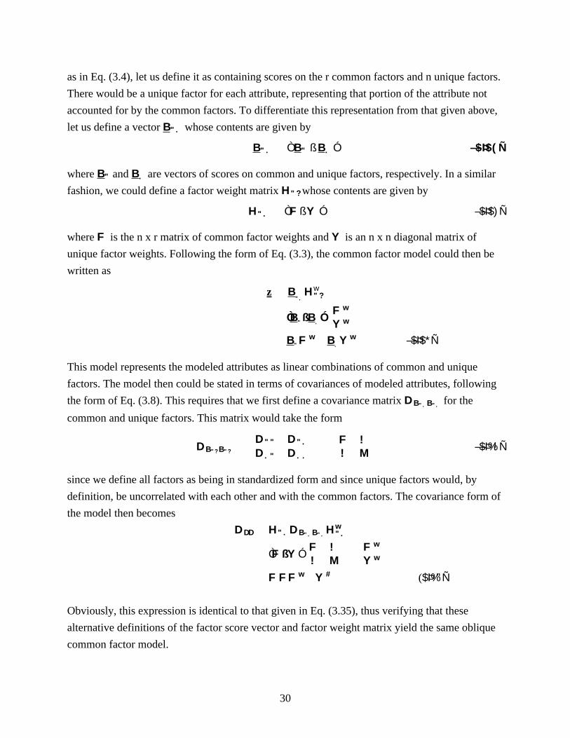
as in Eq. (3.4), let us define it as containing scores on the r common factors and n unique factors.

There would be a unique factor for each attribute, representing that portion of the attribute not

accounted for by the common factors. To differentiate this representation from that given above,

let us define a vector contents are given byB". whose

B B B". " .ú Ò ß Ó Ð$Þ$(Ñ

where and are vectors of scores on common and unique factors, respectively. In a similar B B" .

fashion, we could define a factor weight matrix hose contents are given byH"?w

H". ú Ò ß ÓF Y Ð$Þ$)Ñ

where is the n x r matrix of common factor weights and is an n x n diagonal matrix ofF Y

unique factor weights. Following the form of Eq. (3.3), the common factor model could then be

written as

z ú

ß ÓFY

F Ä Y

B

B B

B B

".

" .

" .

H"?

w

w

w w

w

ú

ú

Ò î ïÐ$Þ$*Ñ

This model represents the modeled attributes as linear combinations of common and unique

factors. The model then could be stated in terms of covariances of modeled attributes, following

the form of Eq. (3.8). This requires that we first define a covariance matrix DB B". ". for the

common and unique factors. This matrix would take the form

DD DD D

FB B" "? ?

ú úî ï î ï"" ".

." ..

!! M

Ð$Þ%!Ñ

since we define all factors as being in standardized form and since unique factors would, by

definition, be uncorrelated with each other and with the common factors. The covariance form of

the model then becomes

D H D HDD B Bwú ". ".". ".

ú Ò Ó

ú Ä $Þ%"Ñ

Fß Y! F

! M Y

F F Y

î ïî ïF

F

w

w

w # (

Obviously, this expression is identical to that given in Eq. (3.35), thus verifying that these

alternative definitions of the factor score vector and factor weight matrix yield the same oblique

common factor model.

31

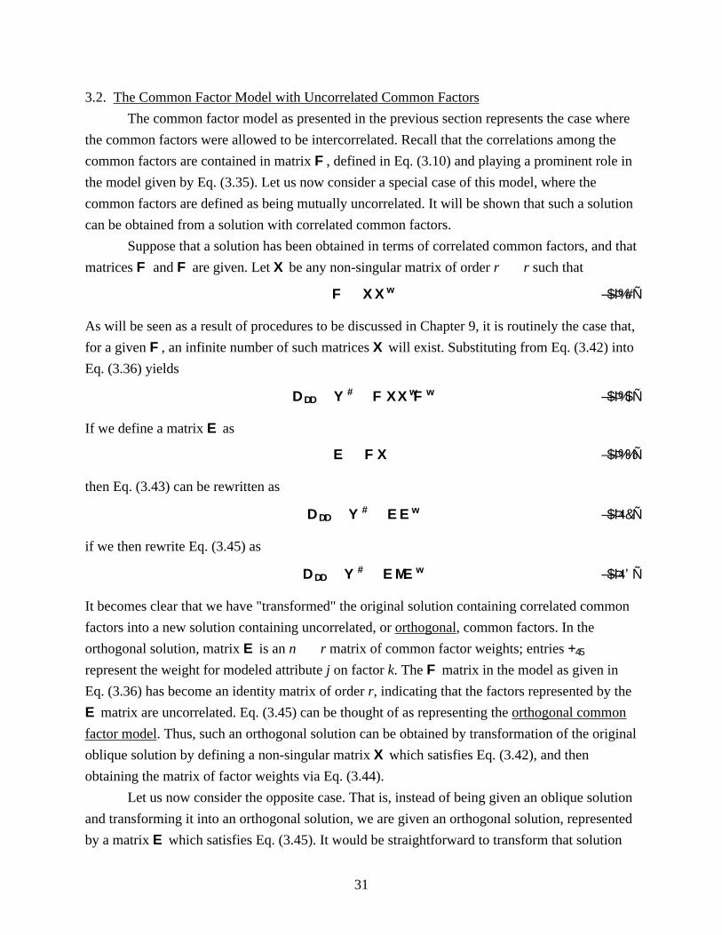
3.2. The Common Factor Model with Uncorrelated Common Factors

The common factor model as presented in the previous section represents the case where

the common factors were allowed to be intercorrelated. Recall that the correlations among the

common factors are contained in matrix , defined in Eq. (3.10) and playing a prominent role inF

the model given by Eq. (3.35). Let us now consider a special case of this model, where the

common factors are defined as being mutually uncorrelated. It will be shown that such a solution

can be obtained from a solution with correlated common factors.

Suppose that a solution has been obtained in terms of correlated common factors, and that

matrices and are given. Let be any non-singular matrix of order such thatF XF r rÇ

F ú Ð$Þ%#ÑX X w

As will be seen as a result of procedures to be discussed in Chapter 9, it is routinely the case that,

for a given , an infinite number of such matrices will exist. Substituting from Eq. (3.42) intoF X

Eq. (3.36) yields

DDD# w wÅ úY FXX F Ð$Þ%$Ñ

If we define a matrix asE

E FXú Ð$Þ%%Ñ

then Eq. (3.43) can be rewritten as

DDD# wÅ úY EE Ð$Þ &Ñ4

if we then rewrite Eq. (3.45) as

DDD# wÅ úY EME Ð$Þ 'Ñ4

It becomes clear that we have "transformed" the original solution containing correlated common

factors into a new solution containing uncorrelated, or , common factors. In theorthogonal

orthogonal solution, matrix is an matrix of common factor weights; entries E n rÇ +45

represent the weight for modeled attribute on factor . The matrix in the model as given inj k F

Eq. (3.36) has become an identity matrix of order , indicating that the factors represented by ther

E matrix are uncorrelated. Eq. (3.45) can be thought of as representing the orthogonal common

factor model. Thus, such an orthogonal solution can be obtained by transformation of the original

oblique solution by defining a non-singular matrix which satisfies Eq. (3.42), and thenX

obtaining the matrix of factor weights via Eq. (3.44).

Let us now consider the opposite case. That is, instead of being given an oblique solution

and transforming it into an orthogonal solution, we are given an orthogonal solution, represented

by a matrix which satisfies Eq. (3.45). It would be straightforward to transform that solutionE

32

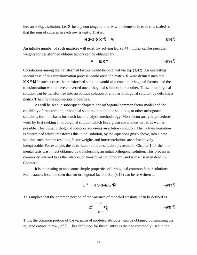
into an oblique solution. Let be any non-singular matrix with elements in each row scaled soX

that the sum of squares in each row is unity. That is,

H3+1ÐX X Ñ Mw ú Ð$Þ% Ñ7

An infinite number of such matrices will exist. By solving Eq. (3.44), it then can be seen that

weights for transformed oblique factors can be obtained by

F EXú Ð$Þ% Ñw 8

Correlations among the transformed factors would be obtained via Eq. (3,42). An interesting

special case of this transformation process would arise if a matrix were defined such thatX

X X w= . In such a case, the transformed solution would also contain orthogonal factors, and theM

transformation would have converted one orthogonal solution into another. Thus, an orthogonal

solution can be transformed into an oblique solution or another orthogonal solution by defining a

matrix having the appropriate properties.T

As will be seen in subsequent chapters, the orthogonal common factor model and the

capability of transforming orthogonal solution into oblique solutions, or other orthogonal

solutions, form the basis for much factor analysis methodology. Most factor analytic procedures

work by first seeking an orthogonal solution which fits a given covariance matrix as well as

possible. This initial orthogonal solution represents an arbitrary solution. Then a transformation

is determined which transforms this initial solution, by the equations given above, into a new

solution such that the resulting factor weights and intercorrelations are substantively

interpretable. For example, the three-factor oblique solution presented in Chapter 1 for the nine

mental tests was in fact obtained by transforming an initial orthogonal solution. This process is

commonly referred to as the rotation, or transformation problem, and is discussed in depth in

Chapter 9.

It is interesting to note some simple properties of orthogonal common factor solutions.

For instance, it can be seen that for orthogonal factors, Eq. (3.16) can be re-written as

L H3+1ÐEE Ñ# wú Ð$Þ%*Ñ

This implies that the common portion of the variance of modeled attribute can be defined asj

2 ú +# #4 40

0ú"

<" Ð$Þ&!Ñ

Thus, the common portion of the variance of modeled attribute j can be obtained by summing the

squared entries in row of . This definition for this quantity is the one commonly used in thej E

33

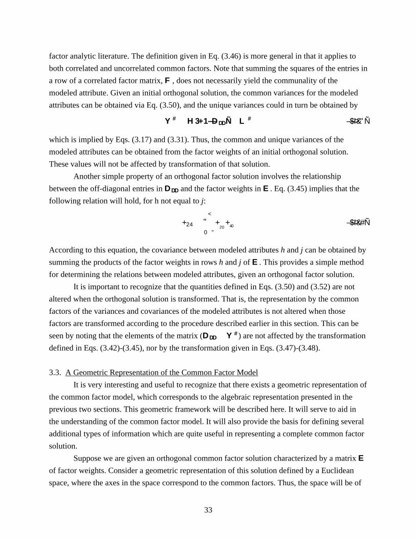
factor analytic literature. The definition given in Eq. (3.46) is more general in that it applies to

both correlated and uncorrelated common factors. Note that summing the squares of the entries in

a row of a correlated factor matrix, , does not necessarily yield the communality of theF

modeled attribute. Given an initial orthogonal solution, the common variances for the modeled

attributes can be obtained via Eq. (3.50), and the unique variances could in turn be obtained by

Y H3+1Ð Ñ L# #DDú ÅD Ð$Þ&"Ñ

which is implied by Eqs. (3.17) and (3.31). Thus, the common and unique variances of the

modeled attributes can be obtained from the factor weights of an initial orthogonal solution.

These values will not be affected by transformation of that solution.

Another simple property of an orthogonal factor solution involves the relationship

between the off-diagonal entries in and the factor weights in . Eq. (3.45) implies that theDDD E

following relation will hold, for h not equal to :j

+ ú + + Ð$Þ&#Ñ24

0ú"

<"20 40

According to this equation, the covariance between modeled attributes and can be obtained byh j

summing the products of the factor weights in rows and of . This provides a simple methodh j E

for determining the relations between modeled attributes, given an orthogonal factor solution.

It is important to recognize that the quantities defined in Eqs. (3.50) and (3.52) are not

altered when the orthogonal solution is transformed. That is, the representation by the common

factors of the variances and covariances of the modeled attributes is not altered when those

factors are transformed according to the procedure described earlier in this section. This can be

seen by noting that the elements of the matrix ( are not affected by the transformationDDD#Å Y )

defined in Eqs. (3.42)-(3.45), nor by the transformation given in Eqs. (3.47)-(3.48).

3.3. A Geometric Representation of the Common Factor Model

It is very interesting and useful to recognize that there exists a geometric representation of

the common factor model, which corresponds to the algebraic representation presented in the

previous two sections. This geometric framework will be described here. It will serve to aid in

the understanding of the common factor model. It will also provide the basis for defining several

additional types of information which are quite useful in representing a complete common factor

solution.

Suppose we are given an orthogonal common factor solution characterized by a matrix E

of factor weights. Consider a geometric representation of this solution defined by a Euclidean

space, where the axes in the space correspond to the common factors. Thus, the space will be of

34

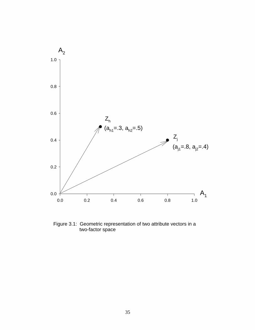
dimensionality . Let each modeled attribute be represented by a vector in the space, with ther

coordinates of the end-points of each factor weights for the corresponding modeled attribute.

Thus, there will be n vectors in the space. Figure 3.1 provides an illustration of such a space for a

case of two factors, designated A and A , and two modeled attributes, designated and The1 2 h jD D Þ

reader should keep in mind that this illustration is over-simplified in the sense that real world

cases would involve more attributes (vectors), and very often more factors (dimensions).

Nevertheless, this illustration will serve to demonstrate a number of important points. Note that

the axes are orthogonal, meaning that the common factors are uncorrelated. The coordinates of

the end-points of the two attribute vectors represent the factor weights for those attributes. These

values would correspond to the entries in rows and of the factor weight matrix . Such ah j E

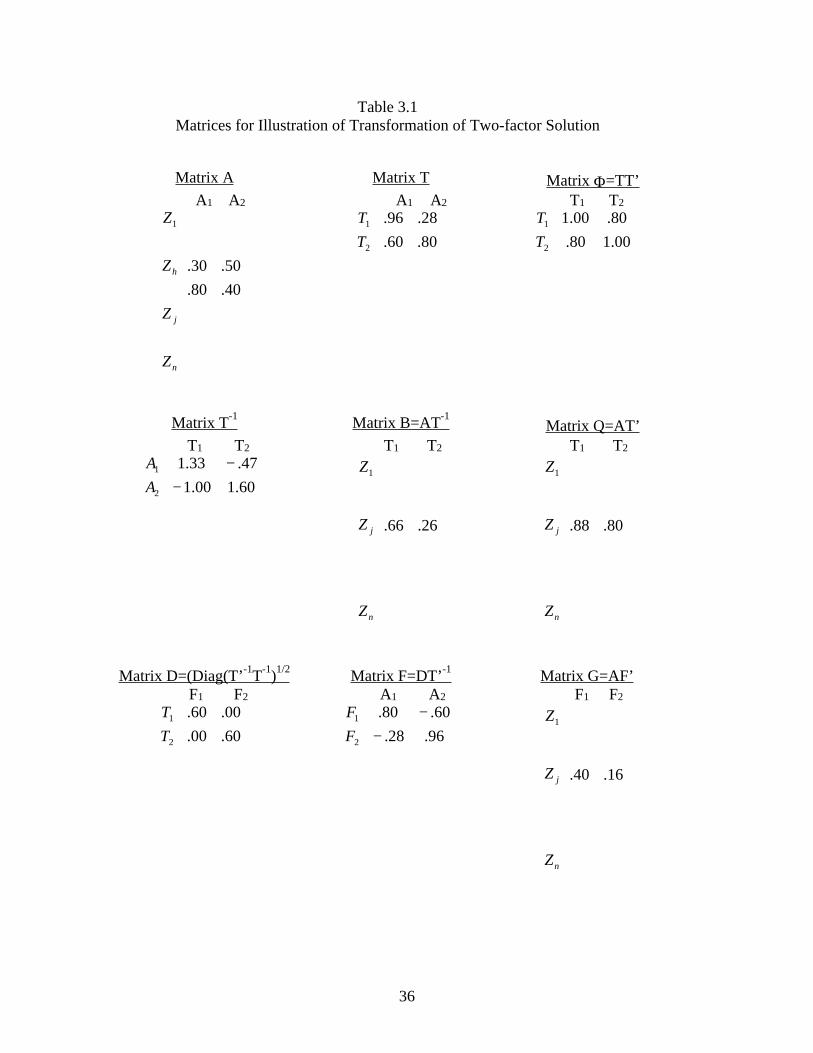
matrix, along with other information referred to below, is shown in Table 3.1.

It is interesting to consider some simple geometric properties of these modeled attribute

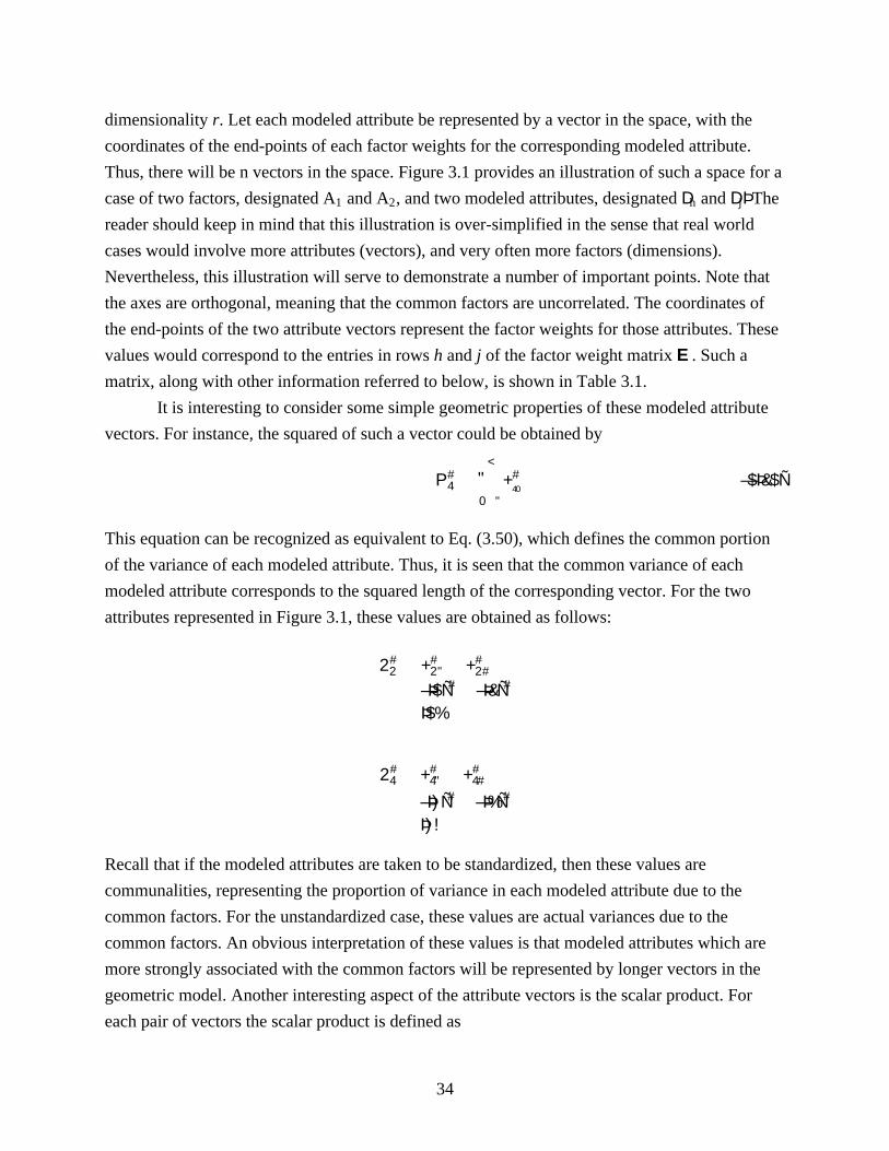
vectors. For instance, the squared of such a vector could be obtained by

P ú + Ð$Þ&$Ñ4# #

0ú"

<"40

This equation can be recognized as equivalent to Eq. (3.50), which defines the common portion

of the variance of each modeled attribute. Thus, it is seen that the common variance of each

modeled attribute corresponds to the squared length of the corresponding vector. For the two

attributes represented in Figure 3.1, these values are obtained as follows:

2 ú + Ä +

ú ÐÞ$Ñ Ä ÐÞ&Ñ

ú Þ$%

# # #2 2" 2#

# #

2 ú + Ä +

ú ÐÞ)Ñ Ä ÐÞ%Ñ

ú Þ)!

# # #4 4" 4#

# #

Recall that if the modeled attributes are taken to be standardized, then these values are

communalities, representing the proportion of variance in each modeled attribute due to the

common factors. For the unstandardized case, these values are actual variances due to the

common factors. An obvious interpretation of these values is that modeled attributes which are

more strongly associated with the common factors will be represented by longer vectors in the

geometric model. Another interesting aspect of the attribute vectors is the scalar product. For

each pair of vectors the scalar product is defined as

35

Figure 3.1: Geometric representation of two attribute vectors in a two-factor space

0.0 0.2 0.4 0.6 0.8 1.0

0.0

0.2

0.4

0.6

0.8

1.0

A1

A2

Zh

Zj

(ah1=.3, ah2=.5)

(aj1=.8, aj2=.4)

36

Table 3.1Matrices for Illustration of Transformation of Two-factor Solution

Matrix A Matrix T Matrix Φ=TT’ A1 A2 A1 A2 T1 T2

⋅

40.80.

50.30.

1

n

j

h

Z

Z

Z

Z

2

1

T

T

80.60.

28.96.

2

1

T

T

00.180.

80.00.1

Matrix T-1 Matrix B=AT-1 Matrix Q=AT’ T1 T2 T1 T2 T1 T2

2

1

A

A

−

−60.100.1

47.33.1

⋅

⋅

⋅

26.66.

1

n

j

Z

Z

Z

⋅

⋅

⋅

80.88.

1

n

j

Z

Z

Z

Matrix D=(Diag(T’-1T-1)1/2 Matrix F=DT’-1 Matrix G=AF’ F1 F2 A1 A2 F1 F2

2

1

T

T

60.00.

00.60.

2

1

F

F

−

−96.28.

60.80.

⋅

⋅

⋅

16.40.

1

n

j

Z

Z

Z

37

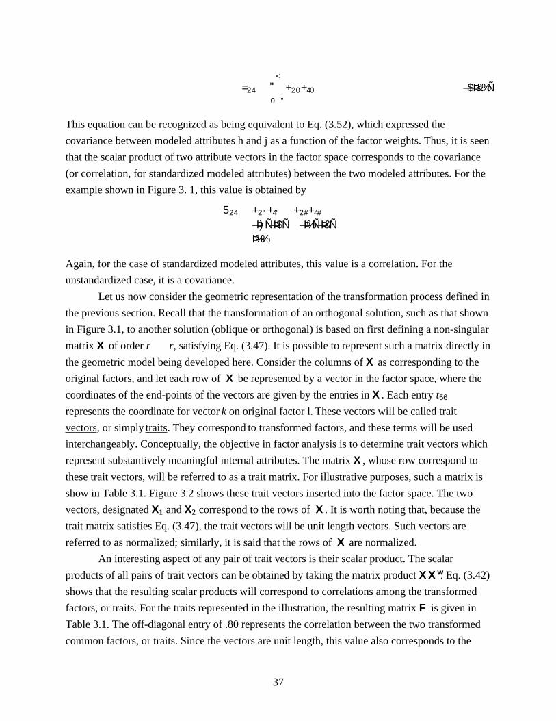
= ú + + Ð$Þ&%Ñ24 20 40

0ú"

<"This equation can be recognized as being equivalent to Eq. (3.52), which expressed the

covariance between modeled attributes h and j as a function of the factor weights. Thus, it is seen

that the scalar product of two attribute vectors in the factor space corresponds to the covariance

(or correlation, for standardized modeled attributes) between the two modeled attributes. For the

example shown in Figure 3. 1, this value is obtained by

524 2" 4" 2# 4#ú + + Ä + +

ú ÐÞ)ÑÐÞ$Ñ Ä ÐÞ%ÑÐÞ&Ñ

ú Þ%%

Again, for the case of standardized modeled attributes, this value is a correlation. For the

unstandardized case, it is a covariance.

Let us now consider the geometric representation of the transformation process defined in

the previous section. Recall that the transformation of an orthogonal solution, such as that shown

in Figure 3.1, to another solution (oblique or orthogonal) is based on first defining a non-singular

matrix of order , satisfying Eq. (3.47). It is possible to represent such a matrix directly inX r rÇ

the geometric model being developed here. Consider the columns of as corresponding to theX

original factors, and let each row of be represented by a vector in the factor space, where theX

coordinates of the end-points of the vectors are given by the entries in . Each entry X t56

represents the coordinate for vector on original factor l. These vectors will be called k trait

vectors traits, or simply . They correspond to transformed factors, and these terms will be used

interchangeably. Conceptually, the objective in factor analysis is to determine trait vectors which

represent substantively meaningful internal attributes. The matrix , whose row correspond toX

these trait vectors, will be referred to as a trait matrix. For illustrative purposes, such a matrix is

show in Table 3.1. Figure 3.2 shows these trait vectors inserted into the factor space. The two

vectors, designated and correspond to the rows of . It is worth noting that, because theX X X1 2

trait matrix satisfies Eq. (3.47), the trait vectors will be unit length vectors. Such vectors are

referred to as normalized; similarly, it is said that the rows of are normalized.X

An interesting aspect of any pair of trait vectors is their scalar product. The scalar

products of all pairs of trait vectors can be obtained by taking the matrix product . Eq. (3.42)X X w

shows that the resulting scalar products will correspond to correlations among the transformed

factors, or traits. For the traits represented in the illustration, the resulting matrix is given inF

Table 3.1. The off-diagonal entry of .80 represents the correlation between the two transformed

common factors, or traits. Since the vectors are unit length, this value also corresponds to the

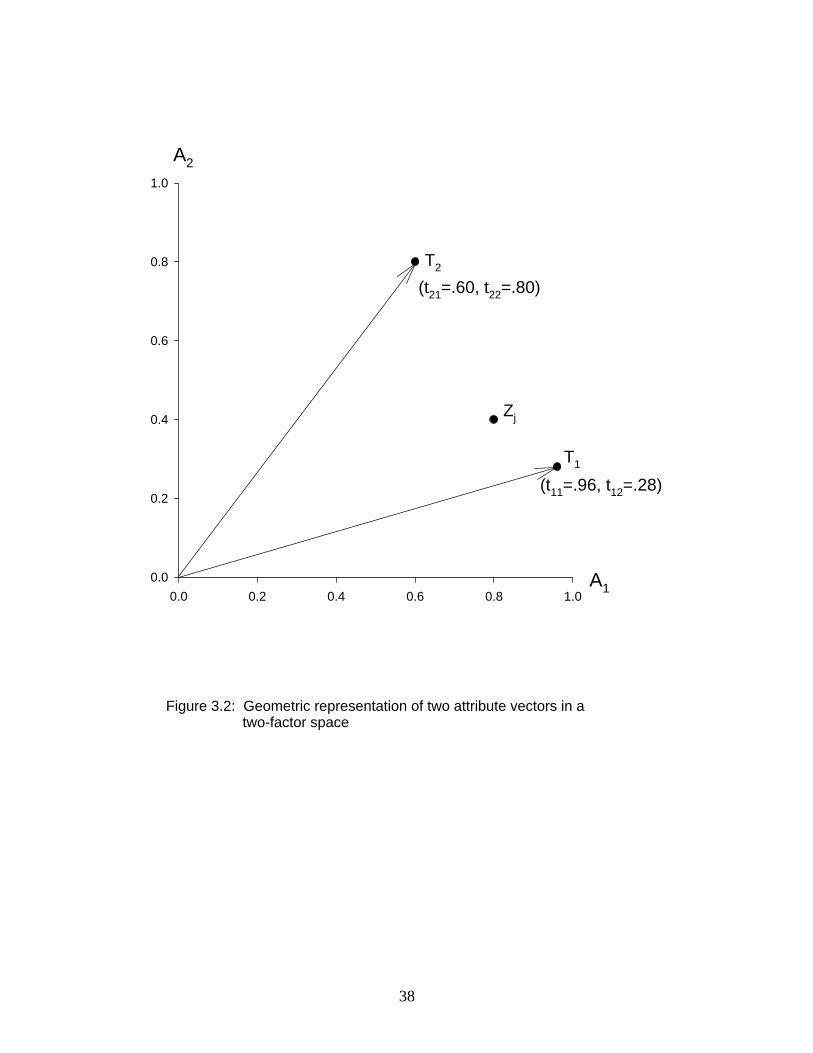
38

Figure 3.2: Geometric representation of two attribute vectors in a two-factor space

A1

A2

Zj

0.0 0.2 0.4 0.6 0.8 1.0

0.0

0.2

0.4

0.6

0.8

1.0

T1

(t11=.96, t12=.28)

(t21=.60, t22=.80)

T2

Zj

39

cosine of the angle between the two trait vectors in Figure 3.2.

We will next consider how to represent the relationships between the trait vectors and the

modeled attributes. As we will show, this can be approached in a number of different ways. One

approach has, in effect, already been defined. Eq. (3.48), repeated here for convenience, defines a

transformation of factor weights from the initial orthogonal factors to the transformed oblique

factors, or traits:

F EXú w

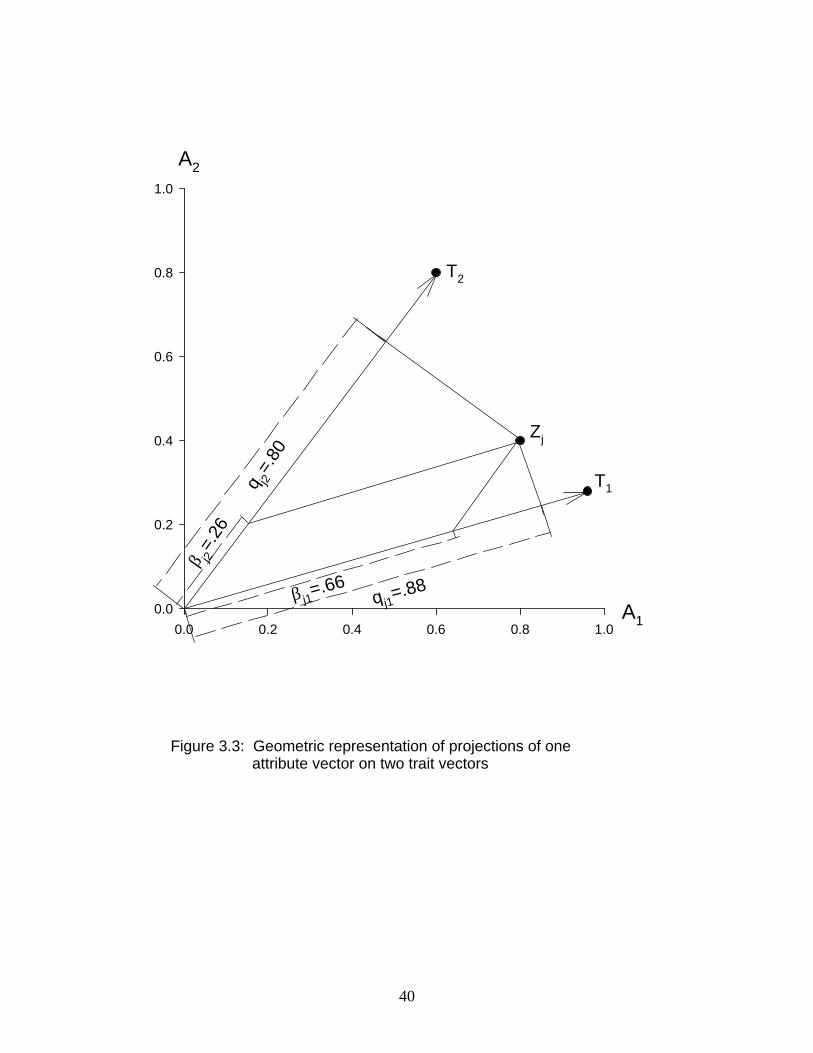
The resulting matrix contains weights for the transformed factors on the modeled attributes. InF

the geometric model, these weights correspond to the Cartesian projections of the attribute

vectors on the trait vectors. Each such weight is analogous to a partial regression coefficient,"45

representing the unique effect on modeled attribute of factor . The computation of thesej k

weights for one of the attributes is given in Table 3.1 for attribute , and the projections arej

shown in Figure 3.3.

An alternative representation of the relationships of the traits to the modeled attributes

can be obtained by determining scalar product, of the attribute vectors and the trait vectors.

Algebraically, the scalar products would be given by

U EXú Ð$Þ&&Ñw

Matrix will have rows representing the modeled attributes and columns representing theU n r

traits. Each entry will represent a scalar product, or covariance, between a modeled attributeq45

and a trait. (Again, note that for the case of standardized modeled attributes, these values will be

correlations between modeled attributes and traits). Geometrically, these values correspond to

perpendicular projections of modeled attribute vectors on trait vectors. The computation of these

values for one of the attribute vectors is shown in Table 3.1. and the corresponding projections

are shown in Figure 3.3. These projections are analogous to simple measures of covariance (or

correlation) between a modeled attribute and a trait, ignoring the fact that other traits are present.

Continuing further with the issue of evaluating relationships between modeled attributes

and traits, it has been found very useful to define a second type of vector associated with the trait

vectors. This second type of vector is based on the notion of a . Consider a solutionhyperplane

containing correlated factors. For any given factor, the remaining factors can be conceived of asr

defining a space of ( -1) dimensions. This subspace is referred to as a hyperplane. For eachr

factor, there exists a corresponding hyperplane made up of the other ( -1) factors. For each suchr

hyperplane, let us define a unit-length vector orthogonal to that hyperplane. These vectors are

called , or more simply, just . These normals are equivalent tonormals to hyperplanes normals

what Harman (1 967) and others call "reference vectors". Note that for each trait there will be a

40

Figure 3.3: Geometric representation of projections of one attribute vector on two trait vectors

A1

A2

Zj

0.0 0.2 0.4 0.6 0.8 1.0

0.0

0.2

0.4

0.6

0.8

1.0

T1

T2

Zj

q j1=.88

q j2=.

80

β j1=.66

β j2=.

26

41

corresponding normal, defined as a vector orthogonal to the corresponding hyperplane. These

normals have been used extensively in representing oblique common factor solutions.

Let us define a matrix which contains these vectors as rows. Thus, the columns ofJ Jr

correspond to the original orthogonal factors and the rows represent the normals. An entry r f56

represents the coordinate of the end-point of normal on original factor A It is useful toJ5 6Þ

consider the relationship between these normals and the traits, represented by the rows of .X

Note that each normal is defined as orthogonal to all but one trait. Therefore, if we obtain the

scalar products of the normals with the traits, as given by

X J Hw ú Ð$Þ&'Ñ

the resulting product matrix , of order , must be diagonal. This will be the case becauseH r rÇ

each normal is orthogonal to all but one trait, and vice versa. This interesting relationship can be

employed to determine a method to obtain the matrix of normals. Since the rows of areJ J

normalized vectors, this implies

H+31Ð Ñ ú Ð$Þ&(ÑJ J Mw

Solving Eq. (3.56) for yieldsJ '

J X Hw Å"ú Ð$Þ&)Ñ

Substituting from Eq. (3.58) into Eq. (3.57) yields

H3+1Ð Ñ ú Ð$Þ&*ÑHX X H MwÅ" Å"

Solving Eq. (3.59) for gives usH

H X X

X X

ú ÐH3+1Ð ÑÑ

ú ÐH+31Ð Ñ Ñ

ú ÐH3+1 Ñ

w Å"Å" "#

"#

"#

Å

w Å" Å

Å" ÅF (3.60)

This result is important because it provides a method to obtain matrix , the diagonal matrixH

containing relations between traits and normals. The diagonal elements of actually areH

equivalent to constants which serve to normalize the columns of , as shown in Eq. (3.58).XÅ"

Given the trait matrix , can be obtained according to Eq. (3.60). It can then be used to obtainX H

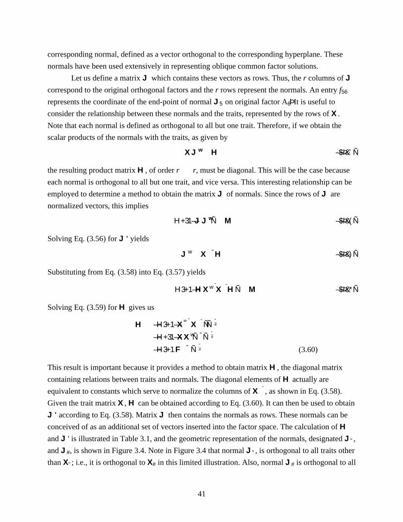
J J' according to Eq. (3.58). Matrix then contains the normals as rows. These normals can be

conceived of as an additional set of vectors inserted into the factor space. The calculation of H

and ' is illustrated in Table 3.1, and the geometric representation of the normals, designated ,J J"

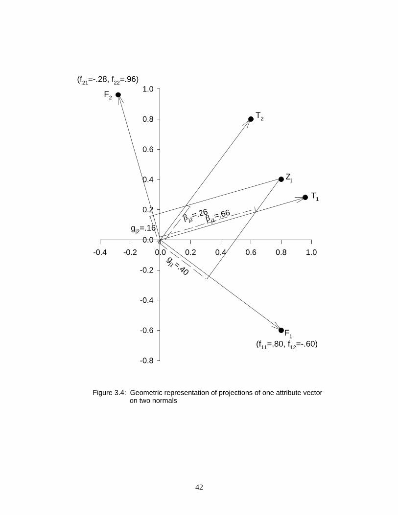
and , is shown in Figure 3.4. Note in Figure 3.4 that normal , is orthogonal to all traits otherJ J# "

than ; i.e., it is orthogonal to in this limited illustration. Also, normal is orthogonal to allX X J" # #

42

-0.4 -0.2 0.0 0.2 0.4 0.6 0.8 1.0

-0.8

-0.6

-0.4

-0.2

0.0

0.2

0.4

0.6

0.8

1.0

gj1 =.40

gj2=.16β j1

=.66β j2=.26

F1

(f11=.80, f12=-.60)

(f21=-.28, f22=.96)

F2

T1

Zj

T2

Figure 3.4: Geometric representation of projections of one attribute vector on two normals

43

traits other than ; i.e., it is orthogonal to .X X# "

The utility of these normals can be seen when we consider the relationship of the modeled

attributes to the normals. Let us define the scalar products of the modeled attributes with the

normals as

K EJú Ð$Þ'"Ñw

Matrix will be of order , with rows representing modeled attributes and columnsK n rÇ

corresponding to the normals. Each entry can be interpreted as a measure of a partialledg45

relationship. Such an entry represents the partial covariance (or correlation in the standardized

case) between modeled attribute and trait , with the effects of the other ( -1) traits partialledj k r

out. This interpretation is based on the definition of normals as being orthogonal to hyperplanes.

As such, each normal represents a partialled trait; i.e., that portion of a given trait which remains

after the effects of the other ( -1) traits are partialled out. The computation of these values isr

illustrated for a single attribute in Table 3.1. Geometrically, these values correspond to

perpendicular projections of attribute vectors on normals. These projections for a single attribute

are shown in Figure 3.4.

A very interesting relationship exists between the factor weights in matrix and theF

projections on the normals, given in matrix . Substitution from Eq. (3.58) into Eq. (3.61)K

produces

K EX Hú Ð$Þ'#ÑÅ"

Then, by substituting into this equation from Eq. (3.48), we obtain

K FHú Ð$Þ'$Ñ

According to this equation, the columns of and will be proportional. The constants ofK F

proportionality will be the diagonal elements of . Thus, the factor weights for a given factorH

will be proportional to the projections on the normals for the corresponding factor. An

examination of Figure 3.4 reveals the geometric basis for this relationship. Note that the

projection of a given modeled attribute on a normal in this example is obtained by "continuing"

the projection from the attribute, through the trait, to the normal. The Cartesian projections of the

attribute vectors on the trait vectors were illustrated originally in Figure 3.3. These same

projection are shown also in Figure 3.4, which illustrates how those projections are related to the

projections of the attribute vectors on the normals. This gives rise to the proportionality defined

in Eq. (3.63)

To summarize the developments presented in this section, begin with the assumption that

an orthogonal solution characterized by matrix has been obtained. Given such a solution, aE

44

transformation then can be carried out by defining a trait matrix , the rows of which representX

the traits, or transformed factors. One then can obtain, by equations presented above, matrices ,F

containing the correlations of the factors; , containing the factor weights; , containing theF U

covariance of the modeled attributes with the factors; and , containing the partialledK

covariances of the modeled attributes with the factors. In the geometric representation of the

model, the modeled attributes are represented by vectors in a space whose axes correspond to the

initial orthogonal factors. The transformed factors are represented by trait vectors, defined by the

rows of matrix . The correlations among the trait vectors, contained in matrix , correspondsX F

to cosines of angles between the trait vectors. The factor weights in matrix correspond toF

Cartesian projections of the attribute vectors on the trait vectors. The covariances of the modeled

attributes, with the trait vectors, contained in matrix , correspond to perpendicular projectionsU

of the attribute vectors on the trait vectors. Finally, the partialled covariance of the modeled

attributes with the trait vectors, contained in matrix , correspond to projections of the attributeK

vectors on normals to the hyperplane defined by each trait vector. These matrices define an

oblique common factor solution.

It is important to recognize the properties of such a solution when the traits themselves

are orthogonal. That is, consider the case in which

X X Mw ú Ð$Þ'%Ñ

Under this condition, is equivalent to . As a result, matrix as defined in Eq. (3.48) willX X Fw

be equivalent to matrix as defined in Eq. (3.55). In addition, the matrix as defined in Eq.U H

(3.60) will be an identity matrix. As a result, Eq. (3.63) shows that and will be equivalent.F K

The implication of these relationships is that when the traits are orthogonal, there will be no

distinction among matrices , , and . All of the types of information contained in theseF KU

matrices will be equivalent in this case. In geometric terms, this phenomenon is revealed by the

fact that when the traits are orthogonal, there will be no distinction between Cartesian projections

(as given in ) and perpendicular projections (as given in ) of the attribute vectors on the traitF U

vectors. Furthermore, each normal will be equivalent to the corresponding trait vector, since the

trait vectors themselves are orthogonal to the hyperplanes. Thus, the projections on the normals

(given in ) will be equivalent to the projections on the trait vectors. This all demonstrates thatK

an orthogonal solution is, in some senses, simpler than an oblique solution, since there are no

trait correlations to consider and since the types of relationships between attributes and traits are

all equivalent. However, as will be discussed in Chapter 9, this relative simplicity should not be

considered to represent an advantage of orthogonal solutions over oblique solutions. The critical

issue is to determine traits which correspond to substantively meaningful internal attributes,

whether or not they are or orthogonal.

45

3.4. Effects of Factor Transformations on Factor Scores

A recurring theme in the previous three sections has been the transformation of factors.

Mathematical and geometric frameworks have been described for representing the transformation

of common factor weight matrices. It is very important that the reader recall the role of these

factor weights in the common factor model. According to the model as defined in Eq. (3.7) or Eq.

(3.39), these weights are weights which are applied to scores on the common factors. The

resulting linear combination of common factor scores, combined with specific factor and error of

measurement factor terms, yield the modeled attributes. Let us focus at this point on the common

factor contribution to the modeled attributes. Given the nature of the model, it is clear that any

transformation of the common factor weights must also imply a corresponding transformation of

the common factor scores. To put this more simply, if some operation is carried out to alter the

common factor weights in model expressed in Eq. (3.7) or Eq. (3.39), then the common factor

scores must also be altered in order that the model still produce the same modeled attributes. In

this section we will present a framework for representing this phenomenon, and we will consider

a number of related issues of both theoretical and practical importance.

To begin, let us consider Eqs. (3.7) and (3.39). In these expressions of the model, the

common factor contributions to the modeled attribute scores in are contained in the productD

B D"F'. Let us define a vector . as containing these contributions. That is-

D B-wú Ð$Þ'&Ñ"F

As described in sections 3.2 and 3.3, let us consider to be a transformed matrix of factorF

weights. Suppose that an initial orthogonal weight matrix had been obtained, and that is theE F

result of transforming according to Eq. (3.48). Substituting from Eq. (3.48) into Eq. (3.65)E

yields

D B-w wú "X EÅ"

Ð$Þ''Ñ

Let us define a vector as follows:B!

B B! "ú X wÅ"

Ð$Þ'(Ñ

Substituting from this equation into Eq. (3.66) yields

D B-wú !E Ð$Þ')Ñ

A comparison of Eqs. (3.65) and (3.68) indicates that these provide two different representations

of the scores, based on two different factor weight matrices. Thus, it can be seen that D B- "

46

contains the common factor scores corresponding to the weights given in , and contains theF B!

common factor scores corresponding to the weights given in . Furthermore, Eq. (3.67)E

represents the transformation between the two sets of common factor scores.

It is interesting to consider also the covariance among the factor scores. The covariance

among the factor scores in are given by which is defined in Eq. (3. 10) as matrix , theB" ""D , F

intercorrelation matrix for the common factors. In the present section, we will employ an

additional level of subscripts and will designate this matrix as Eq. (3.67) defines a linearDB B" "

.

transformation relating Based on such a transformation, the relation between theB B" !to .

covariance matrices for these two sets of common factor scores can be obtained by employing

Corollary 3 of Theorem 4 in Appendix C. This yields the following:

D DB B B Bw

! ! " "ú X X

Å" Å"

Ð$Þ'*Ñ

Since is designated as , and since is identified in Eq. (3.42) as being equal to ,DB B! !F F X X '

Eq. (3.69) can be rewritten as follows:

DB Bw w

! !ú X X X X

Å" Å"

Ð$Þ(!Ñ

This shows that the covariance matrix for the common factor scores corresponding to the

orthogonal weight matrix will be an identity matrix; i.e., these common factor scores will beE

uncorrelated.

A geometric representation of these relations is of interest. Let us consider a geometric

framework of a different nature than that employed in section 3.3. In particular, let us define a

factor score space in terms of the factor scores given in . The axes in this space represent theB!

common factors, and each individual will be represented by a point in the space, with the

coordinates of each individual's point being given by the common factor score vector, , forB!

that individual. Equivalently, each individual can be thought of as being represented by a vector

in the factor score space, with the coordinates of the endpoint of each individual's vector being

defined by the scores for that individual on the common factors. Note that, according to Eq.

(3.70) the distribution of points in the space will be such that the scores on the original axes will

be standardized and uncorrelated. Let us next consider the representation of the scores on the

transformed factors, given in Employing Eq. (3.67), we can obtain the following relation:B" .

B B" !ú X w Ð$Þ("Ñ

This equation indicates that the factors scores in are scalar products of the scores in withB B" !

the trait vectors in . Since the trait vectors are of unit length, these scalar products correspondX

to projections of the vectors on the trait vectors. The correlations among the factor scores inB!

47

B" , which are given in , are cosines of angles between the trait vectors. A point of considerableF

importance is that the relations among the factors are defined in this factor score space.

An interesting special case of the transformation problem is the transformation from one

uncorrelated solution to a second such solution. Let us examine the impact of such a

transformation on the factor scores and their interrelationships, employing the mathematical

framework developed above. In this case, will be defined such thatX

X X Mw

ú Ð$Þ(#Ñ

This implies that

X Xw ú Ð$Þ($ÑÅ"

Let be the weight matrix for the first uncorrelated solution and be the weight matrix forE E" #

the second such solution. By Eq. (3.48)

E E X# "wú Ð$Þ(%Ñ

Let the factor scores corresponding to be given by , then by using Eqs. (3.68), (3.73), andE" "B!

(3.74), we can obtain the following:

D B B- " "" #wú ú! !E X Ew w Ð$Þ(&Ñ

Let the scores on the second solution be given by , which according to Eq. (3.71), would beB!2

given by

B B! !2 ú "wX Ð$Þ('Ñ

Employing Eqs. (3.75) and (3.76), we obtain the following:

D B B- " " #w wú ú! !E E2 Ð$Þ((Ñ

This equation simply shows that both sets of common factor scores and weights produce the

same values. It also can be shown that the covariance matrices for the two sets of factor scoresD-

have the expected form. Making use of the linear transformation defined in Eq. (3.74) along with

Corollary 3 of Theorem 4 in Appendix C, we obtain the following:

D DB B B Bw

+ +# +" +2 1ú X X Ð$Þ()Ñ

Since the initial solution defined as orthogonal, we can writeE" is

DB B+" +1 ú M Ð$Þ(*Ñ

Substituting from Eqs. (3.79) and (3.72) into Eq. (3.78), we obtain

48

DB Bw

+ +#2 ú úX X M Ð$Þ)!Ñ

Thus, both solutions are characterized by factor scores which are standardized and uncorrelated.

We wish to consider next a very interesting issue which often gives rise to substantial

confusion in empirical applications of factor analysis. The issue concerns the nature and meaning

of product matrices obtained by pre-multiplying factor weight matrices by their respective

transposes. A common misconception is that the relations among the common factors are

represented in such matrices. Let us first consider this issue in the context of the special case just

described--the transformation of one orthogonal solution into a second such solution LetE E" #.

us define product matrices as follows:T T" # and

T E E" ""wú Ð$Þ)"Ñ

T E E# ##wú Ð$Þ)#Ñ

Substituting from Eq. (3.74) into Eq. (3.82) yields

T X T X# "wú Ð$Þ)$Ñ

The misconception involves the issue of whether the relations among the common factors are

indicated by the entries in Suppose is diagonal and the diagonal entries areT T T" # " and .

unequal (this is a property of a particular type of solution, called a principal factors solution, to

be described in Chapter 7). According to Eq. (3.83), generally will not be a diagonal matrix.T#

That is, even though the transformed solution represented by is an orthogonal solution, theE#

product matrix generally will not be diagonal. This is a point which troubles manyT#

practitioners of factor analysis. How can be an orthogonal factor matrix when its columns areE#

not "orthogonal"? The resolution of this apparent paradox was given earlier in this section: the

orthoganality of the factors is defined in the factor score space, and is not defined by product

matrices such as That is, the factor scores for the factors defined by are uncorrelated, asT E# #.

shown in Eq. (3.80), even though matrix is not diagonal.T#

Let us consider this issue in the more general context of transformations from

uncorrelated factors to correlated factors. Eq. (3.71) defines the impact of such a transformation

on the factor scores. The area of concern here is with the product matrices, which will be

designated as follows:

T E E! ú w Ð$Þ)%Ñ

49

T F F" ú w Ð$Þ)&Ñ

Employing Eq. (3.48), we can rewrite Eq. (3.85) as follows:

T X E EX" ú w wÅ" Å"

Ð$Þ)'Ñ

Substituting from Eq. (3.84) into Eq. (3.86) yields

T X T X" !ú wÅ" Å"

Ð$Þ)(Ñ

This equation gives the transformation of The inverse transformation is implied. TheT T! " to .

critical aspect of Eq. (3.87) is that it shows that there is no necessary, direct relation of to .T" F

That is, matrix defines the relations among the common factors, and the relations are notF

indicated in any way in matrix T" .

An illustration of the distinction between and involves a type of solution called anT" F

independent cluster solution. In this case, each modeled attribute has a non-zero weight on one

and only one factor in B. In such a case, would be diagonal since the sums of productsT"

between columns of would be zero. However, matrix would not necessarily be diagonal.B F

The independent clusters of attributes might be intercorrelated so that would have non-zeroF

off-diagonal entries.

To complete the discussion of this issue, let us consider four possible situations defined

by combining the possibilities of being diagonal or not diagonal. When both are diagonal, theF

solution would be a principal factors solution; this type of solution was mentioned earlier in this

section and will be discussed in detail in Chapter 7. The other cases can be thought of as arising

from various possible transformations of such a solution. The case where is diagonal and F T"

is not diagonal would be produced by an orthogonal transformation of a principal factor solution.

This is a legitimate view since any factor solution could be transformed into a principal factors

solution. The case where is not diagonal and is diagonal would be produced by certainF T"

special transformations from a principal factors solution, including a transformation to an

independent cluster solution. Finally, the case where is not diagonal and is not diagonalF T"

represents the more general case of transformation to a general oblique solution.

This completes our discussion of the effects of factor transformations on factors scores.

Critical points to keep in mind are that transformations of factor weights imply corresponding

transformations of factor scores., and that the relations among the factors are defined in the factor

score space. It is a misconception to consider the relations among the factors as being defined by

the factor weights themselves.

50

3.5. Correspondence Between the Model and the Real World

An issue emphasized in Chapter 1 and in the first section of the present chapter involves

the correspondence between the common factor model and the real world. It is recognized that

we do not expect the model to provide an exact and complete accounting for the variance and

covariances of the surface attributes. This fact is represented in the mathematical framework by

differentiating between the surface attributes (vector ) and that portion of the surface attributesC

that is consistent with the common factor model (the "modeled attributes" in vector ).D

According to the mathematical representation of the model defined in this chapter, the model

does account for the variances and covariances of the modeled attributes. That is, the covariance

matrix is a function of the parameters of the model, as shown in Eq. (3.35).DDD

It is important to represent explicitly the fact that, though the model accounts for the

variances and covariance of the modeled attributes, it will not necessarily do the same for the

surface attributes themselves. This can be seen by defining a population covariance matrix DCC

for the surface attributes. Matrix will be of order , with entries ng theDCC n nÇ 524 representi

population covariance for surface attributes and . It is especially important to consider theh j

relation between This can be done by making use of the fact, as defined inD DCC DD and .

Eq. (3.1), that the surface attributes in are actually sums of the component portions in and .C z z..

Appendix C treats the case where one vector of measures is defined as the sum of two other

vectors of measures, and shows the relationship of the covariances of the summed measures to

those of the component portions. By applying the relationship shown in Theorem 5 of Appendix

C, we can write, for the present case, the following:

D D D D DCC DD DD DD DDú Ä Ä Ä.. .. .. .. Ð$Þ))Ñ

From this equation it can be seen clearly that the population covariance matrix for the

surface attributes is not, in general, equivalent to the population covariance matrix for the

modeled portions of the attributes. More specifically, if we define a matrix as?D

? D D DD ú Ä ÄDD DD DD.. .. .. .. Ð$Þ)*Ñ

then Eq. (3.88) can be re-written as

D D ?CC DDú Ä D Ð$Þ*!Ñ

The matrix then represents that portion of the population covariances of the surface attributes?D

that cannot be accounted for by the common factor model. It can then be seen that only when all

entries in are zero will be equivalent to In that situation, the model will exactly? D DD CC DD .

represent the population covariances for the surface attributes. But if some entries in are not?D

zero, then will not be equivalent to , and the model will not hold exactly in theD DCC DD

51

population. As the entries in deviate further from zero, the correspondence between the?D

model and the population becomes weaker. This lack of correspondence between the model and

the real world is a very important concept which is often overlooked by neglecting the distinction

between and We will refer to such lack of correspondence as , meaning that theC D. model error

representation of the real world by the model is in error to some degree. It must be understood

that model error is and is completely separate from lack of fit arisingpresent in the population

from sampling. That is, even if there is no model error, meaning that the model holds exactly in

the population, there still will be sampling error. That is, the model probably would not fit a

sample covariance matrix exactly. This issue will be dealt with further in Chapters 4 and 5.

A final step in developing the common factor model in the population now can be

achieved by substituting from Eq. (3.35) into Eq. (3.90). This yields

D F ?CCw #ú Ä ÄF F Y D Ð$Þ*"Ñ

This equation represents the milestone of expressing the common factor model in terms of the

population covariances of the . This expression represents these covariances as asurface attributes

function of the parameters in , , and plus a term representing model error. MostF YF #,

presentations of the model ignore the need to explicitly include model error.

The presence of model error can serve as a basis for introducing the concept of fitting the

model to a covariance matrix. Considering the hypothetical case where a population covariance

matrix is available, suppose we wish to obtain a solution for the model as represented in Eq.DCC

(3.91). Recognizing that represents the lack of fit of the model to , the objective would? DD CC

be to obtain a solution for the model which, in some sense, minimizes the entries in Such a?D.

solution would be optimal in the sense of providing the most accurate accounting of the

population covariances of the surface attributes. As it will be seen in Chapter 7, there are

different ways to define the optimal solution; i.e., different ways to define a criterion representing

an optimal These alternative definitions of an optimal solution in turn lead to alternative?D.

techniques for obtaining a solution to the model, and these alternative techniques can yield

different solutions. In other words, there may be no single correct solution. Rather, different

definitions of an optimal solution yield different , , and matrices, and, in turn, differentF YF #

D ? ?DD and D Dmatrices. Only when a solution can be found for which all entries in are zero

can it be said that the model is consistent with the real world; in that case, there would be no

model error.

Surely, however, almost all acceptable models will not fit the real world perfectly in the

population. To insist on a perfect fit at all times is a route to chaos by the inclusion of many

small, trivial factors. To be sure, we should avoid missing small factors which can be made large

and important with special studies. All experimenters should be alert to this possibility. The

52

distinction between trivia and important small influences is a matter for experimenter insight and

judgment. However, the complexities of factor analysis make it imperative that a distinction be

made. Inclusion of a number of very small factors in an analysis results in unmanageably large

dimensionality of the common factor space. Great care is required of an experimenter in making

the decision between possibly meaningful factors and trivia. There should be no doubt but that

some trivia will exist.

3.6. The Common Factor Model for a Population Correlation Matrix

The development of the common factor model in this chapter has been carried out in the

context of covariance matrices. That is, the fundamental reputation of the model given in

Eq. (3.91) was stated in terms of a population covariance matrix for the surface attributes. Since

many applications of factor analysis are conducted using correlation matrices rather than

covariance matrices, it is important to consider how the expression of the model is affected when

the data are correlations rather than covariances. This can be achieved easily by employing the

simple relation between a covariance matrix and a correlation matrix. Given a population

covariance matrix for the surface attributes, , let us define a diagonal matrix D DCC . CCÒ Ó

containing the population variances of the surface attributes. That is,

Ò ÓD D. CC CCú H3+1Ð Ñ Ð$Þ*#Ñ

We can then define a population correlation matrix for the surface attributes, , as follows:VCC

V Ò Ó Ò ÓCC . CC .Å ÅCC CCú D D D

" "# # Ð$Þ*$Ñ

The effect of this standardization of the surface attributes on the common factor model can then

be seen by substituting from Eq. (3.91) into Eq. (3.93), yielding

V Ò Ó F F Y Ò Ó

Ò Ó F F Ò Ó Ò Ó Y Ò

CC . .Å Åw #

CC

. . .Å Å ÅCC CC

w #

ú Ð Ä Ä Ñ

Ä

D F ? D

D F D D D

" "# #

" " "# # #

CC

CC

D

ú .Å

. .Å ÅCC CC

Ó

Ò Ó Ò Ó

"#

" "# #

CC

Ä Ð$Þ*%ÑD ? DD

To simplify this expression, let us define the following matrices:

Fá ú Ð$Þ*&ÑÒ Ó FD.ÅCC

"#

Y á#

ú Ð$Þ*'ÑÒ Ó Y Ò ÓD D. .Å ÅCC CC

#" "# #

53

? D ? DV . .Å ÅCC CCú Ò Ó Ò Ó

" "# #

D Ð$Þ*(Ñ

Substituting from these three equations into Eq. (3.94) yields

V F F YCC Vá á áwú Ä ÄF ?

#

Ð$Þ*)Ñ

This is an expression for the common factor model in terms of a population correlation matrix

for the surface attributes. It has the same general form as Eq. (3.91), which expressed the model

in terms of a population covariance matrix, but some of the terms in the equation have been

rescaled. Note that, according to Eq. (3.95), the common factor weights obtained from a

population covariance matrix would be rescaled in that each row of would be divided by theF

population standard deviation of the corresponding surface attribute to yield the rows of .Fá

Matrix would contain the common factor weights obtained from a population correlationFá

matrix or, equivalently, from surface attributes standardized in the population. Note that the

common factor intercorrelations, given in , are not affected by this standardization. The uniqueF

variances, though, do undergo a rescaling, as shown in Eq. (3.96). The unique variances resulting

from this rescaling represent population unique variances that would be obtained from a factor

analysis of a population correlation matrix. Based on Eq. (3.16), corresponding population

common variance, would be defined as follows:

L F Fá á á# w

ú H3+1Ð ÑF Ð$Þ**Ñ

Employing Eqs. (3.16) and (3.95), this could be rewritten as follows:

L Ò Ó L Ò Óá #. .

Å ÅCC CC

# " "# #ú D D Ð$Þ"!!Ñ

This shows how the population common variances are rescaled when they are obtained from a

factor analysis of a population correlation matrix rather than a covariance matrix. It is important

to understand the distinction between two sets of matrices: and defined in Eqs. (3.96)Y Lá á# #

and (3.100), versus defined in Eqs. (3.33) and (3.25). Both sets of matrices representY Lµ µ

# # and

rescaling of , which contain the population unique and common variances,Y L# # and

respectively. However, the rescalings are slightly different. Matrices are obtained byY Lµ µ

# # and

dividing entries in and by the population variances of the modeled attributes, thusY L# #

yielding the population uniquenesses and communalities. On the other hand, matrices andY á#

L Y Lá # ## are obtained by dividing entries in by the population variances of the surface and

attributes. This operation merely rescales the variance components so that they represent surface

attributes standardized in the population. It is interesting to note that in general Y Lá á# # and

will not sum to an identity matrix because some of the population variance of the standardized

surface attributes will arise from error of fit of the model. Finally, to complete the discussion of

54

Eq. (3.98) above, the matrix represents model error in the population correlation matrix and?V

is defined by Eq. (3.97) via a rescaling of ?D.

In sum, these developments show that the analysis of population correlation matrices

rather than population covariance matrices results in a rescaling of factor weights, unique

variances, and the model error term, but does not affect common factor intercorrelations. Further

theoretical and practical implications of the issue of analysis of correlation vs. covariance

matrices will be discussed in subsequent chapters. We will continue to present major

developments in the context of covariance matrices and to consider the analysis of correlation

matrices as a special case.

3.7. The Components Analysis Model

In the previous sections in this chapter we have presented the algebraic and geometric

representation of the common factor model. There exists a variation of this model which is

commonly used in practice. This alternative approach is called . Thoughcomponents analysis

components analysis is often viewed as a variety of factor analysis, and in fact is often called

factor analysis in the applied literature, it is important to recognize it as a distinct model and to

understand how it is different from the common factor model.

In mathematical terms, the components analysis model can be defined by eliminating

specific and error of measurement factors from the common factor model. Thus, if we delete the

specific and error of measurement factors from Eq. (3.7), we obtain

D Bú "Fw Ð$Þ"!"Ñ

In terms of covariance matrices, we could write an oblique components model bymodifying

Eq. (3.35) to obtain

D FDDwú F F Ð$Þ"!#Ñ

In a similar fashion, Eq. (3.45) could be modified to yield an orthogonal components model as

follows:

DDDwú EE Ð$Þ"!$Ñ

As represented in Eq. (3.72) the components model states that modeled attributes are linear

combinations of underlying dimensions. These dimensions will be called components and mustr

be distinguished from common factors. Recall that a common factor represents a substantively

meaningful internal attribute which affect more than one attribute in the battery and which

partially explains why surface attributes are correlated. It is essential to recognize that the

mathematical representation of common factors requires that specific and error of measurement

55

factors be represented separately, since the latter represent real phenomena which influence the

attributes in a manner different from the common factors. Since the components model does not

provide for these specific and error of measurement factors, the components in this model cannot

be considered to be conceptually the same thing as common factors. This is due to the fact that

the components will represent not only common variance, but also specific and error of

measurement variance. Furthermore, it will not be possible to differentiate these various

influences in a components solution.

Nevertheless, components analysis has often been used in practice and viewed as

equivalent to, or at least an acceptable substitute for, common factor analysis. Supporters of this

position tend to base their view on several points. The relative simplicity of the components

model often is considered to be an advantage over factor analysis. The absence of specific and

error of measurement factors from the model simplifies the process of fitting the model to the

data in that it eliminates the need to estimate the unique influences. In addition, it is often argued

that components analysis solutions are often found to be quite similar to common factor

solutions. Finally, the major argument used for support of the components model is that it is

possible to determine exactly the measures for the individuals on the components (i.e., the entries

in in Eq. (3.101). This is not the case in the common factor model; that is, the measures for theB

individuals on the common factors, contained in vector in Eq. (3.7), cannot be determinedB

exactly. These scores are said to be "indeterminate", and can only be estimated. Component

scores, on the other hand, are determinate. These arguments have led many researchers to view

components analysis as holding advantages over common factor analysis.

Our view, however, is that these arguments carry very little impact. Let us consider them

in turn. First, though it is true that the components model is simpler, it must be recognized that

this simplicity is gained at the cost of the realism of the model. The common factor model offers

a much more realistic representation of attributes in that it explicitly recognizes and incorporates

the existence of specific and error factors. The fact that such influences are ignored in the

components model yields a simpler but very unrealistic model. Furthermore, this simpler model

yields dimensions which, as pointed out above, cannot be conceived of as representing

substantively meaningful common factors. Considering the argument that components solutions

often closely approximate common factor solutions, this will be the case under certain

conditions. It can be seen easily by comparing Eqs. (3.102) and (3.103) to Eqs. (3.36) and (3.45),

respectively, that as the unique variances of the attributes become smaller the two models

become more similar. When unique variances are zero, the two models are equivalent. However,

when substantial unique variances are present, solutions obtained from the two models may not

be very similar. Thus, the argument that solutions from the two models are quite similar will not

hold under all conditions. Finally, considering the issue of indeterminacy, we do not consider this

56

as a fatal flaw in the common factor model for two reasons. First, as emphasized in Chapter 1,

the objective of obtaining measures for the individuals on the common factors is not, in our view,

a primary objective of factor analysis. The primary objective is to obtain an understanding of the

nature of the common factors and the manner in which they influence the attributes. Given this

view, the fact that the measures on the common factors are indeterminate is not a serious

problem. Furthermore, as will be shown in Chapters 15 and 16, when a researcher does have a

legitimate need for the scores on the common factors, there are procedures for estimating those

scores, and to estimate them in such a way as to negate some of the effects of indeterminacy.

In summary, our view is that the components model is unrealistic and is not an acceptable

substitute for the common factor model. Though there is an indeterminacy problem in the

common factor model, this problem is not serious and can be dealt with when common factor

scores are desired. This problem does not involve the central objective of factor analysis. In

general then, we strongly oppose the use of components model and do not recommend it in

practice. We support the use of the common factor model because it is based on a more realistic

representation of the structure of the attributes and their relationships and because it offers a

better chance to obtain an undergoing of the nature of the common factors and their effects on the

attributes.

3.8. The Issue of Linearity

The common factor model is commonly referred to as a model. It is most importantlinear

to achieve an understanding of the sense in which the model is linear. Let us consider three types

of relationships which are relevant to the model: relationships of modeled attributes to each

other; relationships of factors to each other; and relationships of modeled attributes to factors.

As defined in Eq. (3.7), the model states that the modeled attributes are linear

combinations of the factors. If, in the real world, the surface attributes are non-linear functions of

the factors, these relationships cannot be explicitly represented by the linear common factor

model. In such a situation, the population covariance matrix for the surface attributes, , couldDCC

not be perfectly represented by the model. That is, given it would not be possible to find aDCC,

solution such that all entries in matrix , defined in Eq. (3.89), would be zero.?D

It is important to recognize, however, that the model makes no statement, either implicit

or explicit, about the linearity of the relationships of the attributes to each other, or the factors to

each other. In fact, the relationships can be non-linear. It is possible for the attributes to have

non-linear relationships to each other, and for the factors to have non-linear relationships to each

other, and for the model still to exactly represent the population covariance matrix for the surface

attributes. This would simply require that the surface attributes be linear functions of the factors.

57

Two demonstrations will be presented to illustrate the points made here. The general

procedure used in these demonstrations involves first constructing artificial data representing a

population. That is, a population covariance matrix for surface attributes will be constructed such

that the underlying relationships among attributes and factors have the desired properties of

linearity or non-linearity. A common factor solution then will be obtained (by procedures to be

described in Chapter 7) which fits the population covariance matrix as well as possible. It is not

necessary for the reader to understand, at this point, the methodology for obtaining such a

solution. The key issue in these demonstrations will be to determine whether or not the obtained

solution fits the population covariance matrix perfectly; i.e., whether the matrix contains all?D

zeroes. If this is the case, then the linear factor model holds in the population; if not, then the

relationships among the surface attributes cannot be represented exactly by the linear factor

model.

The first demonstration is designed to show the effects of curvelinear relations among

factors and among attributes. A population distribution of measures on two common factors was

defined such that the relationship between the factors was curvelinear. This distribution is shown

in Figure 3.5. In this figure, the axes represent two common factors. Each individual in the

population was defined as falling at one of 25 discrete points, represented by the centers of the

circles in the space. The values in the circles represent relative frequencies of observations at

each corresponding point. The resulting distribution represents a population distribution of

measures on two factors which are related in a curvelinear fashion. Scores on both factors had a

mean of .644 and a standard deviation of .302; note that these original factors are unstandardized.

The correlation between these factors was -.762. Each observation draw from this distribution

would provide a vector of measures on common factors.B

Next a population factor weight matrix was defined. This matrix is presented inF

Table 3.2. Matrix contains weights for the two unstandardized factors on 10 artificiallyF

defined attributes. Table 3.2 also includes the factor weight matrix which would be applied to

standardized factor scores. These weights are obtained by multiplying each column of original

factor weights by the standard deviation of the factor (.302). It is important to note that the

weights were defined in such a way that attribute 1 is equivalent to factor 1 and attribute 10 is

equivalent to factor 2. As a result, the relationship of attributes 1 and 10 will be identical to that

represented in Figure 3.5. That is, in addition to there being a curvelinear relationship between

the factors, there also will be a curvelinear relationship between attributes 1 and 10 (as well as

other pairs of attributes).

Measures on two common factors for a hypothetical population of 100 individuals were

generated so as to follow the distribution shown in Figure 3.5. Population measures on the

surface attributes then were obtained according to Eq. (3.7). For simplicity, no specific or error

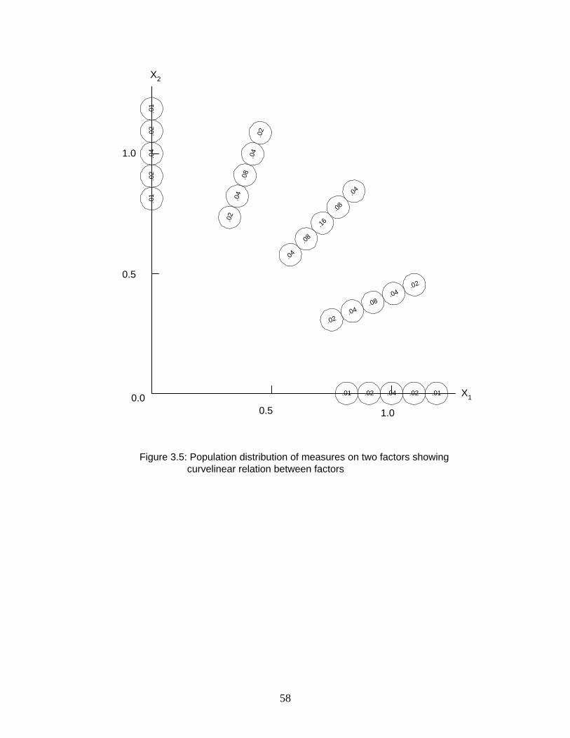
58

1.00.5

X1.04 .01.02.01 .02

.04

.01

.02

.01

.02

.16

.04

.08

.04

.08

0.5

.08

.02

.04

.02

.04

.08

.02

.04

.02.04

X2

0.0

1.0

Figure 3.5: Population distribution of measures on two factors showing curvelinear relation between factors

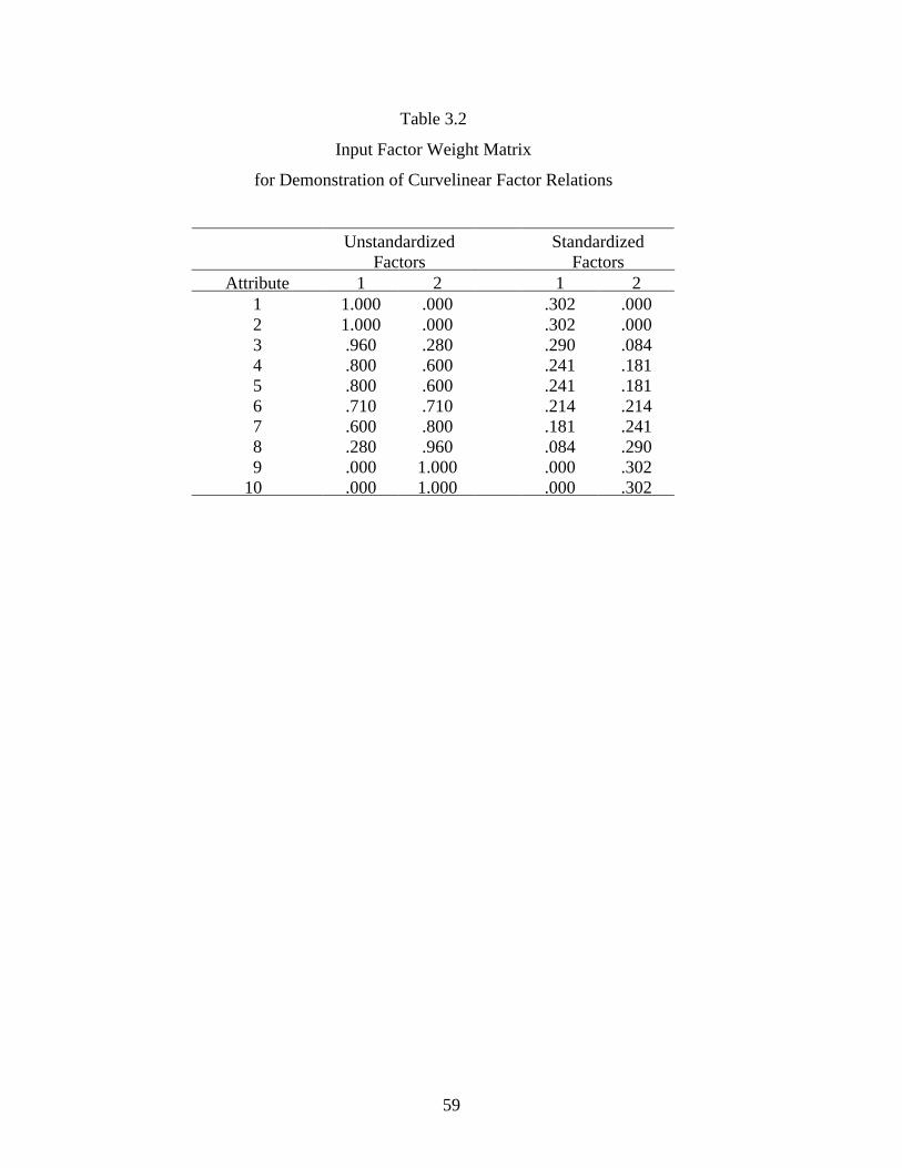
59

Table 3.2

Input Factor Weight Matrix

for Demonstration of Curvelinear Factor Relations

UnstandardizedFactors

StandardizedFactors

Attribute 1 2 1 21 1.000 .000 .302 .0002 1.000 .000 .302 .0003 .960 .280 .290 .0844 .800 .600 .241 .1815 .800 .600 .241 .1816 .710 .710 .214 .2147 .600 .800 .181 .2418 .280 .960 .084 .2909 .000 1.000 .000 .302

10 .000 1.000 .000 .302

60

factors were included in the demonstration. Thus, the surface attributes were defined as linear

combinations of the common factors, with the weights given in matrix . Next, a populationF

covariance matrix for the surface attributes was computed from the population of measures on

those attributes. The resulting matrix is presented in Table 3.3. Note that this covarianceDCC

matrix has been produced from a case where there exist curvelinear relations among factors and

among attributes, but the relations of the attributes to the factors are linear.

A factor solution then was obtained (via procedures to be discussed in Chapter 7). This

yielded a solution containing two factors. The resulting orthogonal factor weight matrix is shown

in Table 3.4. Considering this as matrix , it was found that the resulting matrix producedE DDD

via Eq. (3.45), recalling that unique variances are zero in this demonstration, was identical to the

population covariance matrix in Table 3.3. In other words, the matrix , whose entriesD ?CC D

represent lack of correspondence between the model and the population, contained all zeroes.

Furthermore, it was found that the orthogonal solution represented by matrix in Table 3.4E

could be transformed to match the original input factor weights given in Table 3.2. Note that

since the obtained factor weights represent standardized factors, the transformation of the

obtained solution should yield the input weights for standardized factors. Following the

procedures in section 3.3 above, this transformation was achieved by passing the first trait vector

and the second trait vector through the last attribute vector. The resulting trait matrix is shownX

in Table 3.4. Based on this trait matrix, we then obtained the intercorrelation matrix and theF

weight matrix for the transformed factors by Eqs. (3.42) and (3.44), respectively. The resultingF

matrices are shown in Table 3.4 and can be seen to be identical to the corresponding input

information. These findings of perfect fit and exact recovery of the input factors indicate that the

linear factor model holds exactly in this population, despite the presence of curvelinear relations

among factors and among attributes. The fact that the relations of the attributes to the factors are

linear allows for this perfect correspondence between the factor model and the population.

The second demonstration involves the case of curvelinear relations of attributes to

factors. This demonstration makes use of "binary" attributes; i.e., attributes which can take on

only two possible values. The most common example of such an attribute is a test item, where

responses to the item are scored as correct (1) or incorrect (0). Such items are very commonly

used, and are normally considered to be surface measures of underlying common factors. For

instance, a single addition item on a test could be considered as a binary measure of an

underlying continuous internal attribute called numerical facility. An interesting aspect of this

view is that relations of binary surface attributes to common factors must be considered to be

curvelinear. This is due to the nature of the binary attributes. A linear relationship of such an

attribute to a common factor would necessarily result in values of the binary attribute outside the

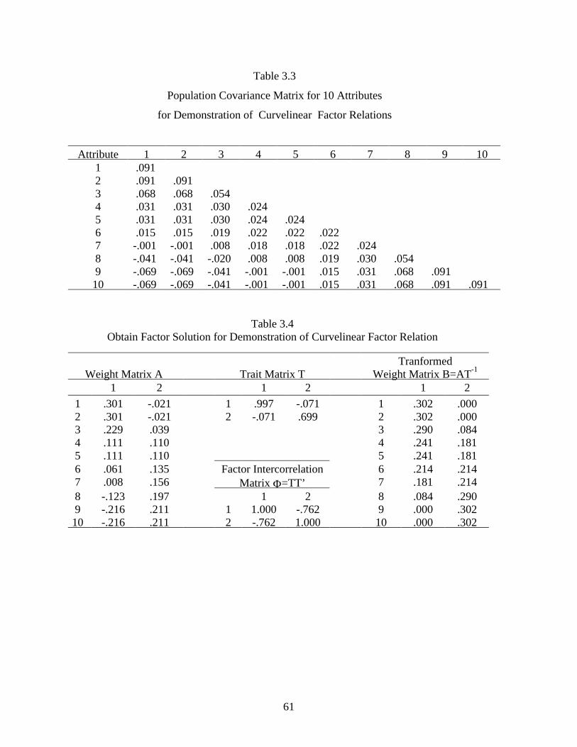
61

Table 3.3

Population Covariance Matrix for 10 Attributes

for Demonstration of Curvelinear Factor Relations

Attribute 1 2 3 4 5 6 7 8 9 101 .0912 .091 .0913 .068 .068 .0544 .031 .031 .030 .0245 .031 .031 .030 .024 .0246 .015 .015 .019 .022 .022 .0227 -.001 -.001 .008 .018 .018 .022 .0248 -.041 -.041 -.020 .008 .008 .019 .030 .0549 -.069 -.069 -.041 -.001 -.001 .015 .031 .068 .09110 -.069 -.069 -.041 -.001 -.001 .015 .031 .068 .091 .091

Table 3.4Obtain Factor Solution for Demonstration of Curvelinear Factor Relation

Weight Matrix A Trait Matrix TTranformed

Weight Matrix B=AT-1

1 2 1 2 1 2

1 .301 -.021 1 .997 -.071 1 .302 .0002 .301 -.021 2 -.071 .699 2 .302 .0003 .229 .039 3 .290 .0844 .111 .110 4 .241 .1815 .111 .110 5 .241 .1816 .061 .135 Factor Intercorrelation 6 .214 .2147 .008 .156 Matrix Φ=TT’ 7 .181 .2148 -.123 .197 1 2 8 .084 .2909 -.216 .211 1 1.000 -.762 9 .000 .30210 -.216 .211 2 -.762 1.000 10 .000 .302

62

permissible values (e.g., 0 and 1). Thus, the view that a binary surface attribute is a measure of an

underlying continuous factor implies that the relationship of the attribute to the factor must be

curvelinear.

To demonstrate the effects of such relationships, an artificial population covariance

matrix was constructed for 10 binary items. The items were defined as varying in difficulty,

where difficulty is defined as the proportion of the population which provides the correct

response to the item. Thus, lower values of this index represent more difficult items. Item

difficulties for the ten items are shown in Table 3.5. Each of these items was considered to be a

measure of a single common factor. Thus, the theoretical weights for the factor on the items were

all unity. This implies that the theoretical correlations among these 10 items would all be unity.

Given that these items would form a perfect Guttman scale (i.e., if an individual produces the

correct response to a given item, the individual will also produce the correct response to all easier

items), it is possible to obtain the actual population correlation matrix for the items. This matrix,

shown in Table 3.5, contains phi-coefficients representing the actual relationship for each pair of

binary items.

The correlation matrix in Table 3.5 represents a standardized version of a covariance

matrix for surface attributes. Factor analysis procedures were applied to this matrix toDCC

determine whether a solution could be obtained which fit the covariances among these items

perfectly. Despite the fact that the items are defined as being measures of a single factor, a

one-factor solution does not provide perfect fit to . In fact, could not be fit perfectlyD DCC CC

using any small number of factors. For illustrative purposes, a two-factor orthogonal solution is

shown in Table 3.6. This solution fits fairly well; that is, the elements of the resulting matrix?D

are not large. However, the important point is that it does not fit perfectly. The reason for this is

that the linear model cannot account for the relationships represented in because theseDCC

relationships arise from an underlying structure where the effects of the factors on the surface

attributes are curvelinear.

It is interesting to note the pattern of weights found in the solution shown in Table 3.6.

Factor 1 seems to differentiate items of medium difficulty from items of extreme difficulty (i.e.,

either very difficult or very easy). Factor 2 shows a continuum of weights from low to high

according to the difficulty of the items. Such factors are routinely observed when factor

analyzing binary data in practice, and have often been called "difficulty factors". For some time

they have been thought to be artifacts related to the presence of items of varying difficulty

(Gourlay, 1951; Guilford, 1941; Wherry & Gaylord, 1951).. However, they have been

recognized more recently as arising from non-linearities in the relationships of the items to the

factors (Gibson, 1959, 1960; McDonald, 1965a). The general point to recognize is that when

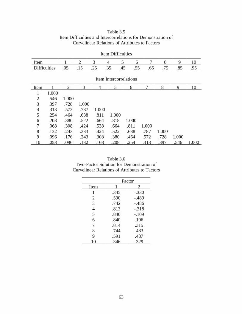
63

Table 3.5Item Difficulties and Intercorrelations for Demonstration of

Curvelinear Relations of Attributes to Factors

Item Difficulties

Item 1 2 3 4 5 6 7 8 9 10Difficulties .05 .15 .25 .35 .45 .55 .65 .75 .85 .95

Item Intercorrelations

Item 1 2 3 4 5 6 7 8 9 101 1.0002 .546 1.0003 .397 .728 1.0004 .313 .572 .787 1.0005 .254 .464 .638 .811 1.0006 .208 .380 .522 .664 .818 1.0007 .068 .308 .424 .538 .664 .811 1.0008 .132 .243 .333 .424 .522 .638 .787 1.0009 .096 .176 .243 .308 .380 .464 .572 .728 1.00010 .053 .096 .132 .168 .208 .254 .313 .397 .546 1.000

Table 3.6Two-Factor Solution for Demonstration of

Curvelinear Relations of Attributes to Tactors

FactorItem 1 2

1 .345 -.3302 .590 -.4893 .742 -.4864 .813 -.3185 .840 -.1096 .840 .1067 .814 .3158 .744 .4839 .591 .48710 .346 .329

64

there exist curvelinear relations of attributes to factors, the linear factor model is not appropriate.

If used, it will yield artifactual factors arising from non-linearities in the relations of attributes to

factors.

To summarize the issue of linearity in the common factor model, it should be understood

that the model assumes that the relations of the attributes to the factors are linear, but allows for

non-linear relations of attributes to each other, or of factors to each other. The model can be used

effectively when non-linear relations exist among attributes or among factors, as long as

relations of the attributes to the factors are linear. Of course, in the real world the relations of the

attributes to the factors in a given domain almost surely would not be exactly linear. It is likely

that such relations would be at least slightly nonlinear in many cases. However, as long as these

relations are approximately linear, the linear common factor model generally would provide an

adequate and useful representation of the relations. But when the relations of the attributes to the

factors are severely nonlinear, problems arise in the use of the model. As a result of the

recognition of this phenomenon, non-linear varieties of factor analysis have been developed (e.g.,

McDonald, 1967). However, such developments are beyond the scope of the present text, which

focuses on the linear common factor model.