CHAPTER 3

METHODOLOGY

3.1 Project Methodology

In the first stage, the theoretical analysis has been done to the WDM system such as

function of this system, the advantages, problem or the disadvantages and how the

development can be done.

In the second stage, after the achievement of the entire materials, simulator is used

to study the performance of the WDM systems. Optisys software has been used to

accomplish this work. A software simulation is important since it normally considers all

practical factors which may be too general to be considered in the theoretical development.

The design parameters are the system parameters that a designer can vary or

change in order to study their effect on the system’s performance. The design parameters

used are distance, bit rate, transmit power

In this project three performance parameters to evaluate the system under study. The

main parameter is bit error rate (BER). Received power or output power is the power that

is measured at the receiver and given in dBm.

3.2 Design Parameter

The design parameters are the system parameters that a designer can vary or

change in order to study their effect on the system’s performance. The design parameters

used are distance, bit rate, transmit and received power and chip spacing. Each of the

design parameters involved in this study are explained in the following subsections.

3.2.1 Distance

Lengthening the transmission distance is one of the main objectives of this project.

The effect of the length increment is explicated by the amount of dispersion and loss that

the signal experiences. The transmission distance is basically represented by the fiber

length. The distance of the fiber is characterized by the light propagation time, line

attenuation (loss), and dispersion.

3.2.2 Bit Rate

Bit rate is also known as data transfer rate (or data rate in short). Bit rate is the

number of bits that can be transmitted per second over a channel. It is usually measured in

bit per second (bps) and is different from the bandwidth that is measured in hertz. It is the

direct measure of information carrying capacity of a digital communications link or

network. The system bandwidth that is required to carry a signal may be more than or equal

to the bit rate. In this study four main bit rate 100 Mbps, 155 Mbps, 622 Mbps and 1Gbps

are used.

3.2.3 Transmission Power

Transmission power is measured in dBm. The need for enough light to overcome

all the optical transmission losses and to achieve desired BER is related to power. It must

be considered in a way to allow for system aging, fluctuation, repairs and not to overload

the receiver [18]. The coupling of the optical power from a source into a fiber needs the

consideration of the numerical aperture, core size, refractive index profile, and core-

cladding index difference of the fiber, plus the size, and angular power distribution of the

optical source.

3.2.4 Photodetector Types

Generally, there are many types of photodetectors for light detection and

conversion. PIN photodiode is the most common in the optical fiber telecommunication

systems. It has a wide intrinsic semiconductor layer between the P and N regions.

Another type of photodiode is the APD. It is popular used in the optical

telecommunication. Having internal gain, the APDs are much more sensitive than PIN

photodiodes.

Different system performance can be achieved by changing the photodiode at the

receiver. PIN and APD (avalanche photodiode) are the main types. Different device

characteristics, and different material profile used to construct such device might affect

the system performance significantly.

3.2.5 Wavelength Separation

Multi-wavelength transmission using one fiber is well known as wavelength

division multiplexing (WDM), and becomes a wide field. WDM can make both an

efficient use of the available transmission bandwidth provided by single mode optical

fibers, and also provide more flexibility in an optical network design.

3.3 Performance Parameter

The main parameter is bit error rate (BER). The other performance parameters that

used in this study are the received power or the output power and the noise power.

3.3.1 Bit Error Rate (BER)

BER is the probability of errors in number of bits of data over the total transmitted

bits at a certain time interval. Typically, error rate for optical communication system

ranges from 10-9 to 10-12 depending on the service types. In the simulator the BER is

measured by the eye diagram analyzer in the system layout.

3.3.2 Received Power (Output Power)

Received power or output power is the power that is measured at the receiver and

given in dBm. Note that it is the averaged total power which is considered, not the peak

power. In the experiment, the averaged total power is measured by using a power meter

while an Optical Spectrum Analyzer (OSA) is used for peak power.

3.3.3 Noise Power

Receiver noise is defined here as any signal power present in the receiver other than

the desired signal. This includes any unwanted disturbances that mask, corrupt, reduce the

information content of, or interfere with the desired signal.

3.3.4 Eye Pattern

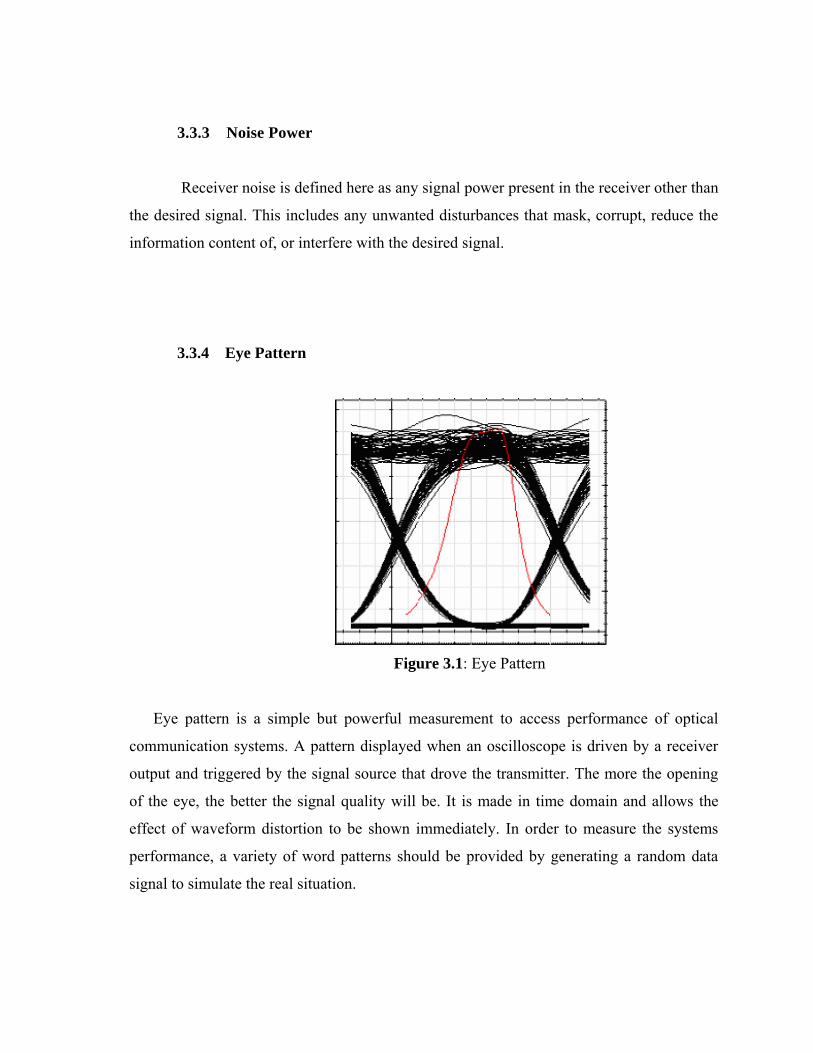
Figure 3.1: Eye Pattern

Eye pattern is a simple but powerful measurement to access performance of optical

communication systems. A pattern displayed when an oscilloscope is driven by a receiver

output and triggered by the signal source that drove the transmitter. The more the opening

of the eye, the better the signal quality will be. It is made in time domain and allows the

effect of waveform distortion to be shown immediately. In order to measure the systems

performance, a variety of word patterns should be provided by generating a random data

signal to simulate the real situation.

3.4 Simulation Analysis

Computer simulations are used particularly when analytical solutions are difficult or

impossible to formulate without excessive approximation [19], for example when modeling

the interaction of the dynamics of lasers with fibers [20], when studying statistical noise in

complex systems [21], when optimizing modulation format for long haul transmission [22],

when investigating dispersion and its composition [23], exploring nonlinear effects in fibers

[24-26] and when comparing fiber types [27].

In this research, parts of the study were carried out using simulation software,

Optical Communication System Design Software Version 5.0. This is recognized software,

which has been widely used and the results are being reported in reputable international

journal [28]. The extensive library of active and passive components includes realistic,

wavelength-dependent parameters. Parameter sweep function allows the user to investigate

the effect of particular device specifications on system performance.

OptiSystem is an innovative optical communication system simulation package that

designs, tests, and optimizes virtually any type of optical link in the physical layer of a

broad spectrum of optical networks, from analog video broadcasting systems to

intercontinental backbones.

OptiSystem is a stand-alone product that does not rely on other simulation

frameworks. It is a system level simulator based on the realistic modeling of fiber-optic

communication systems. It possesses a powerful new simulation environment and a truly

hierarchical definition of components and systems. Its capabilities can be extended easily

with the addition of user components, and can be seamlessly interfaced to a wide range of

tools.

3.4.1 OptiSystem To start OptiSystem, perform the following action.

Action

• From the Start menu, select Programs > Optiwave Software> OptiSystem 5 > OptiSystem.

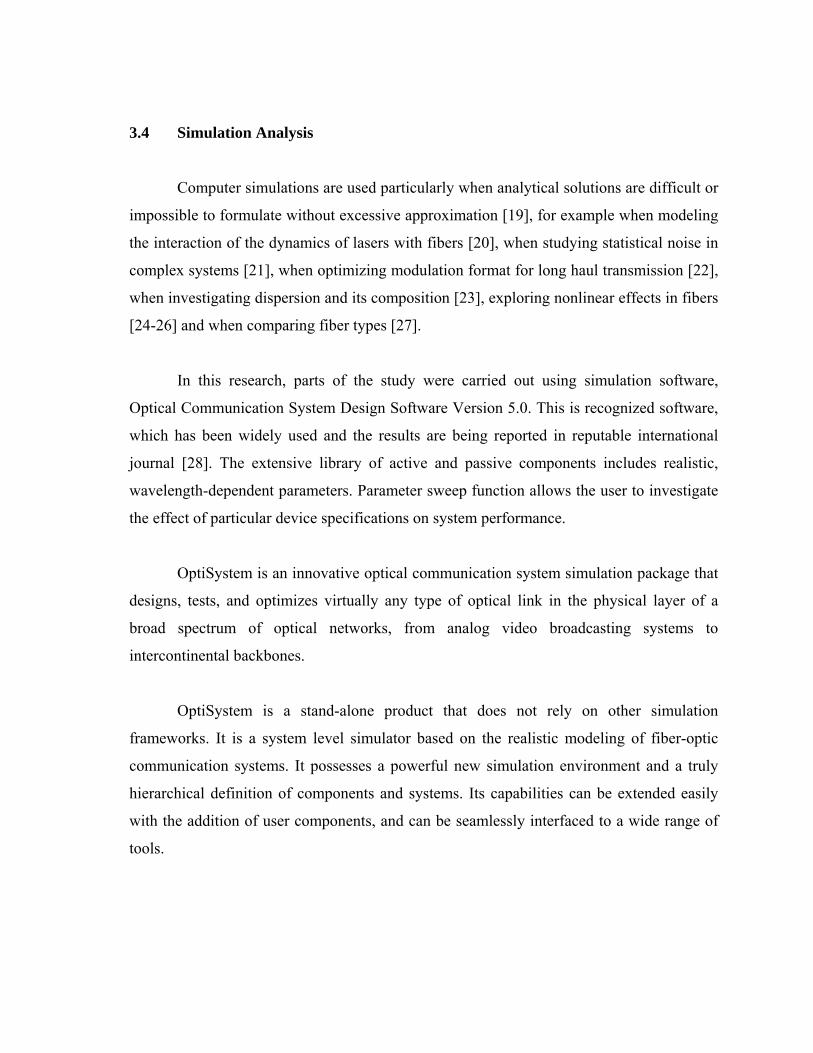
OptiSystem loads and the graphical user interface appear (see Figure 3.2).

Figure 3.2: OptiSystem graphical user interface (GUI)

Dockers

Use dockers, located in the main layout, to display information about the active (current)

project:

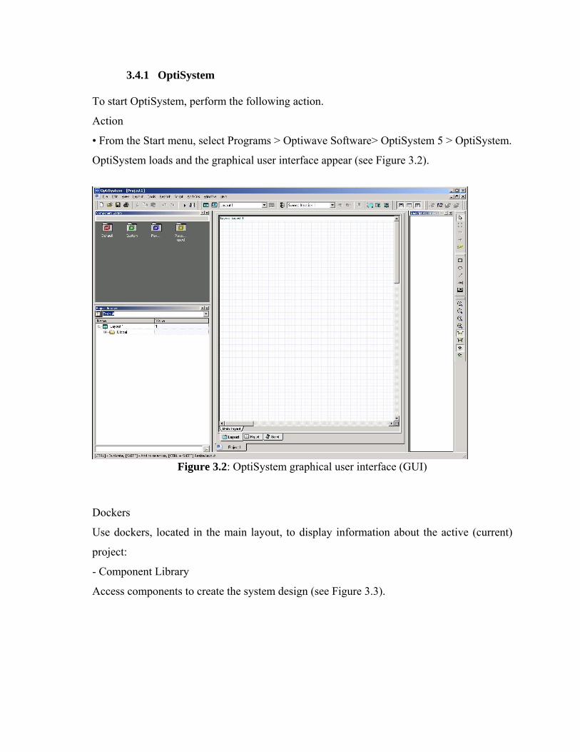
- Component Library

Access components to create the system design (see Figure 3.3).

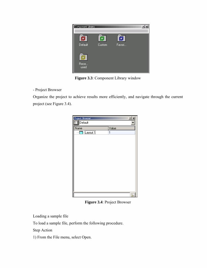
Figure 3.3: Component Library window

- Project Browser

Organize the project to achieve results more efficiently, and navigate through the current

project (see Figure 3.4).

Figure 3.4: Project Browser

Loading a sample file

To load a sample file, perform the following procedure.

Step Action

1) From the File menu, select Open.

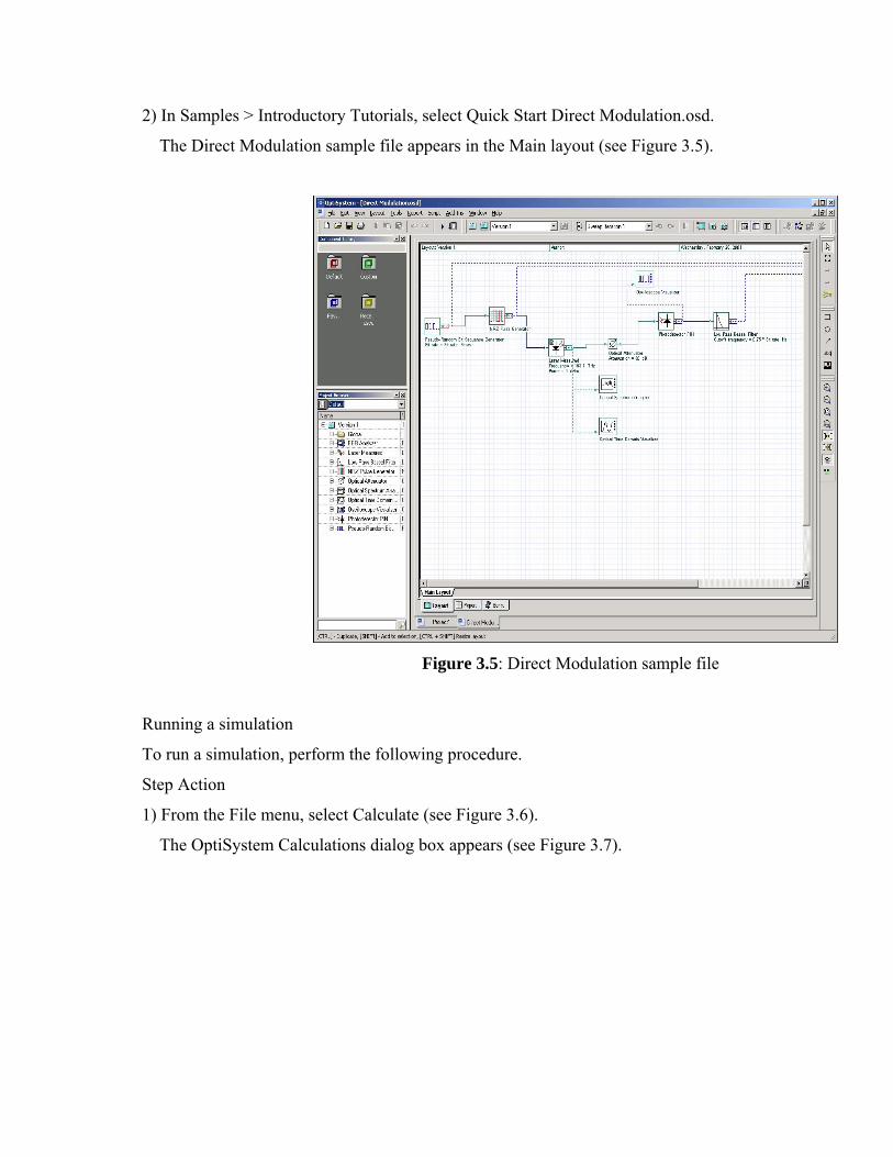
2) In Samples > Introductory Tutorials, select Quick Start Direct Modulation.osd.

The Direct Modulation sample file appears in the Main layout (see Figure 3.5).

Figure 3.5: Direct Modulation sample file

Running a simulation

To run a simulation, perform the following procedure.

Step Action

1) From the File menu, select Calculate (see Figure 3.6).

The OptiSystem Calculations dialog box appears (see Figure 3.7).

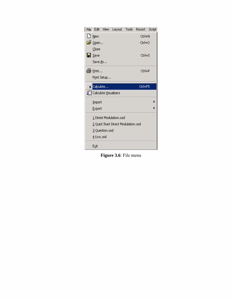
Figure 3.6: File menu

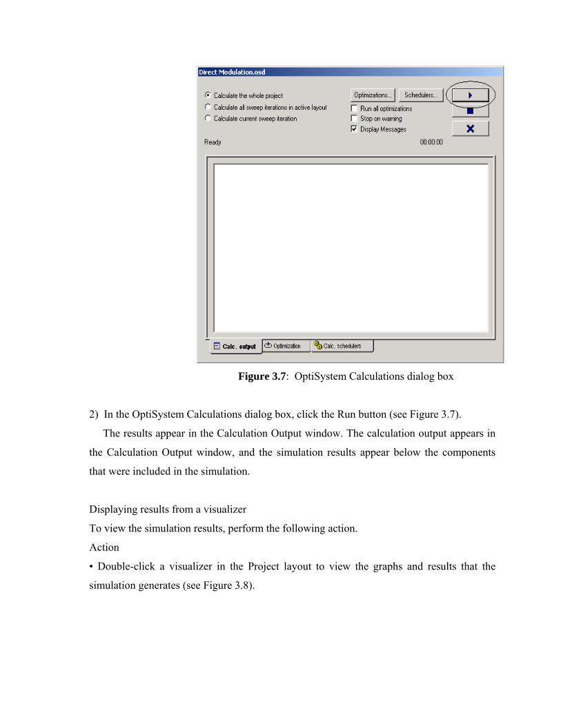
Figure 3.7: OptiSystem Calculations dialog box

2) In the OptiSystem Calculations dialog box, click the Run button (see Figure 3.7).

The results appear in the Calculation Output window. The calculation output appears in

the Calculation Output window, and the simulation results appear below the components

that were included in the simulation.

Displaying results from a visualizer

To view the simulation results, perform the following action.

Action

• Double-click a visualizer in the Project layout to view the graphs and results that the

simulation generates (see Figure 3.8).

Figure 3.8: Optical Time Domain Visualizer results