Embed Size (px)
Citation preview

Chapter 3
Load and Stress Analysis
September 28, 2013 Dr. Mohammad Suliman Abuhaiba, PE 1
Shear Force and Bending
Moments in Beams
Dr. Mohammad Suliman Abuhaiba, PE
September 28, 2013 2
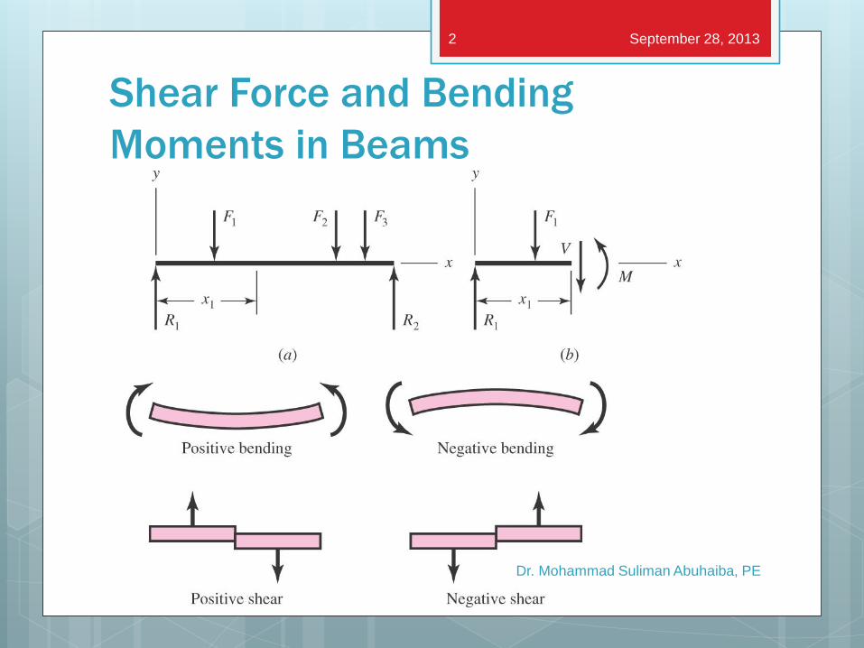
Change in shear force from A to B = area of load diagram between xA &
xB.
Change in moment from A to B = area of shear-force diagram between
xA & xB.
Distributed Load on Beam
Distributed load q(x):
load intensity
Dr. Mohammad Suliman Abuhaiba, PE
September 28, 2013 3
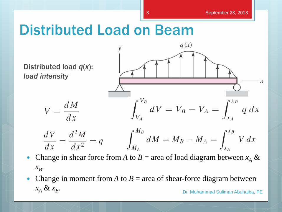
Shear-
Moment
Diagrams
Dr. Mohammad Suliman Abuhaiba, PE
Fig. 3−5
September 28, 2013 4
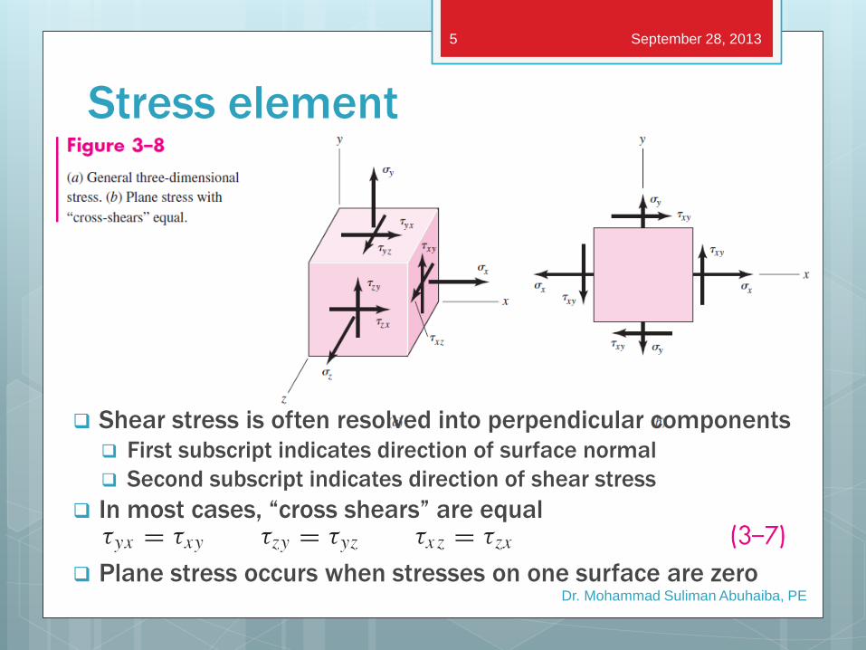
Stress element
Dr. Mohammad Suliman Abuhaiba, PE
September 28, 2013 5
Shear stress is often resolved into perpendicular components
First subscript indicates direction of surface normal
Second subscript indicates direction of shear stress
In most cases, “cross shears” are equal
Plane stress occurs when stresses on one surface are zero
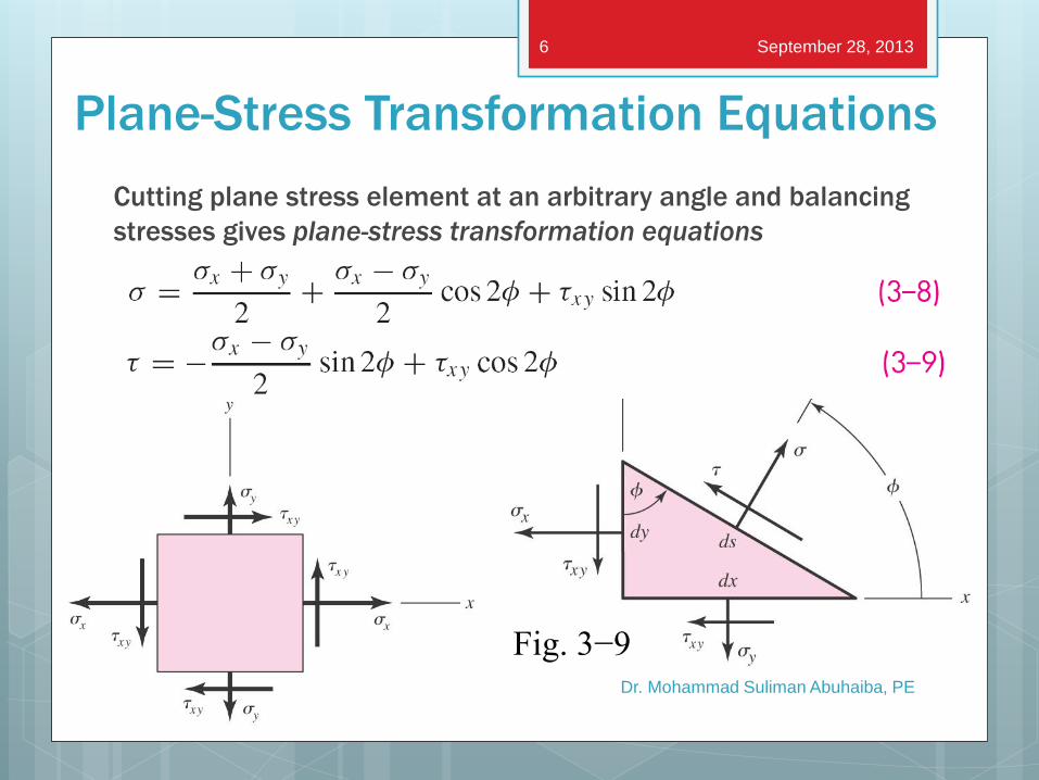
Plane-Stress Transformation Equations
Cutting plane stress element at an arbitrary angle and balancing
stresses gives plane-stress transformation equations
Dr. Mohammad Suliman Abuhaiba, PE
Fig. 3−9
September 28, 2013 6
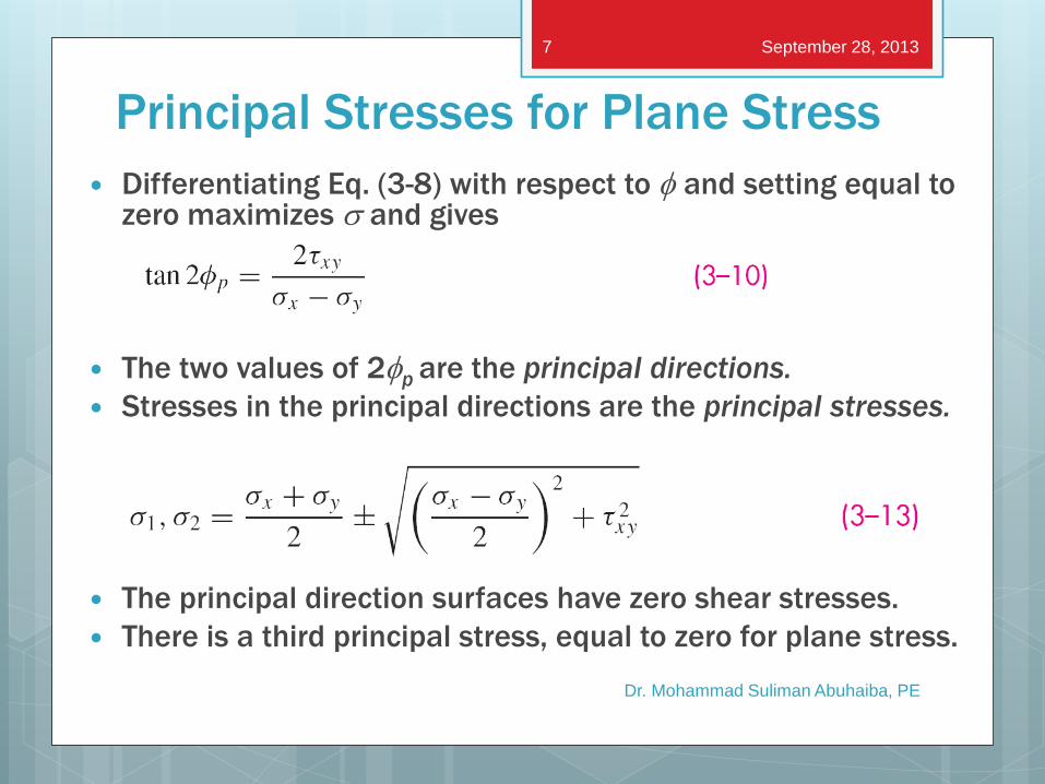
Principal Stresses for Plane Stress
Differentiating Eq. (3-8) with respect to f and setting equal to zero maximizes s and gives
The two values of 2fp are the principal directions.
Stresses in the principal directions are the principal stresses.
The principal direction surfaces have zero shear stresses.
There is a third principal stress, equal to zero for plane stress.
Dr. Mohammad Suliman Abuhaiba, PE
September 28, 2013 7
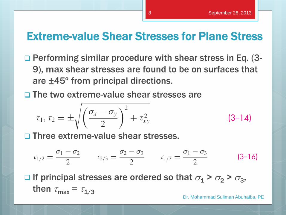
Extreme-value Shear Stresses for Plane Stress
Performing similar procedure with shear stress in Eq. (3-
9), max shear stresses are found to be on surfaces that
are ±45º from principal directions.
The two extreme-value shear stresses are
Three extreme-value shear stresses.
If principal stresses are ordered so that s1 > s2 > s3,
then tmax = t1/3
Dr. Mohammad Suliman Abuhaiba, PE
September 28, 2013 8
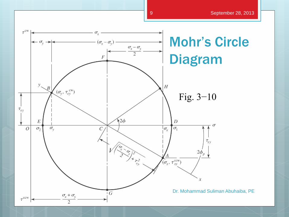
Mohr’s Circle
Diagram
Dr. Mohammad Suliman Abuhaiba, PE
Fig. 3−10
September 28, 2013 9
Dr. Mohammad Suliman Abuhaiba, PE
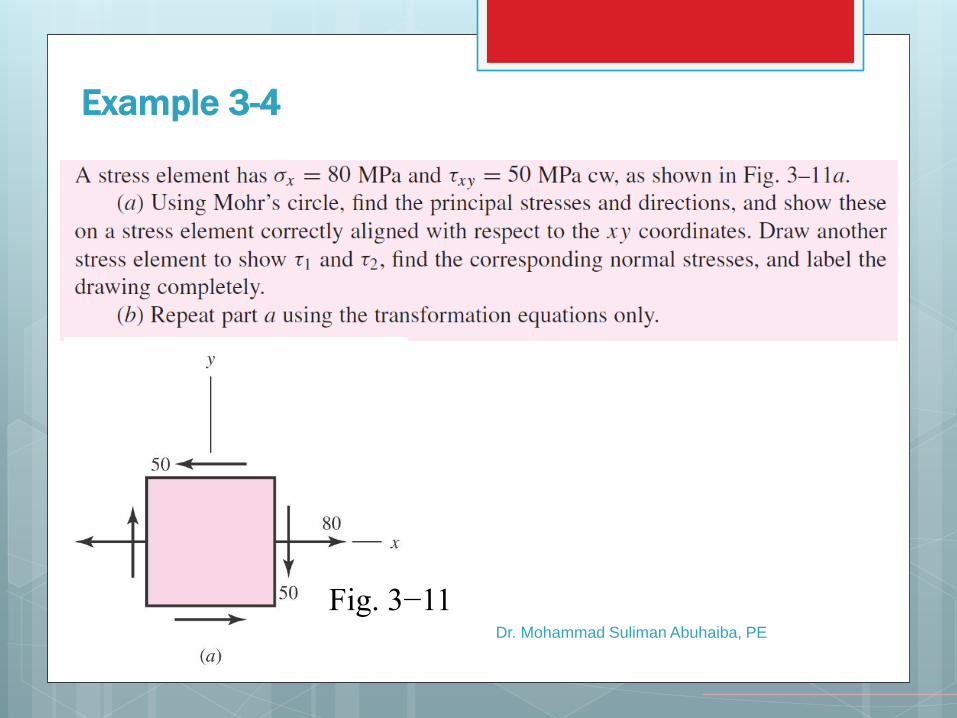
Example 3-4
Fig. 3−11
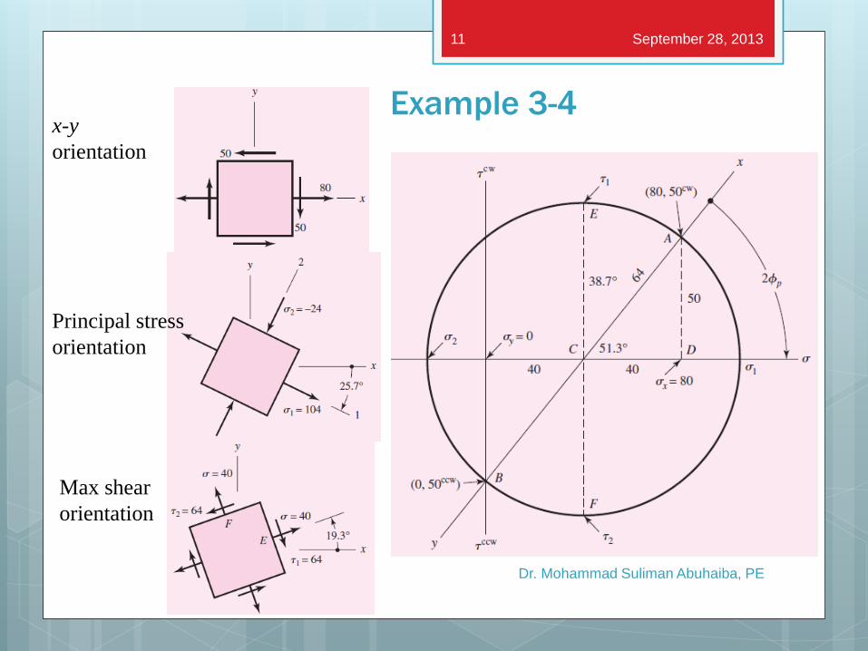
x-y
orientation
Principal stress
orientation
Max shear
orientation
September 28, 2013
Dr. Mohammad Suliman Abuhaiba, PE
11
Example 3-4
Example 3-4
Dr. Mohammad Suliman Abuhaiba, PE
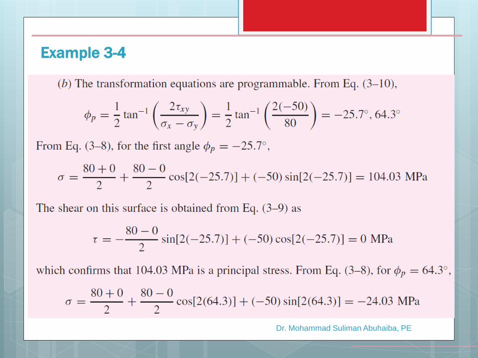
Example 3-4
Dr. Mohammad Suliman Abuhaiba, PE
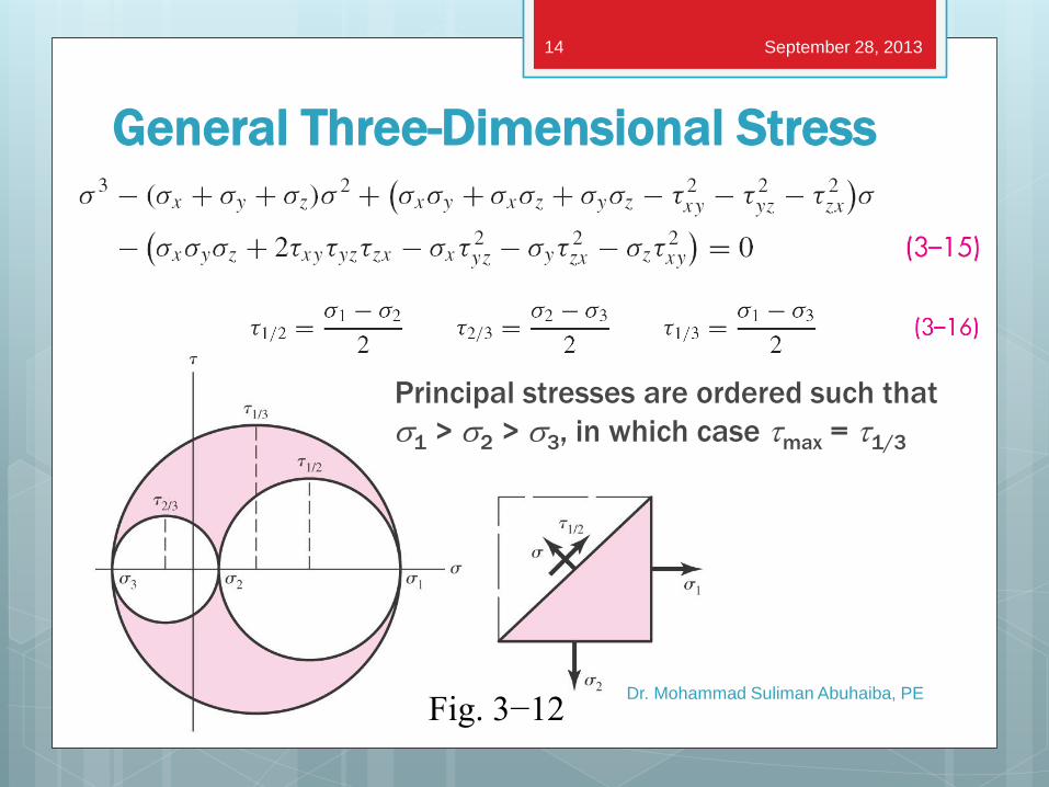
General Three-Dimensional Stress
Dr. Mohammad Suliman Abuhaiba, PE
Fig. 3−12
September 28, 2013 14
Principal stresses are ordered such that
s1 > s2 > s3, in which case tmax = t1/3
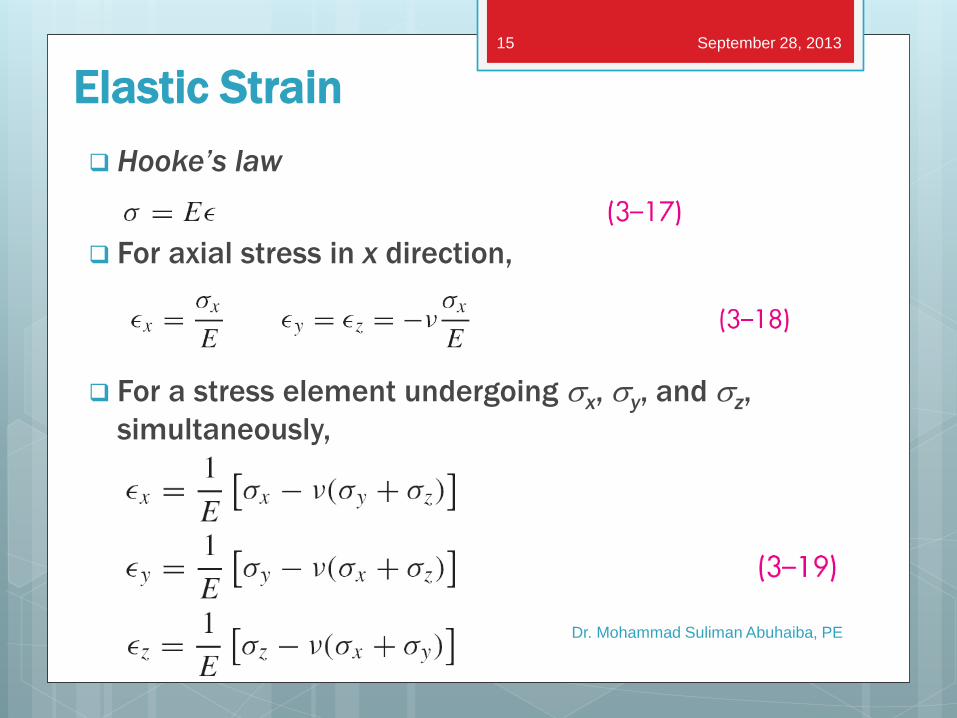
Hooke’s law
For axial stress in x direction,
For a stress element undergoing sx, sy, and sz,
simultaneously,
Elastic Strain
Dr. Mohammad Suliman Abuhaiba, PE
September 28, 2013 15
Elastic Strain
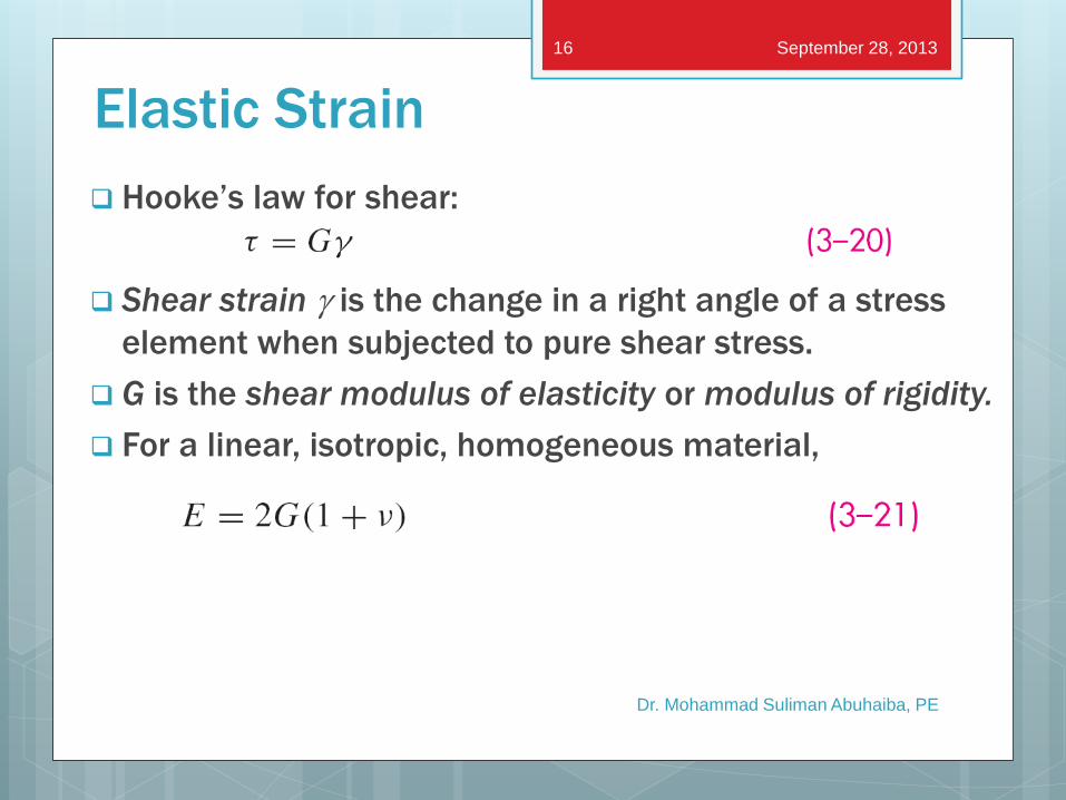
Hooke’s law for shear:
Shear strain g is the change in a right angle of a stress
element when subjected to pure shear stress.
G is the shear modulus of elasticity or modulus of rigidity.
For a linear, isotropic, homogeneous material,
Dr. Mohammad Suliman Abuhaiba, PE
September 28, 2013 16
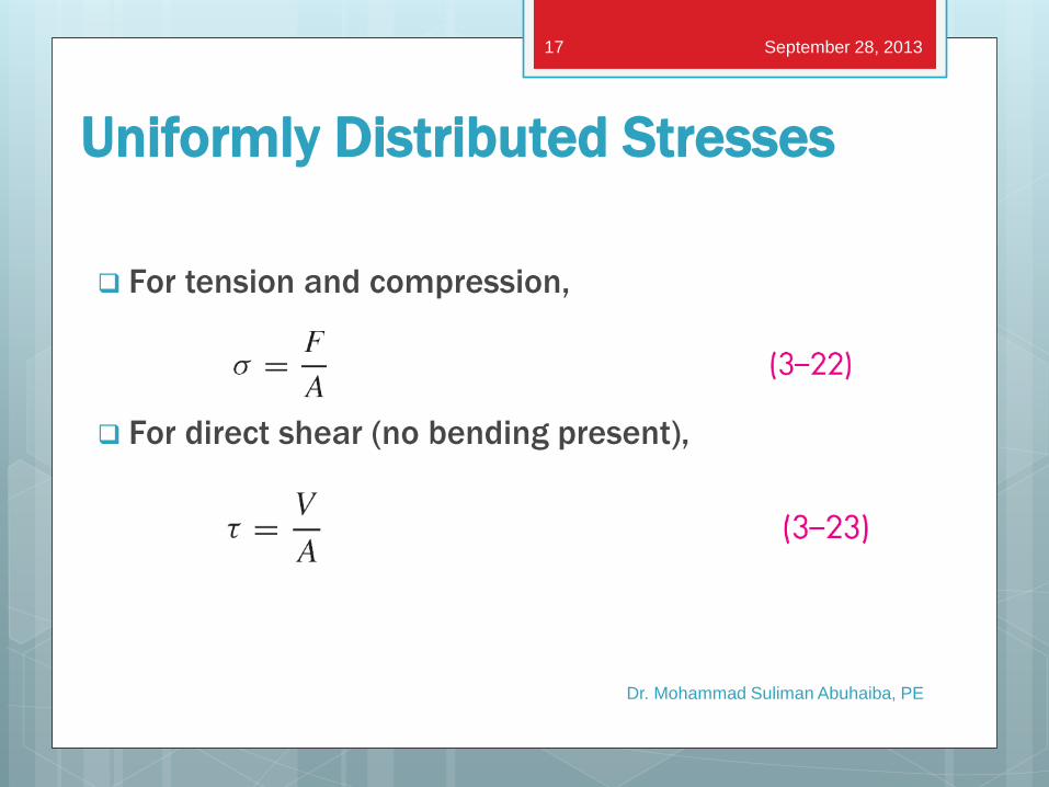
Uniformly Distributed Stresses
For tension and compression,
For direct shear (no bending present),
Dr. Mohammad Suliman Abuhaiba, PE
September 28, 2013 17
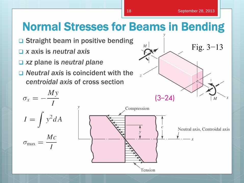
Normal Stresses for Beams in Bending Straight beam in positive bending
x axis is neutral axis
xz plane is neutral plane
Neutral axis is coincident with the
centroidal axis of cross section
Dr. Mohammad Suliman Abuhaiba, PE
Fig. 3−13
September 28, 2013 18
Dr. Mohammad Suliman Abuhaiba, PE
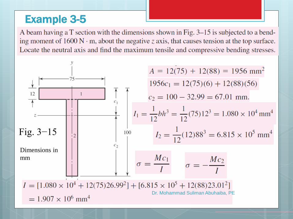
Example 3-5
Dimensions in
mm
Fig. 3−15
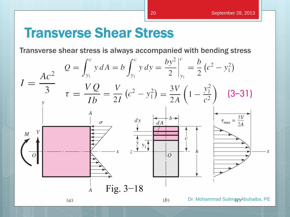
Transverse Shear Stress Transverse shear stress is always accompanied with bending stress
Dr. Mohammad Suliman Abuhaiba, PE
Fig. 3−18
September 28, 2013 20
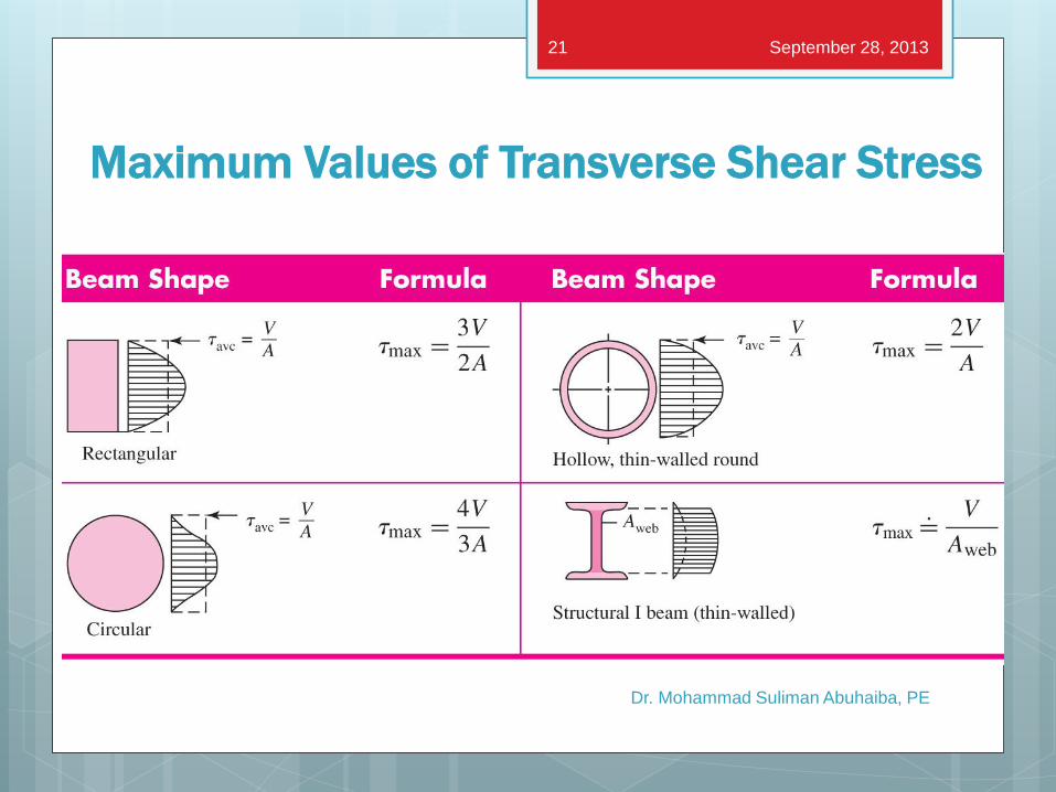
Maximum Values of Transverse Shear Stress
Dr. Mohammad Suliman Abuhaiba, PE
September 28, 2013 21
Dr. Mohammad Suliman Abuhaiba, PE
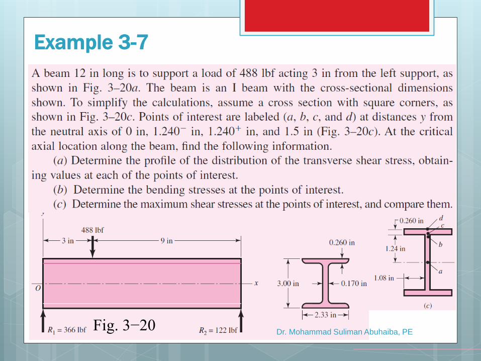
Example 3-7
Fig. 3−20
Dr. Mohammad Suliman Abuhaiba, PE
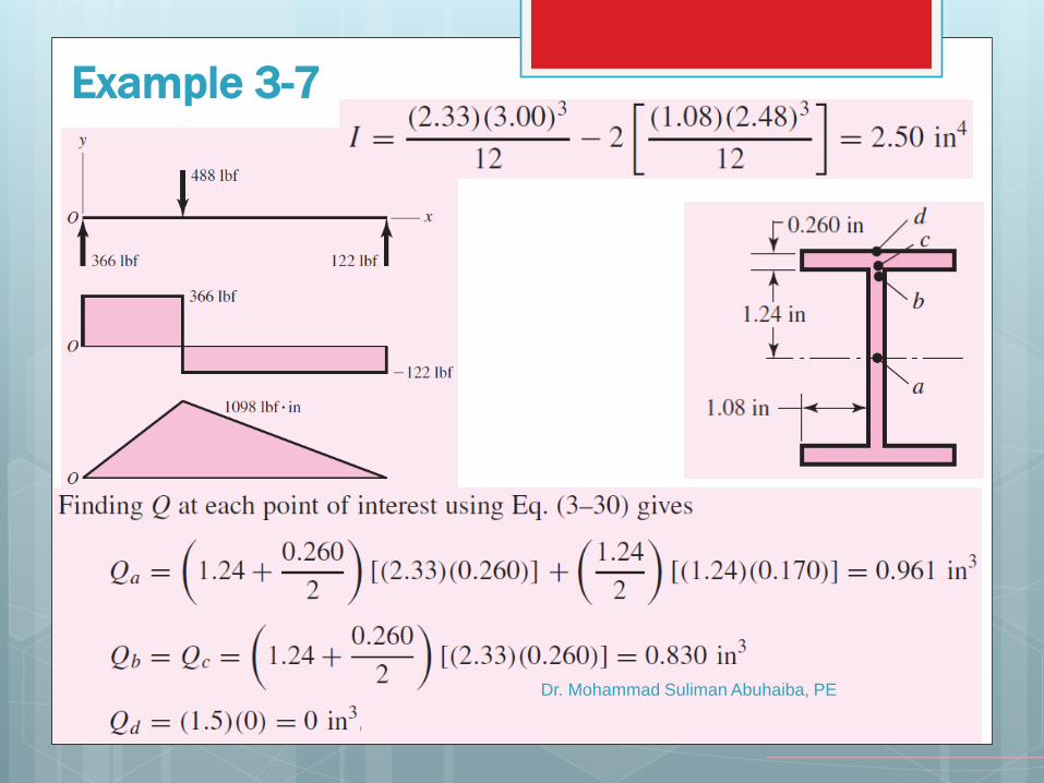
Example 3-7
Dr. Mohammad Suliman Abuhaiba, PE
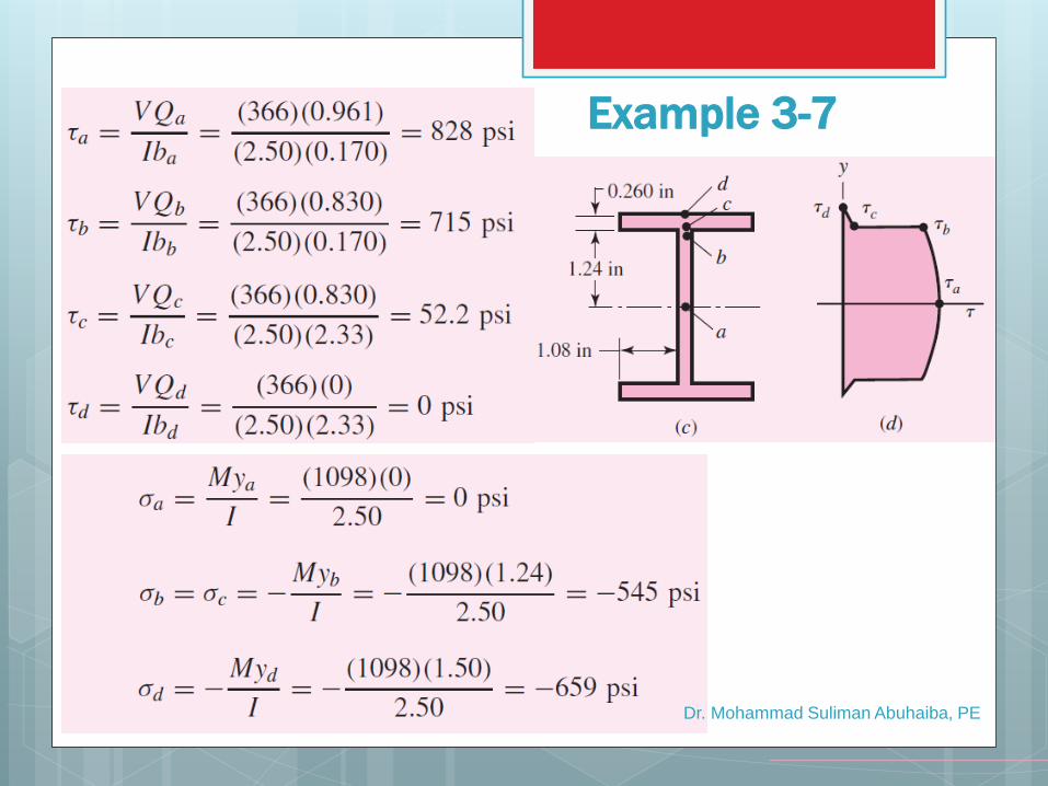
Example 3-7
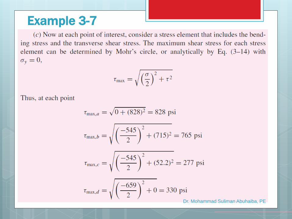
Dr. Mohammad Suliman Abuhaiba, PE
Example 3-7
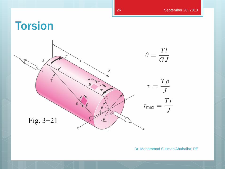
Torsion
Dr. Mohammad Suliman Abuhaiba, PE
Fig. 3−21
September 28, 2013 26
Dr. Mohammad Suliman Abuhaiba, PE
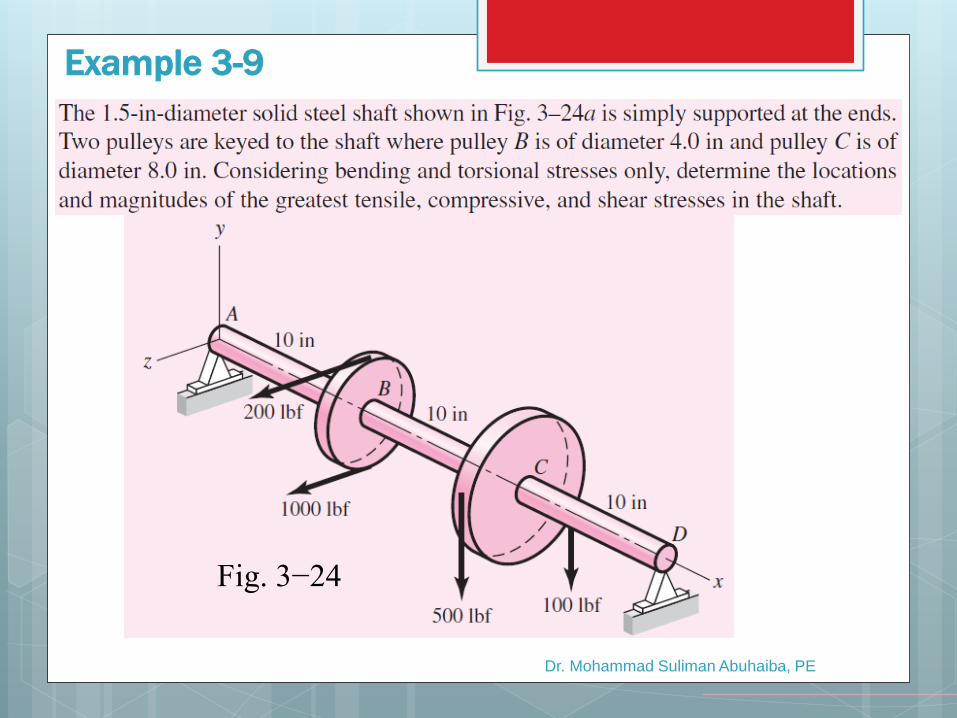
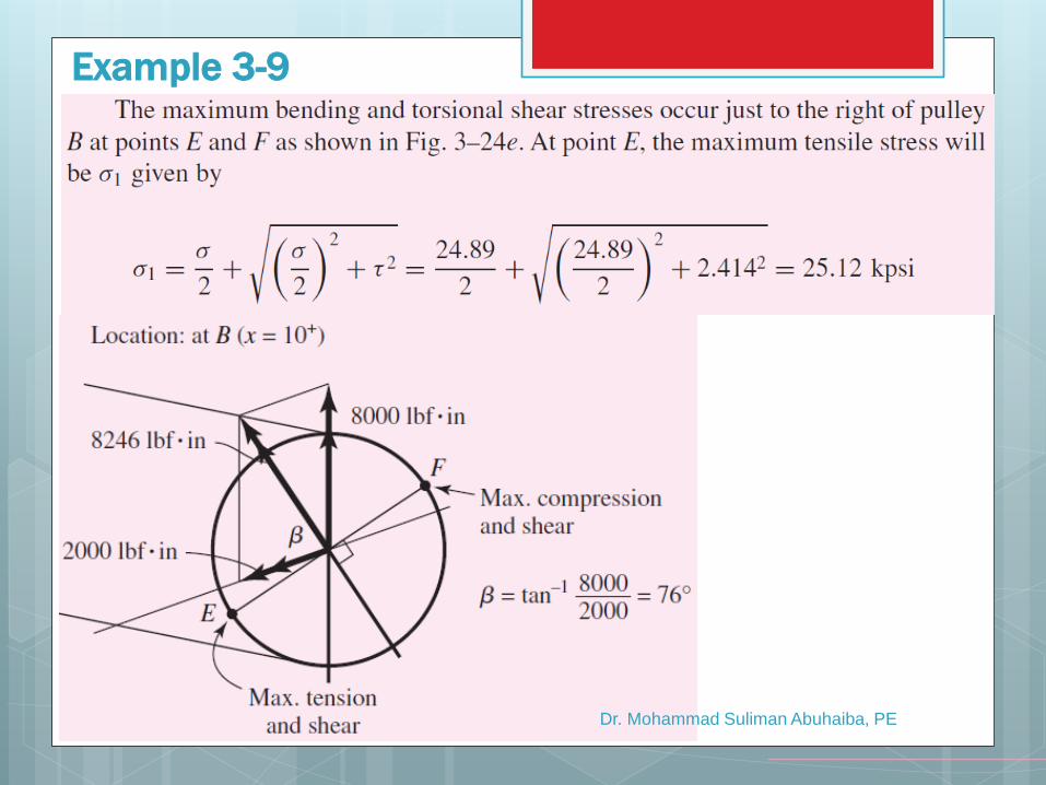
Example 3-9
Fig. 3−24
Dr. Mohammad Suliman Abuhaiba, PE
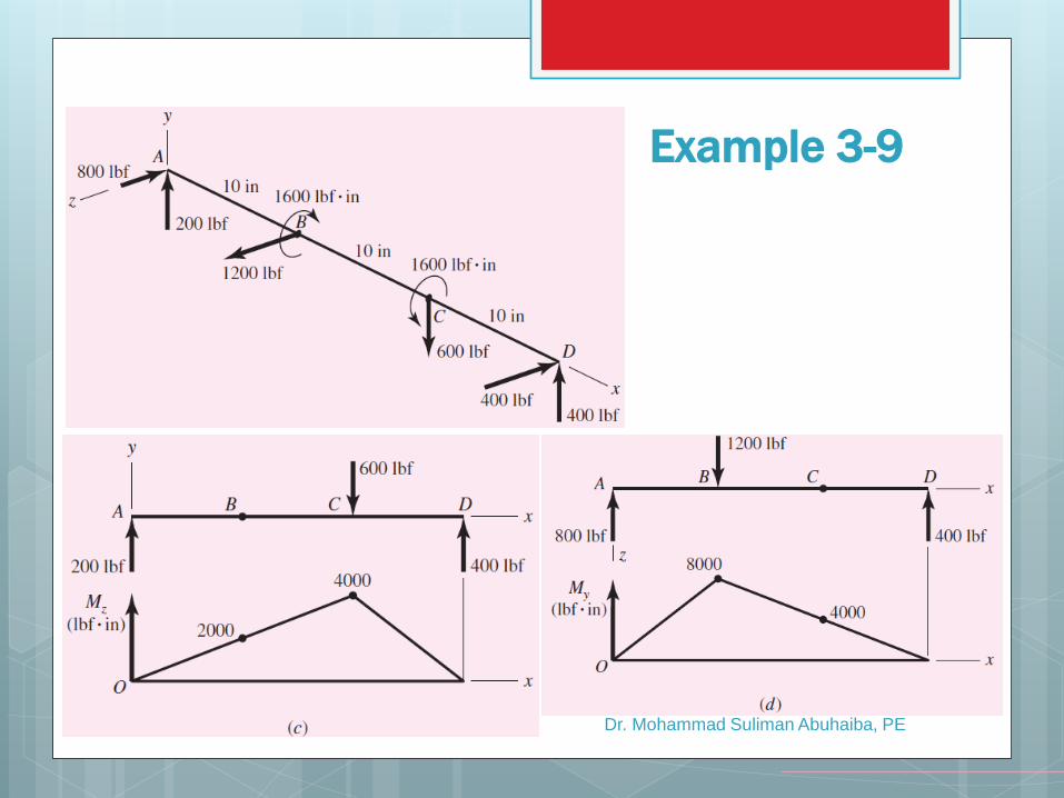
Example 3-9
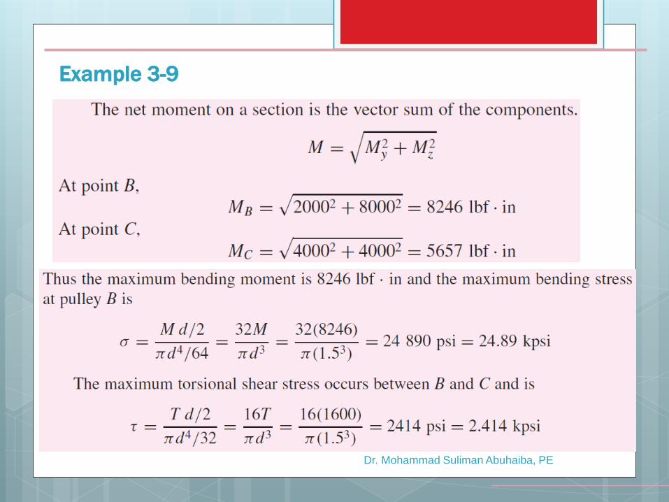
Example 3-9
Dr. Mohammad Suliman Abuhaiba, PE
Dr. Mohammad Suliman Abuhaiba, PE
Example 3-9
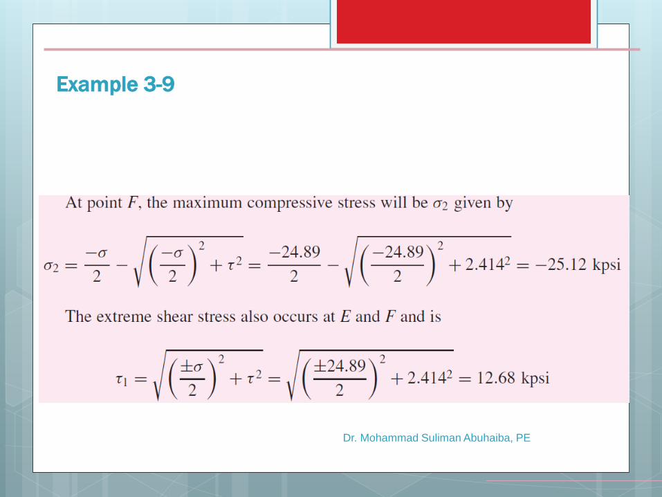
Example 3-9
Dr. Mohammad Suliman Abuhaiba, PE
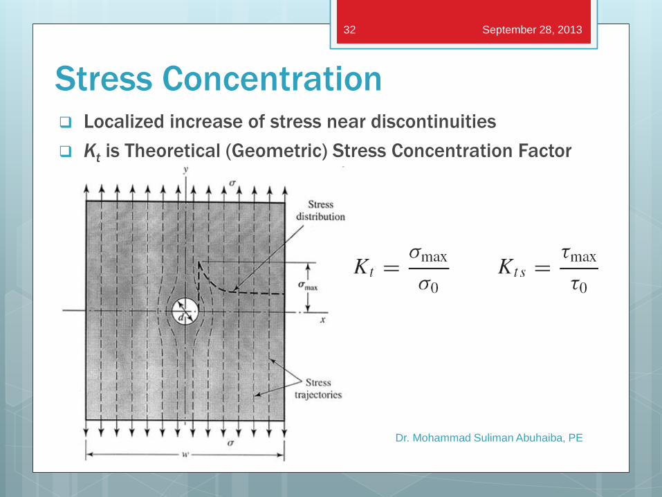
Stress Concentration Localized increase of stress near discontinuities
Kt is Theoretical (Geometric) Stress Concentration Factor
Dr. Mohammad Suliman Abuhaiba, PE
September 28, 2013 32
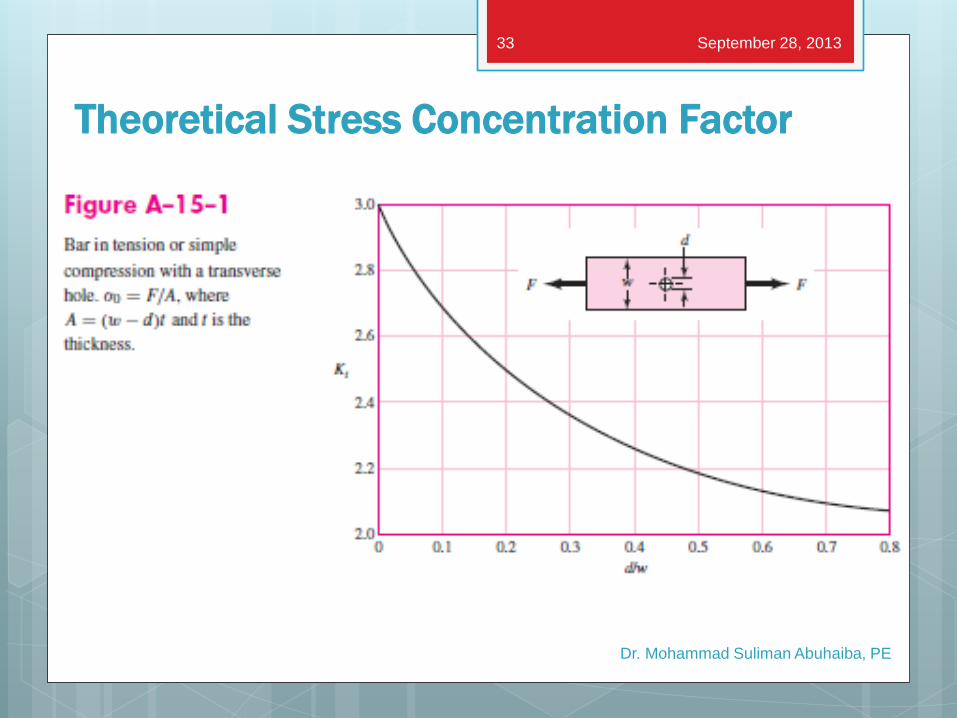
Theoretical Stress Concentration Factor
Dr. Mohammad Suliman Abuhaiba, PE
September 28, 2013 33
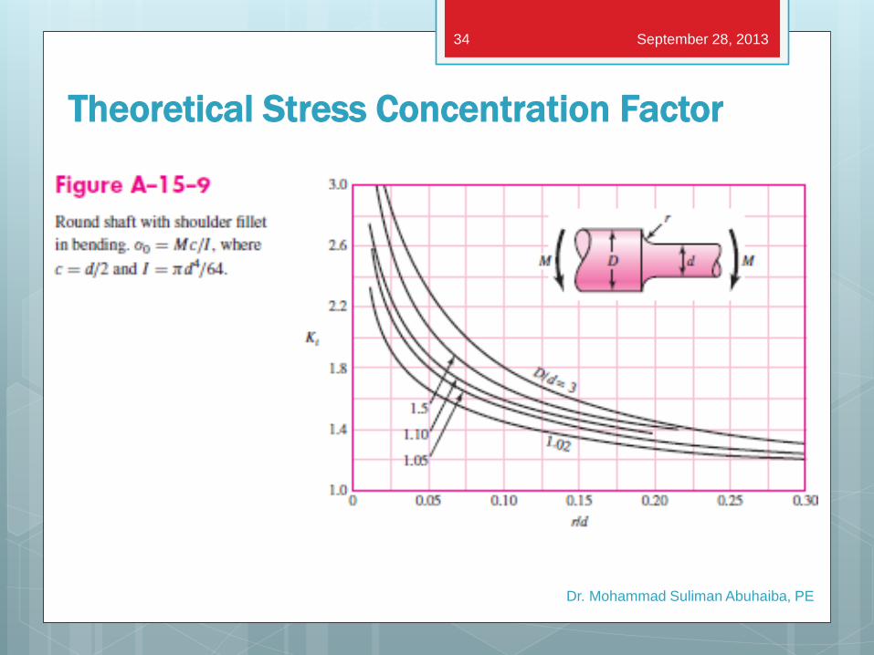
Theoretical Stress Concentration Factor
Dr. Mohammad Suliman Abuhaiba, PE
September 28, 2013 34
Stress Concentration for Static and
Ductile Conditions
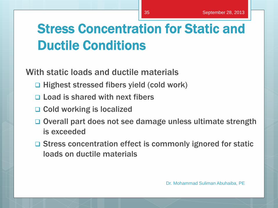
With static loads and ductile materials
Highest stressed fibers yield (cold work)
Load is shared with next fibers
Cold working is localized
Overall part does not see damage unless ultimate strength
is exceeded
Stress concentration effect is commonly ignored for static
loads on ductile materials
Dr. Mohammad Suliman Abuhaiba, PE
September 28, 2013 35
Dr. Mohammad Suliman Abuhaiba, PE
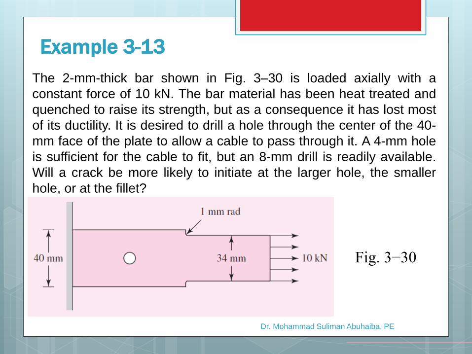
Example 3-13
Fig. 3−30
The 2-mm-thick bar shown in Fig. 3–30 is loaded axially with a
constant force of 10 kN. The bar material has been heat treated and
quenched to raise its strength, but as a consequence it has lost most
of its ductility. It is desired to drill a hole through the center of the 40-
mm face of the plate to allow a cable to pass through it. A 4-mm hole
is sufficient for the cable to fit, but an 8-mm drill is readily available.
Will a crack be more likely to initiate at the larger hole, the smaller
hole, or at the fillet?
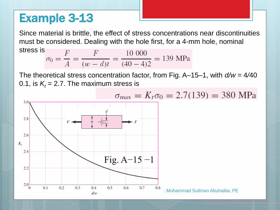
Since material is brittle, the effect of stress concentrations near discontinuities
must be considered. Dealing with the hole first, for a 4-mm hole, nominal
stress is
The theoretical stress concentration factor, from Fig. A–15–1, with d/w = 4/40
0.1, is Kt = 2.7. The maximum stress is
Dr. Mohammad Suliman Abuhaiba, PE
Example 3-13
Fig. A−15 −1
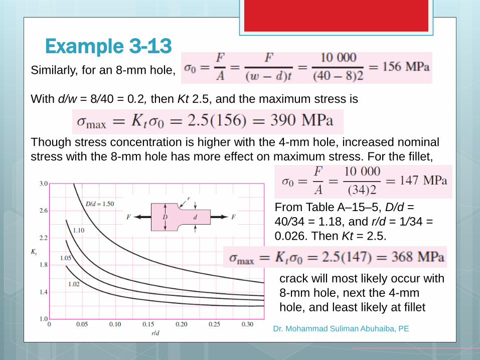
Similarly, for an 8-mm hole,
With d/w = 8/40 = 0.2, then Kt 2.5, and the maximum stress is
Though stress concentration is higher with the 4-mm hole, increased nominal
stress with the 8-mm hole has more effect on maximum stress. For the fillet,
Dr. Mohammad Suliman Abuhaiba, PE
Example 3-13
From Table A–15–5, D/d =
40/34 = 1.18, and r/d = 1/34 =
0.026. Then Kt = 2.5.
crack will most likely occur with
8-mm hole, next the 4-mm
hole, and least likely at fillet
Chapter 4
Deflection and Stiffness
September 28, 2013
Dr. Mohammad Suliman Abuhaiba, PE
39
Spring Rate
Relation between force and deflection, F = F(y)
Spring rate
For linear springs, k is constant, called spring constant
Dr. Mohammad Suliman Abuhaiba, PE
September 28, 2013 40
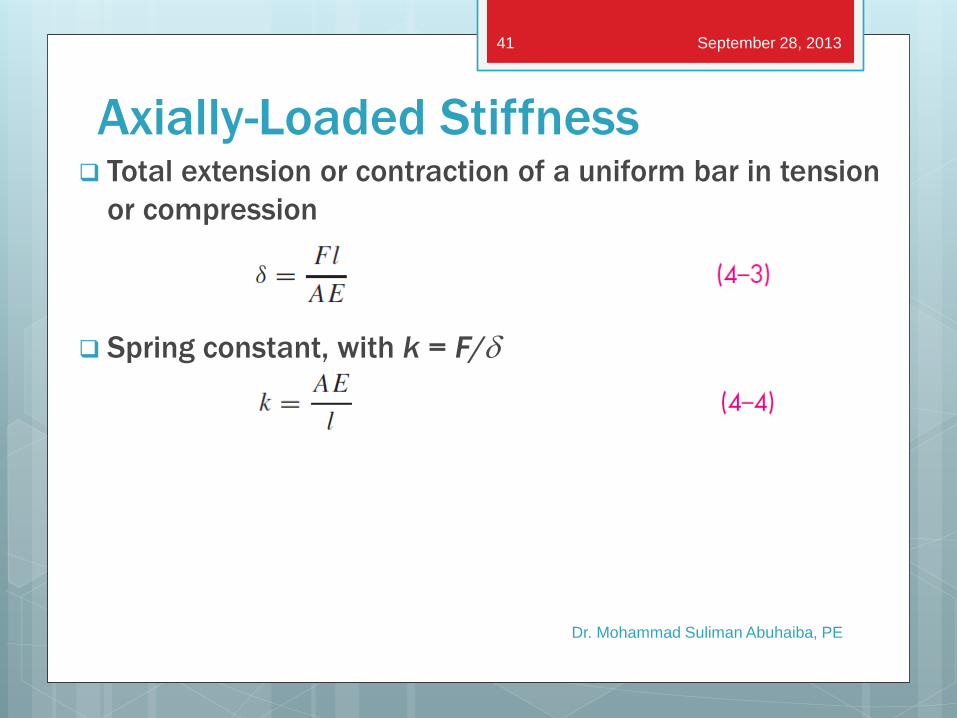
Axially-Loaded Stiffness Total extension or contraction of a uniform bar in tension
or compression
Spring constant, with k = F/d
Dr. Mohammad Suliman Abuhaiba, PE
September 28, 2013 41
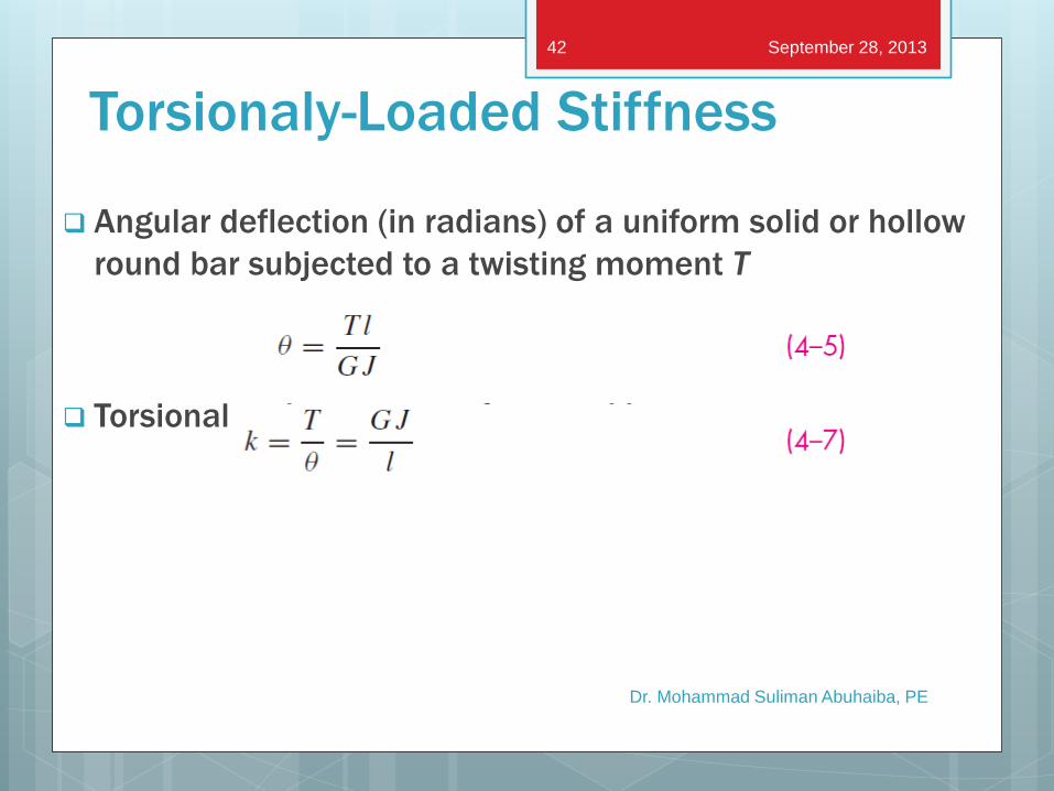
Torsionaly-Loaded Stiffness
Angular deflection (in radians) of a uniform solid or hollow
round bar subjected to a twisting moment T
Torsional spring constant for round bar
Dr. Mohammad Suliman Abuhaiba, PE
September 28, 2013 42
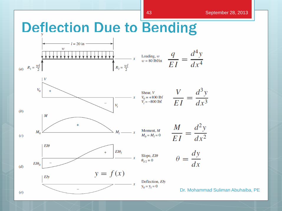
Deflection Due to Bending
Dr. Mohammad Suliman Abuhaiba, PE
September 28, 2013 43
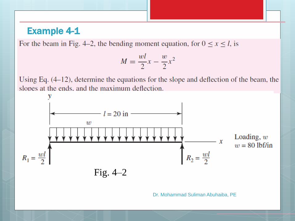
Example 4-1
Dr. Mohammad Suliman Abuhaiba, PE
Fig. 4–2
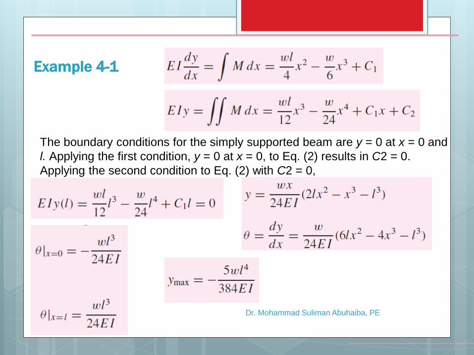
Example 4-1
Dr. Mohammad Suliman Abuhaiba, PE
The boundary conditions for the simply supported beam are y = 0 at x = 0 and
l. Applying the first condition, y = 0 at x = 0, to Eq. (2) results in C2 = 0.
Applying the second condition to Eq. (2) with C2 = 0,
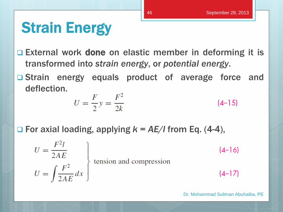
Strain Energy
External work done on elastic member in deforming it is
transformed into strain energy, or potential energy.
Strain energy equals product of average force and
deflection.
For axial loading, applying k = AE/l from Eq. (4-4),
Dr. Mohammad Suliman Abuhaiba, PE
September 28, 2013 46
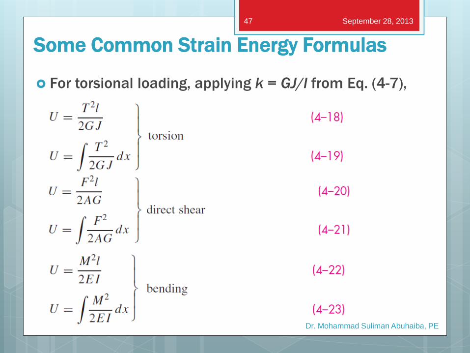
Some Common Strain Energy Formulas
For torsional loading, applying k = GJ/l from Eq. (4-7),
Dr. Mohammad Suliman Abuhaiba, PE
September 28, 2013 47
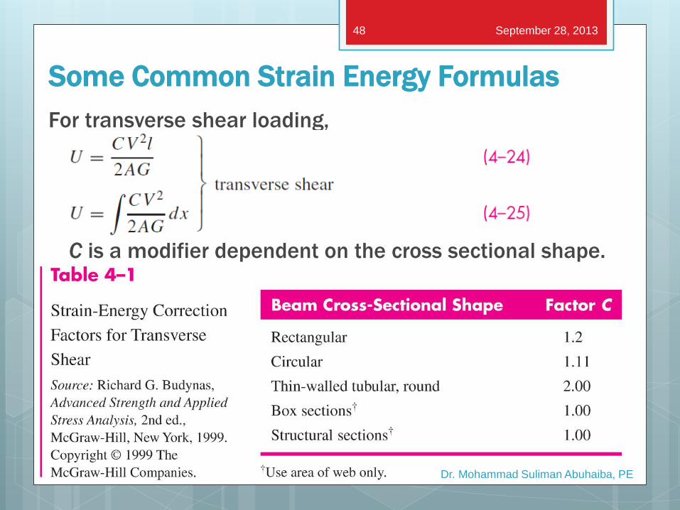
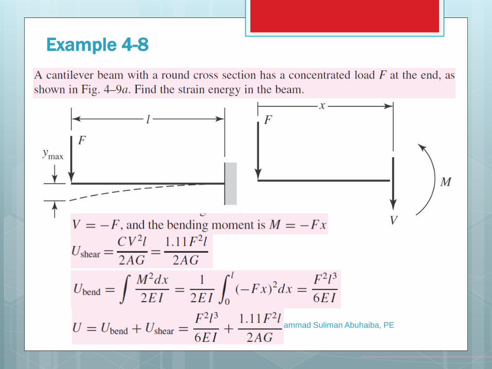
For transverse shear loading,
C is a modifier dependent on the cross sectional shape.
Dr. Mohammad Suliman Abuhaiba, PE
September 28, 2013 48
Some Common Strain Energy Formulas
Dr. Mohammad Suliman Abuhaiba, PE
Example 4-8
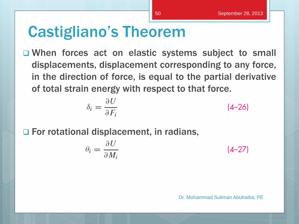
Castigliano’s Theorem
When forces act on elastic systems subject to small
displacements, displacement corresponding to any force,
in the direction of force, is equal to the partial derivative
of total strain energy with respect to that force.
For rotational displacement, in radians,
Dr. Mohammad Suliman Abuhaiba, PE
September 28, 2013 50
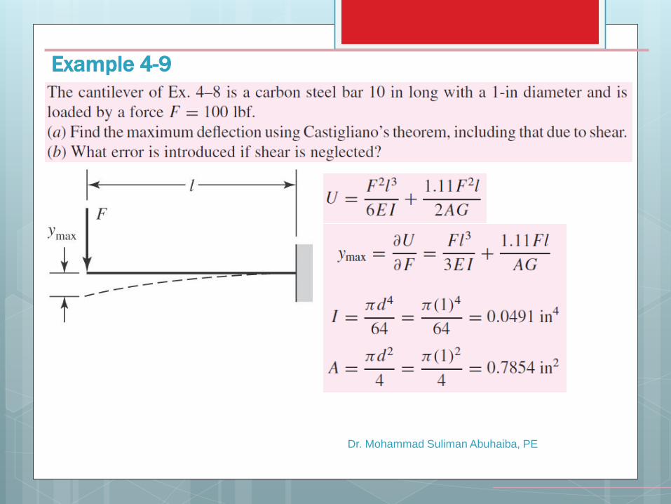
Example 4-9
Dr. Mohammad Suliman Abuhaiba, PE
Utilizing a Fictitious Force
Castigliano’s method can be used to find a deflection at a
point even if there is no force applied at that point.
Apply a fictitious force Q at the point, and in the direction,
of the desired deflection.
Set up the equation for total strain energy including
energy due to Q.
Take derivative of total strain energy with respect to Q.
Once derivative is taken, Q is no longer needed and can
be set to zero.
Dr. Mohammad Suliman Abuhaiba, PE
September 28, 2013 52
Dr. Mohammad Suliman Abuhaiba, PE
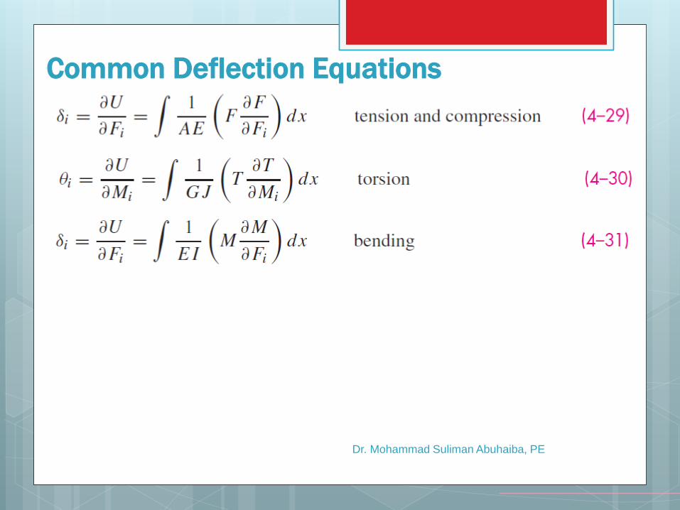
Common Deflection Equations
Dr. Mohammad Suliman Abuhaiba, PE
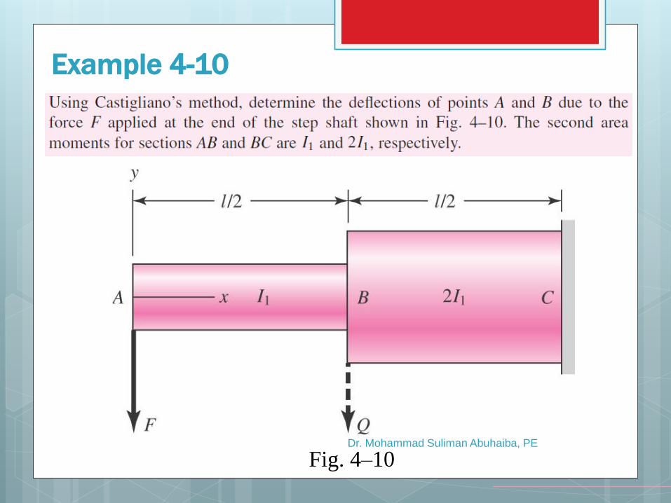
Example 4-10
Fig. 4–10
Dr. Mohammad Suliman Abuhaiba, PE
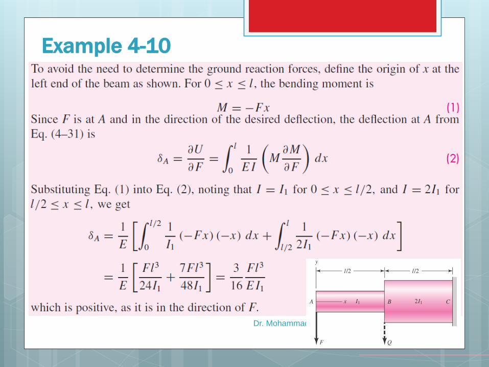
Example 4-10
Dr. Mohammad Suliman Abuhaiba, PE
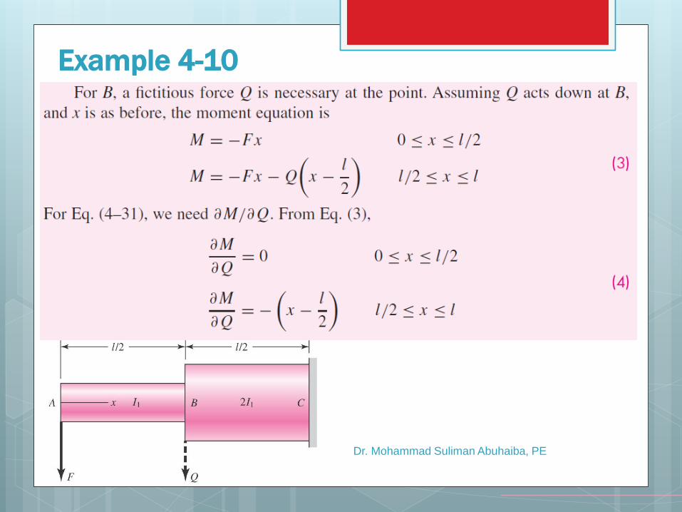
Example 4-10
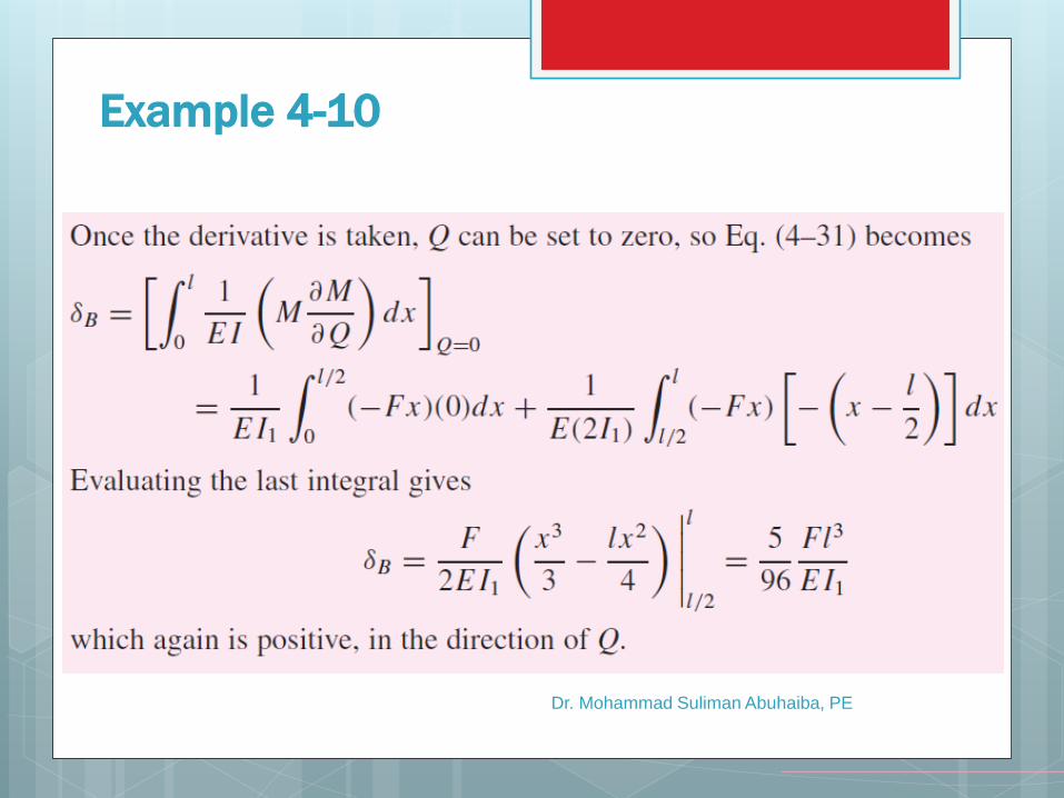
Dr. Mohammad Suliman Abuhaiba, PE
Example 4-10
Compression Members Column – A member loaded in compression such that
either its length or eccentric loading causes it to
experience more than pure compression
Four categories of columns
Long columns with central loading
Intermediate-length columns with central loading
Columns with eccentric loading
Struts or short columns with eccentric loading
Dr. Mohammad Suliman Abuhaiba, PE
September 28, 2013 58
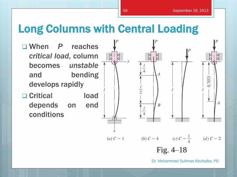
Long Columns with Central Loading
When P reaches
critical load, column
becomes unstable
and bending
develops rapidly
Critical load
depends on end
conditions
Dr. Mohammad Suliman Abuhaiba, PE
Fig. 4–18
September 28, 2013 59
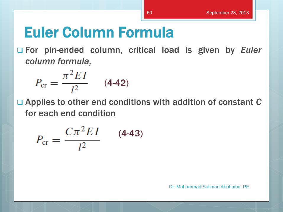
Euler Column Formula For pin-ended column, critical load is given by Euler
column formula,
Applies to other end conditions with addition of constant C
for each end condition
Dr. Mohammad Suliman Abuhaiba, PE
(4-42)
(4-43)
September 28, 2013 60
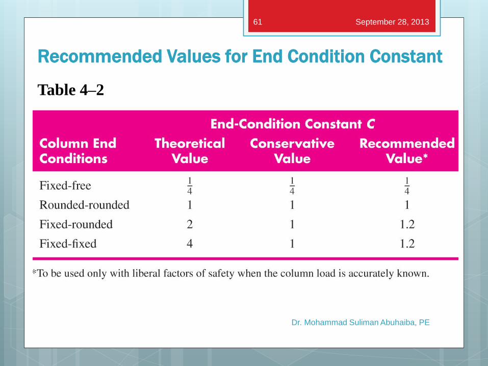
Recommended Values for End Condition Constant
Dr. Mohammad Suliman Abuhaiba, PE
Table 4–2
September 28, 2013 61
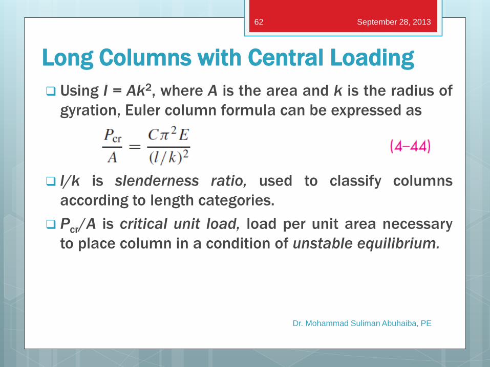
Long Columns with Central Loading
Using I = Ak2, where A is the area and k is the radius of
gyration, Euler column formula can be expressed as
l/k is slenderness ratio, used to classify columns
according to length categories.
Pcr/A is critical unit load, load per unit area necessary
to place column in a condition of unstable equilibrium.
Dr. Mohammad Suliman Abuhaiba, PE
September 28, 2013 62
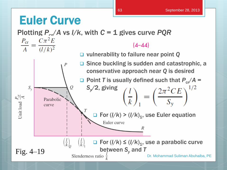
Euler Curve Plotting Pcr/A vs l/k, with C = 1 gives curve PQR
Dr. Mohammad Suliman Abuhaiba, PE Fig. 4–19
September 28, 2013 63
vulnerability to failure near point Q
Since buckling is sudden and catastrophic, a
conservative approach near Q is desired
Point T is usually defined such that Pcr/A =
Sy/2, giving
For (l/k) > (l/k)1, use Euler equation
For (l/k) ≤ (l/k)1, use a parabolic curve
between Sy and T
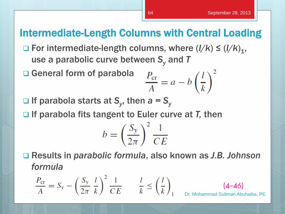
Intermediate-Length Columns with Central Loading
For intermediate-length columns, where (l/k) ≤ (l/k)1,
use a parabolic curve between Sy and T
General form of parabola
If parabola starts at Sy, then a = Sy
If parabola fits tangent to Euler curve at T, then
Results in parabolic formula, also known as J.B. Johnson
formula
Dr. Mohammad Suliman Abuhaiba, PE
September 28, 2013 64
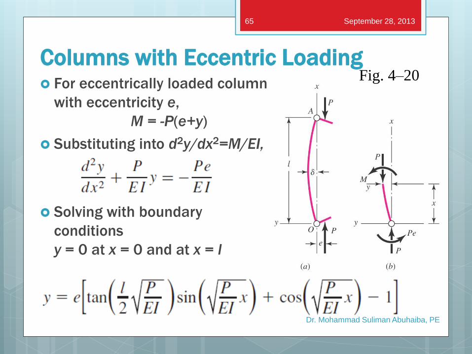
Columns with Eccentric Loading For eccentrically loaded column
with eccentricity e,
M = -P(e+y)
Substituting into d2y/dx2=M/EI,
Solving with boundary
conditions
y = 0 at x = 0 and at x = l
Dr. Mohammad Suliman Abuhaiba, PE
Fig. 4–20
September 28, 2013 65
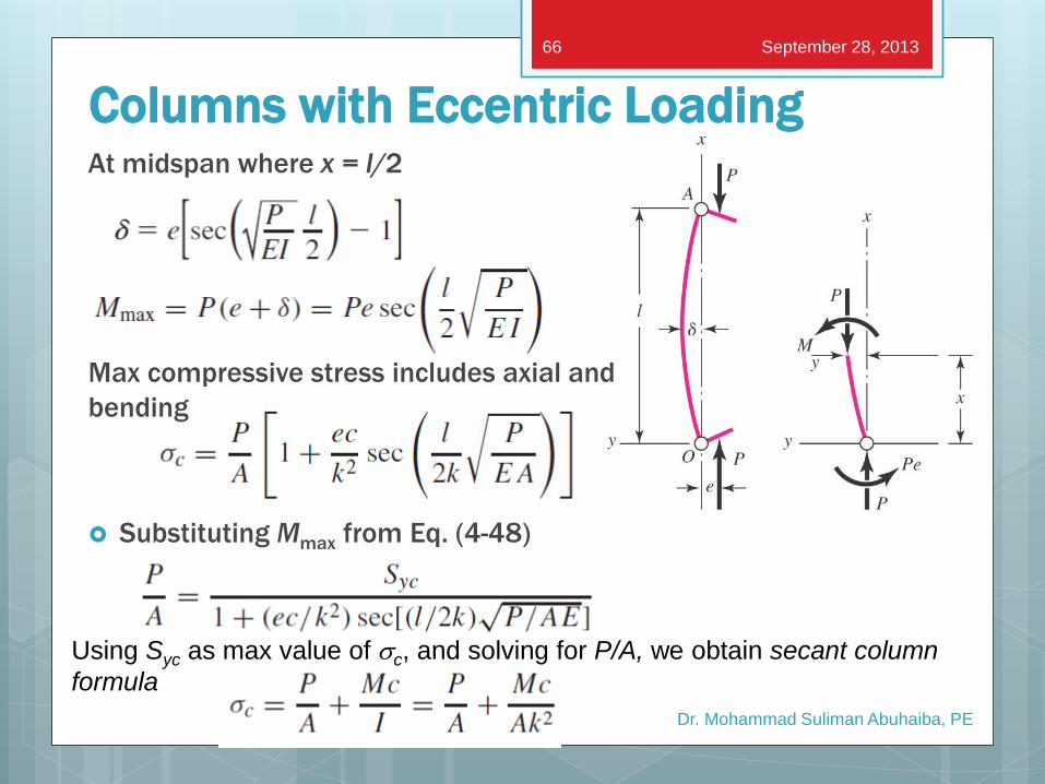
At midspan where x = l/2
Max compressive stress includes axial and
bending
Substituting Mmax from Eq. (4-48)
Dr. Mohammad Suliman Abuhaiba, PE
September 28, 2013 66
Columns with Eccentric Loading
Using Syc as max value of sc, and solving for P/A, we obtain secant column
formula
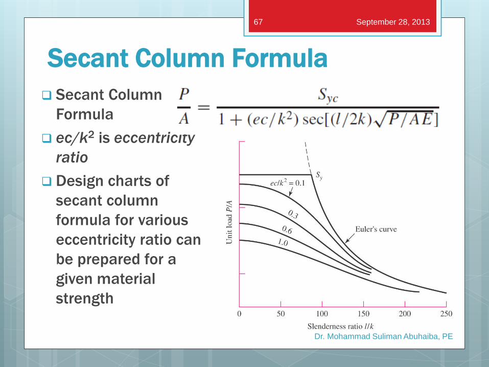
Secant Column Formula
Secant Column
Formula
ec/k2 is eccentricity
ratio
Design charts of
secant column
formula for various
eccentricity ratio can
be prepared for a
given material
strength
Dr. Mohammad Suliman Abuhaiba, PE
Fig. 4–21
September 28, 2013 67
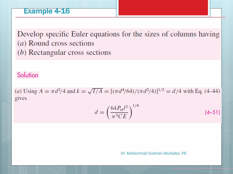
Example 4-16
Dr. Mohammad Suliman Abuhaiba, PE

Example 4-16
Dr. Mohammad Suliman Abuhaiba, PE

Chapter 5
Failures Resulting from
Static Loading
September 28, 2013
Dr. Mohammad Suliman Abuhaiba, PE
70
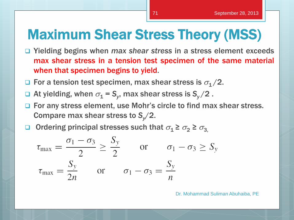
Maximum Shear Stress Theory (MSS) Yielding begins when max shear stress in a stress element exceeds
max shear stress in a tension test specimen of the same material
when that specimen begins to yield.
For a tension test specimen, max shear stress is s1 /2.
At yielding, when s1 = Sy, max shear stress is Sy /2 .
For any stress element, use Mohr’s circle to find max shear stress.
Compare max shear stress to Sy/2.
Ordering principal stresses such that s1 ≥ s2 ≥ s3,
Dr. Mohammad Suliman Abuhaiba, PE
September 28, 2013 71
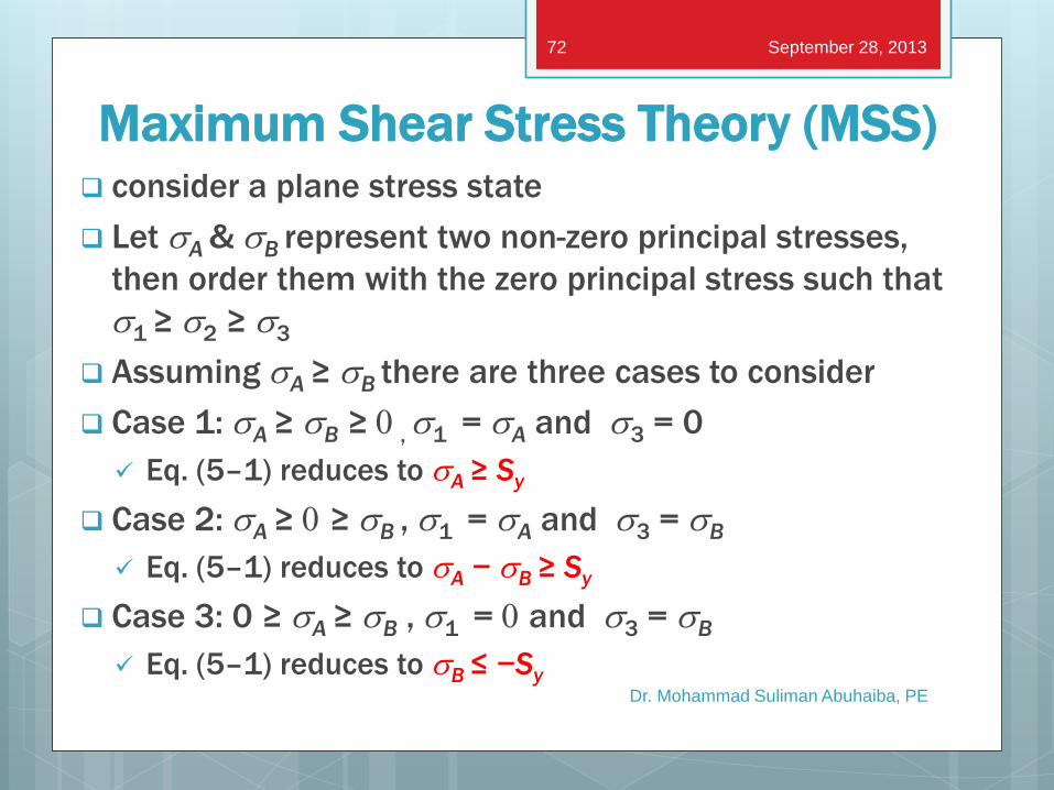
consider a plane stress state
Let sA & sB represent two non-zero principal stresses,
then order them with the zero principal stress such that
s1 ≥ s2 ≥ s3
Assuming sA ≥ sB there are three cases to consider
Case 1: sA ≥ sB ≥ 0 , s1 = sA and s3 = 0
Eq. (5–1) reduces to sA ≥ Sy
Case 2: sA ≥ 0 ≥ sB , s1 = sA and s3 = sB
Eq. (5–1) reduces to sA − sB ≥ Sy
Case 3: 0 ≥ sA ≥ sB , s1 = 0 and s3 = sB
Eq. (5–1) reduces to sB ≤ −Sy
Dr. Mohammad Suliman Abuhaiba, PE
September 28, 2013 72
Maximum Shear Stress Theory (MSS)
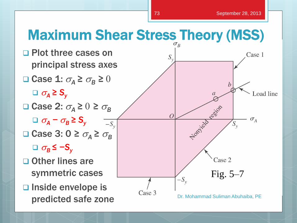
Plot three cases on
principal stress axes
Case 1: sA ≥ sB ≥ 0
sA ≥ Sy
Case 2: sA ≥ 0 ≥ sB
sA − sB ≥ Sy
Case 3: 0 ≥ sA ≥ sB
sB ≤ −Sy
Other lines are
symmetric cases
Inside envelope is
predicted safe zone
Dr. Mohammad Suliman Abuhaiba, PE
Fig. 5–7
September 28, 2013 73
Maximum Shear Stress Theory (MSS)
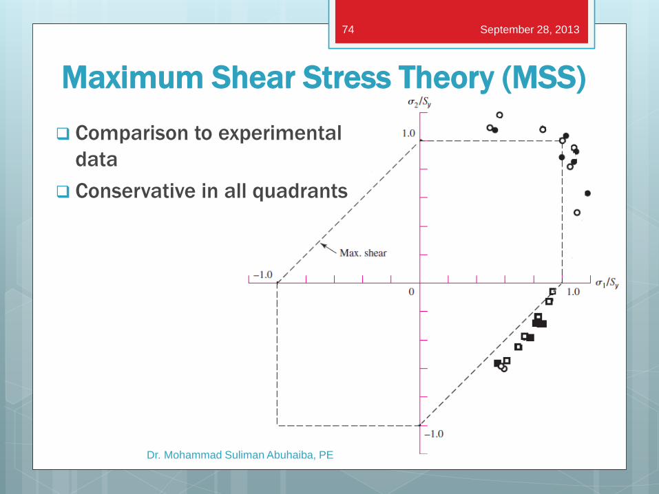
Comparison to experimental
data
Conservative in all quadrants
Dr. Mohammad Suliman Abuhaiba, PE
September 28, 2013 74
Maximum Shear Stress Theory (MSS)
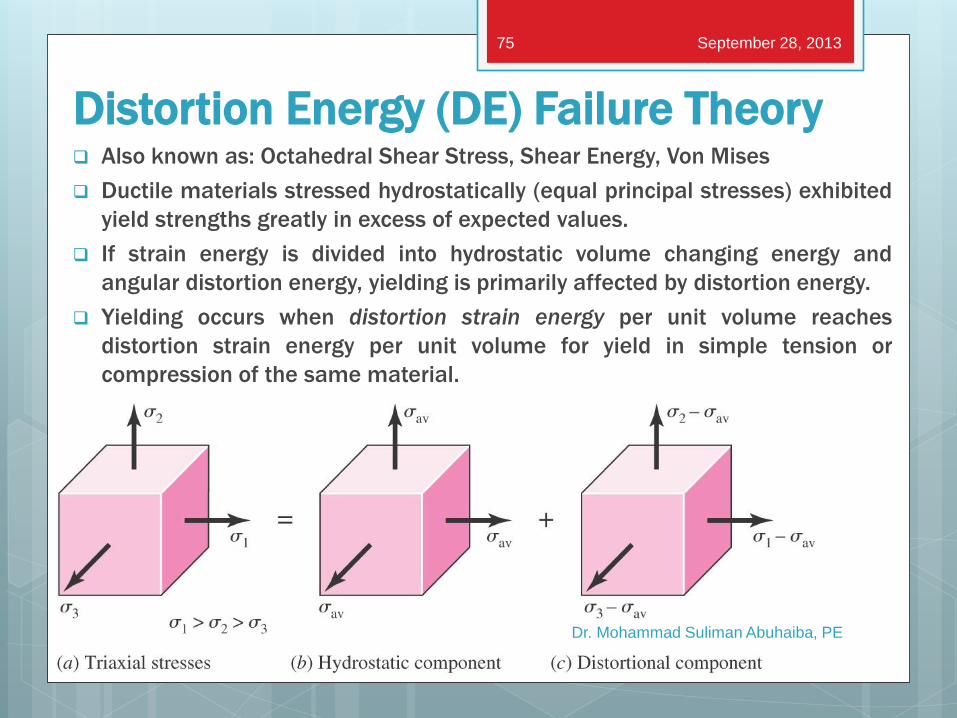
Distortion Energy (DE) Failure Theory Also known as: Octahedral Shear Stress, Shear Energy, Von Mises
Ductile materials stressed hydrostatically (equal principal stresses) exhibited
yield strengths greatly in excess of expected values.
If strain energy is divided into hydrostatic volume changing energy and
angular distortion energy, yielding is primarily affected by distortion energy.
Yielding occurs when distortion strain energy per unit volume reaches
distortion strain energy per unit volume for yield in simple tension or
compression of the same material.
Dr. Mohammad Suliman Abuhaiba, PE
September 28, 2013 75
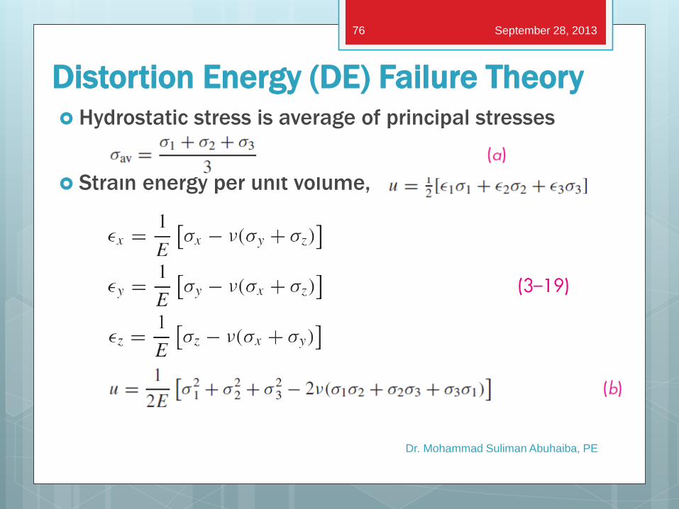
Hydrostatic stress is average of principal stresses
Strain energy per unit volume,
Dr. Mohammad Suliman Abuhaiba, PE
September 28, 2013 76
Distortion Energy (DE) Failure Theory
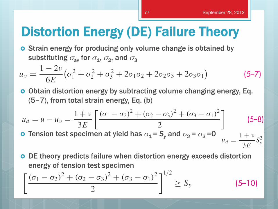
Strain energy for producing only volume change is obtained by
substituting sav for s1, s2, and s3
Obtain distortion energy by subtracting volume changing energy, Eq.
(5–7), from total strain energy, Eq. (b)
Tension test specimen at yield has s1 = Sy and s2 = s3 =0
DE theory predicts failure when distortion energy exceeds distortion
energy of tension test specimen
Dr. Mohammad Suliman Abuhaiba, PE
September 28, 2013 77
Distortion Energy (DE) Failure Theory
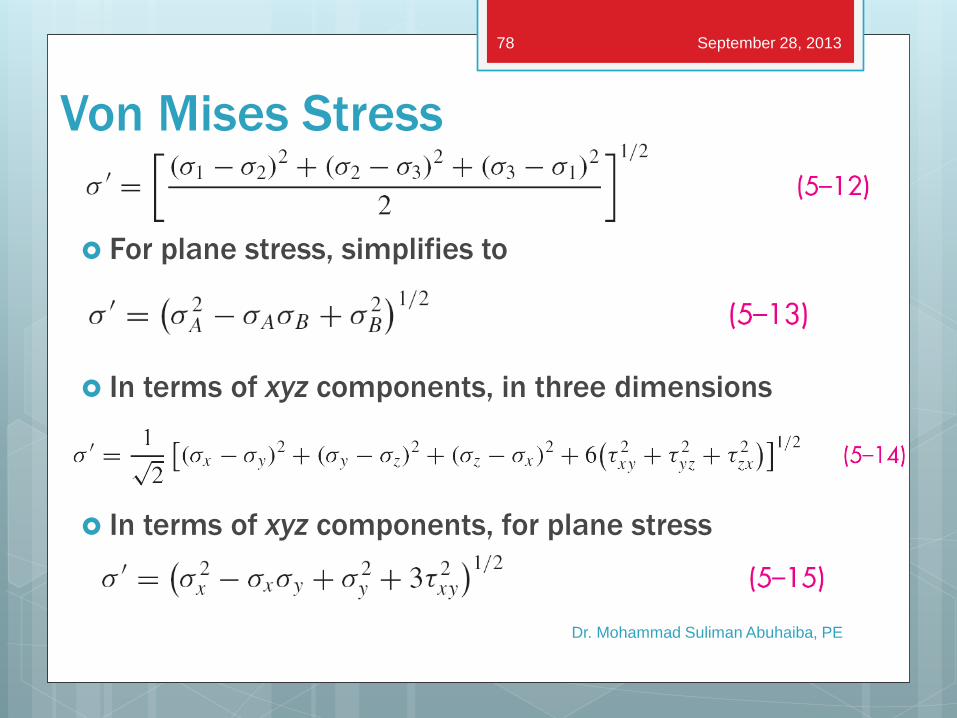
Von Mises Stress
For plane stress, simplifies to
In terms of xyz components, in three dimensions
In terms of xyz components, for plane stress
Dr. Mohammad Suliman Abuhaiba, PE
September 28, 2013 78
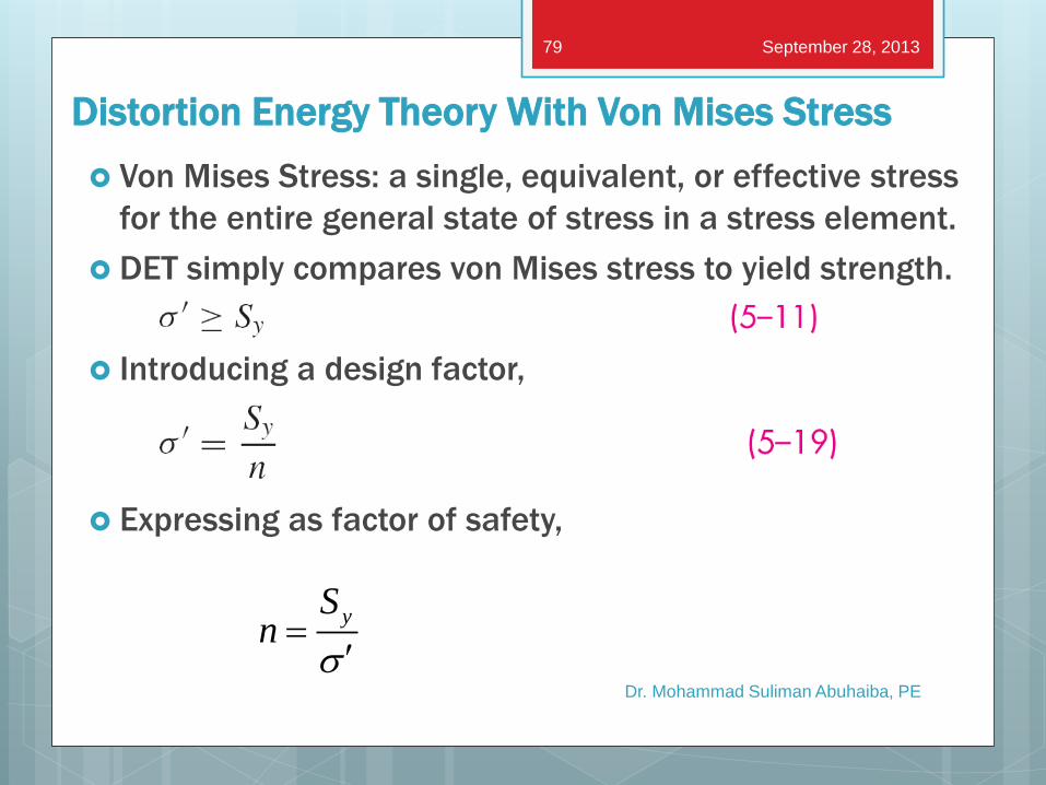
Distortion Energy Theory With Von Mises Stress
Von Mises Stress: a single, equivalent, or effective stress
for the entire general state of stress in a stress element.
DET simply compares von Mises stress to yield strength.
Introducing a design factor,
Expressing as factor of safety,
Dr. Mohammad Suliman Abuhaiba, PE
ySn
s
September 28, 2013 79
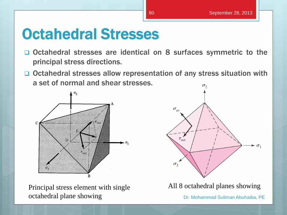
Octahedral Stresses Octahedral stresses are identical on 8 surfaces symmetric to the
principal stress directions.
Octahedral stresses allow representation of any stress situation with
a set of normal and shear stresses.
Dr. Mohammad Suliman Abuhaiba, PE
Principal stress element with single
octahedral plane showing
All 8 octahedral planes showing
September 28, 2013 80
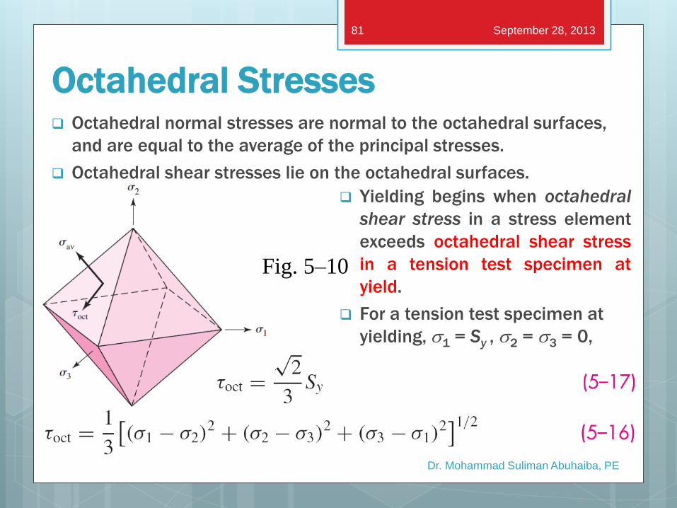
Octahedral normal stresses are normal to the octahedral surfaces,
and are equal to the average of the principal stresses.
Octahedral shear stresses lie on the octahedral surfaces.
Dr. Mohammad Suliman Abuhaiba, PE
Fig. 5–10
September 28, 2013 81
Octahedral Stresses
Yielding begins when octahedral
shear stress in a stress element
exceeds octahedral shear stress
in a tension test specimen at
yield.
For a tension test specimen at
yielding, s1 = Sy , s2 = s3 = 0,
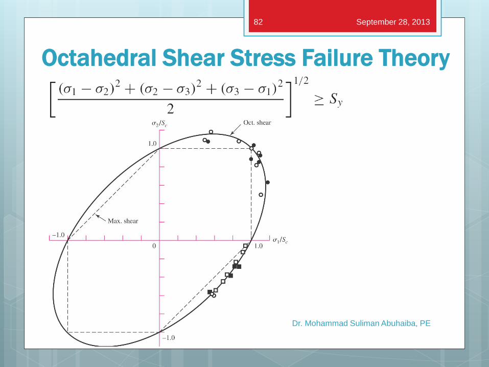
Octahedral Shear Stress Failure Theory
Dr. Mohammad Suliman Abuhaiba, PE
September 28, 2013 82
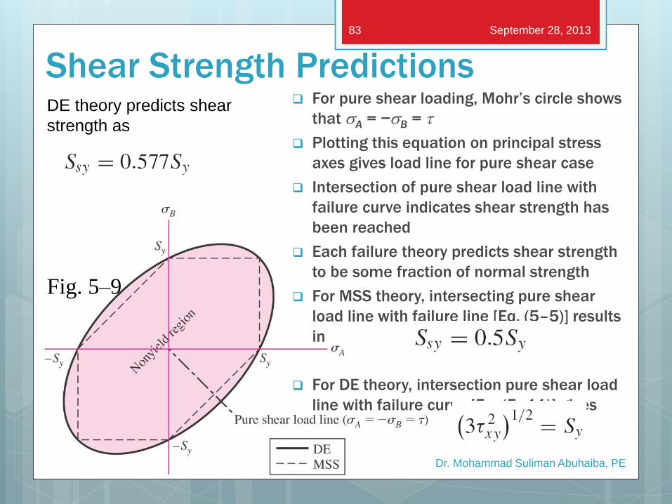
Shear Strength Predictions For pure shear loading, Mohr’s circle shows
that sA = −sB = t
Plotting this equation on principal stress
axes gives load line for pure shear case
Intersection of pure shear load line with
failure curve indicates shear strength has
been reached
Each failure theory predicts shear strength
to be some fraction of normal strength
For MSS theory, intersecting pure shear
load line with failure line [Eq. (5–5)] results
in
For DE theory, intersection pure shear load
line with failure curve [Eq. (5–11)] gives
Dr. Mohammad Suliman Abuhaiba, PE
Fig. 5–9
September 28, 2013 83
DE theory predicts shear
strength as
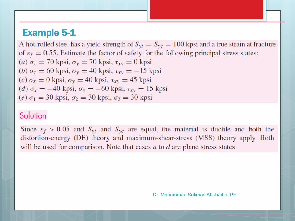
Example 5-1
Dr. Mohammad Suliman Abuhaiba, PE
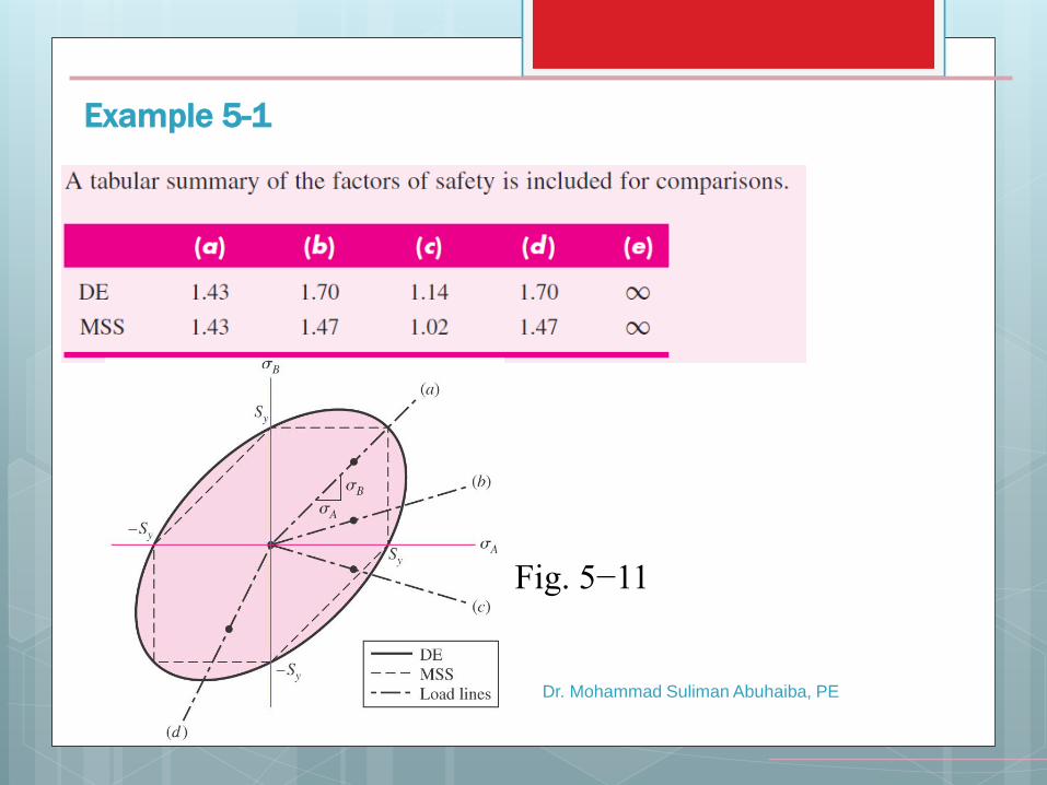
Example 5-1
Dr. Mohammad Suliman Abuhaiba, PE
Fig. 5−11
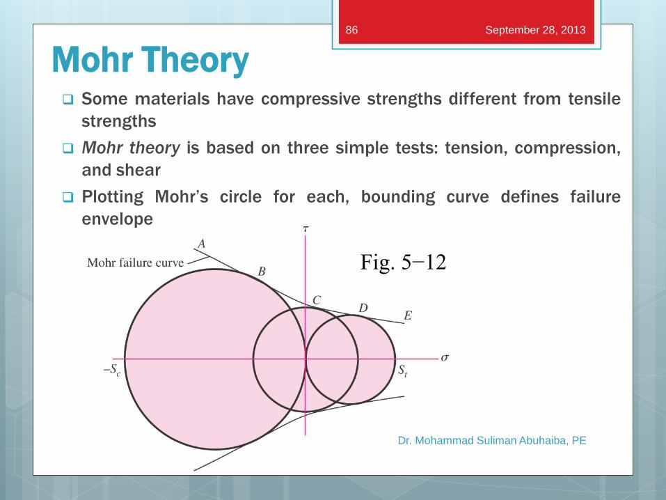
Mohr Theory Some materials have compressive strengths different from tensile
strengths
Mohr theory is based on three simple tests: tension, compression,
and shear
Plotting Mohr’s circle for each, bounding curve defines failure
envelope
Dr. Mohammad Suliman Abuhaiba, PE
Fig. 5−12
September 28, 2013 86

Coulomb-Mohr Theory Curved failure curve is difficult
to determine analytically
Coulomb-Mohr theory
simplifies to linear failure
envelope using only tension
and compression tests
(dashed circles)
Dr. Mohammad Suliman Abuhaiba, PE
Fig. 5−13
September 28, 2013 87
For ductile material, use tensile
and compressive yield strengths
For brittle material, use tensile
&compressive ultimate strengths
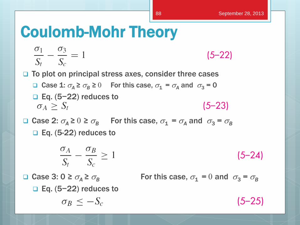
To plot on principal stress axes, consider three cases
Case 1: sA ≥ sB ≥ 0 For this case, s1 = sA and s3 = 0
Eq. (5−22) reduces to
Case 2: sA ≥ 0 ≥ sB For this case, s1 = sA and s3 = sB
Eq. (5-22) reduces to
Case 3: 0 ≥ sA ≥ sB For this case, s1 = 0 and s3 = sB
Eq. (5−22) reduces to
Dr. Mohammad Suliman Abuhaiba, PE
September 28, 2013 88
Coulomb-Mohr Theory
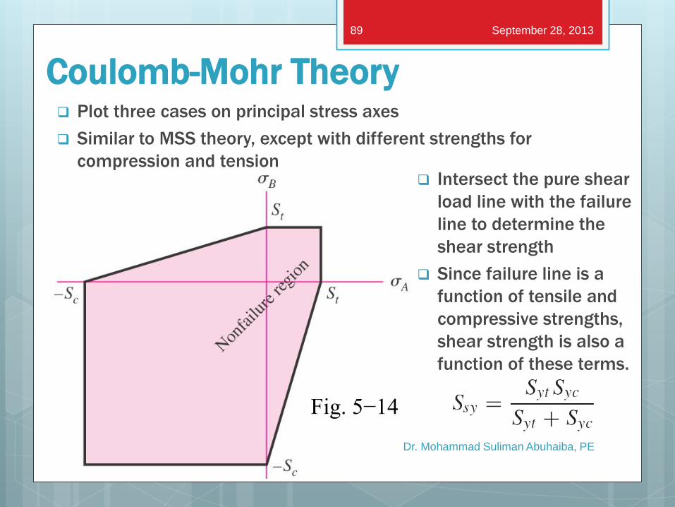
Plot three cases on principal stress axes
Similar to MSS theory, except with different strengths for
compression and tension
Dr. Mohammad Suliman Abuhaiba, PE
Fig. 5−14
September 28, 2013 89
Coulomb-Mohr Theory
Intersect the pure shear
load line with the failure
line to determine the
shear strength
Since failure line is a
function of tensile and
compressive strengths,
shear strength is also a
function of these terms.
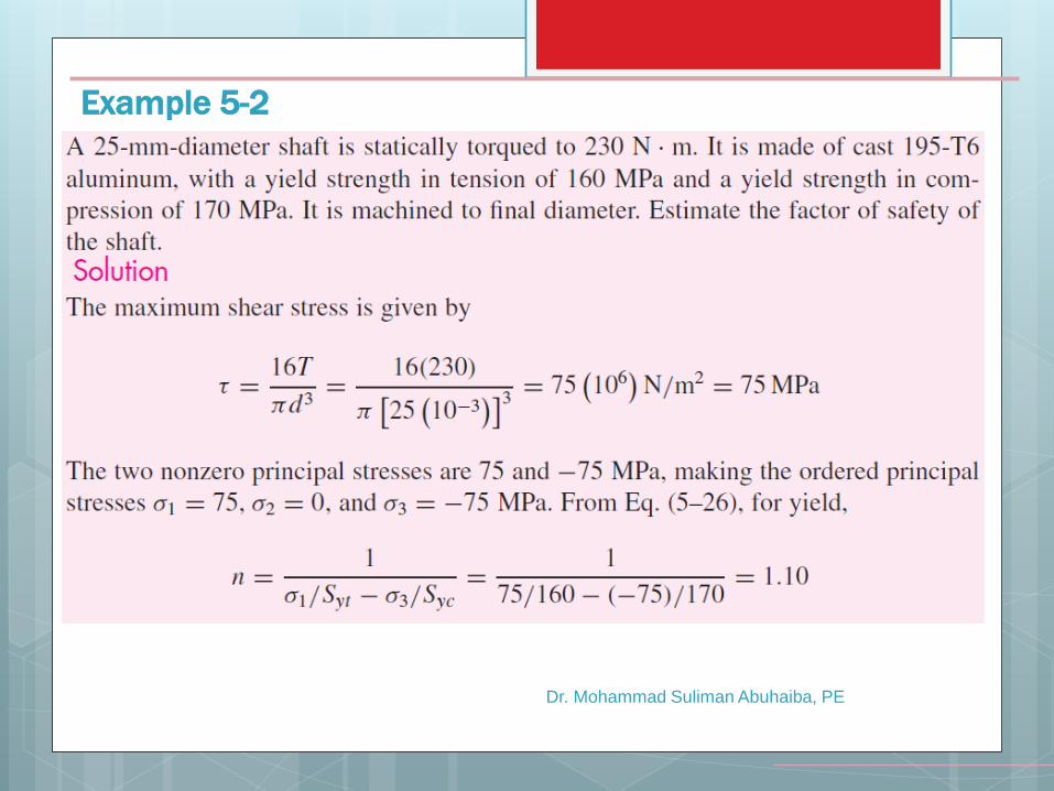
Example 5-2
Dr. Mohammad Suliman Abuhaiba, PE
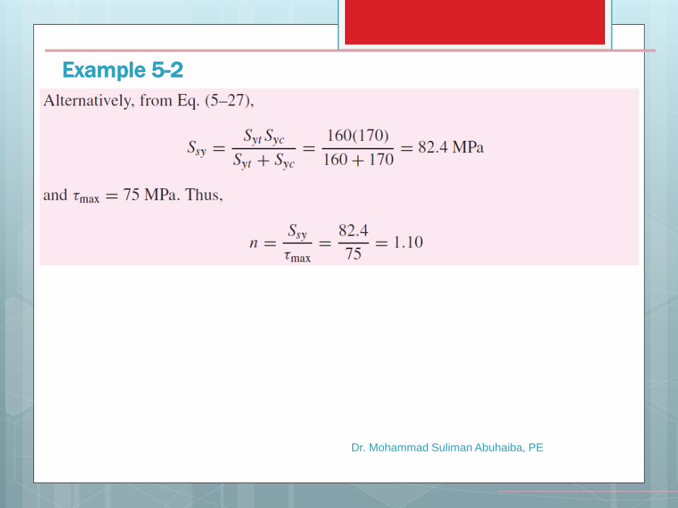
Example 5-2
Dr. Mohammad Suliman Abuhaiba, PE
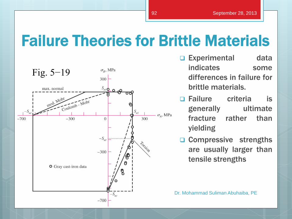
Failure Theories for Brittle Materials Experimental data
indicates some
differences in failure for
brittle materials.
Failure criteria is
generally ultimate
fracture rather than
yielding
Compressive strengths
are usually larger than
tensile strengths
Dr. Mohammad Suliman Abuhaiba, PE
Fig. 5−19
September 28, 2013 92
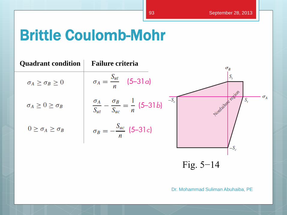
Brittle Coulomb-Mohr
Dr. Mohammad Suliman Abuhaiba, PE
Quadrant condition Failure criteria
Fig. 5−14
September 28, 2013 93
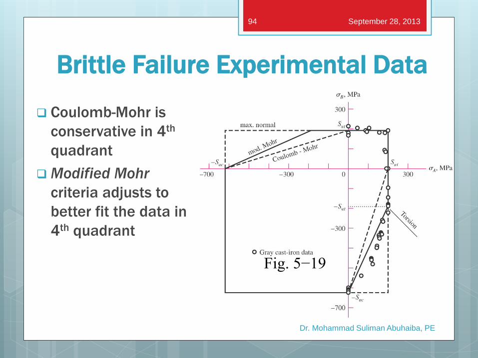
Brittle Failure Experimental Data
Coulomb-Mohr is
conservative in 4th
quadrant
Modified Mohr
criteria adjusts to
better fit the data in
4th quadrant
Dr. Mohammad Suliman Abuhaiba, PE
Fig. 5−19
September 28, 2013 94
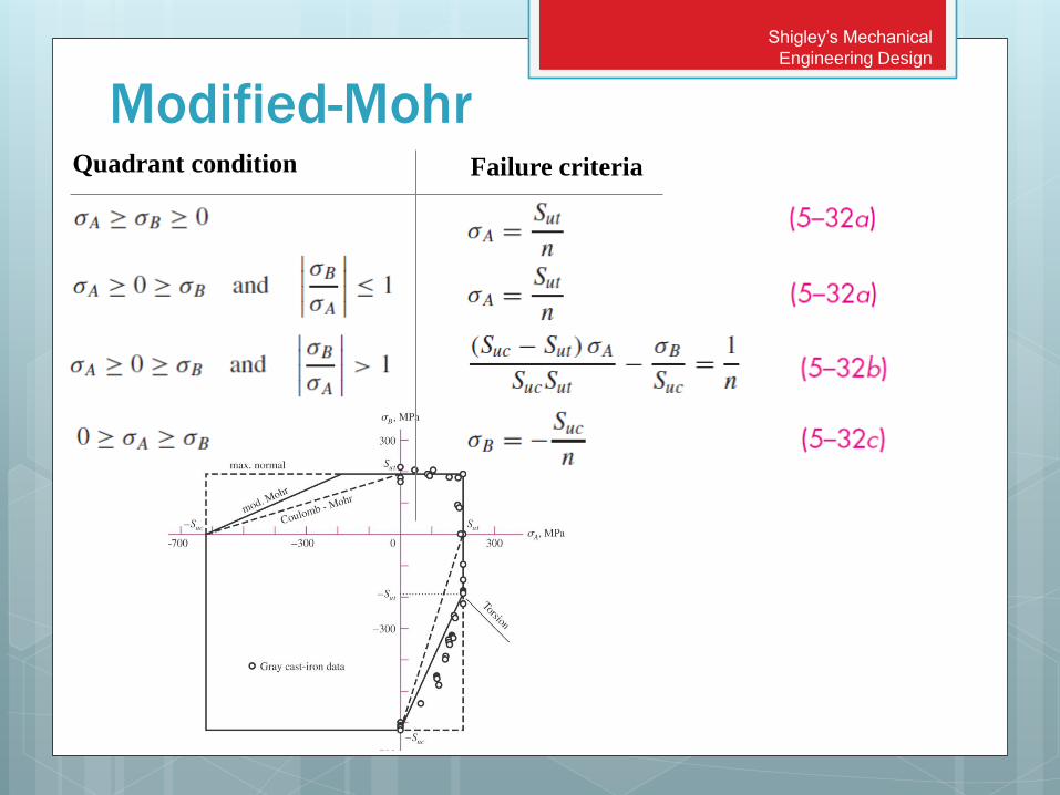
Modified-Mohr
Shigley’s Mechanical
Engineering Design
Quadrant condition Failure criteria
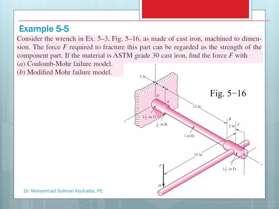
Example 5-5
Dr. Mohammad Suliman Abuhaiba, PE
Fig. 5−16
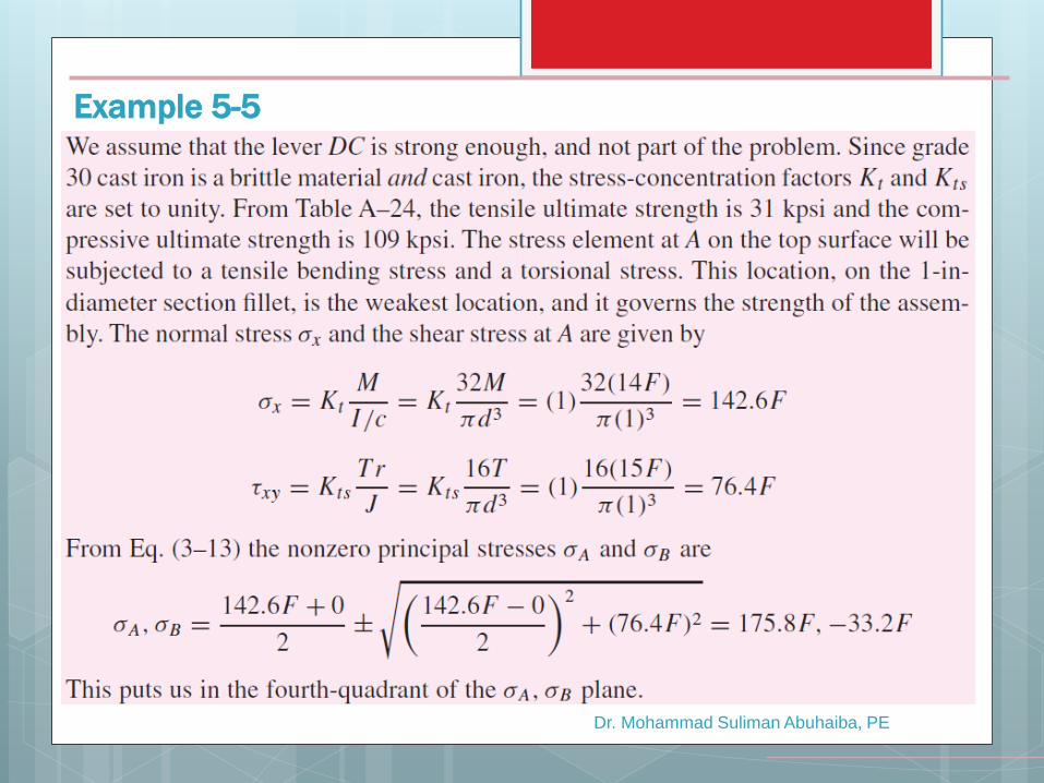
Example 5-5
Dr. Mohammad Suliman Abuhaiba, PE

Example 5-5
Dr. Mohammad Suliman Abuhaiba, PE
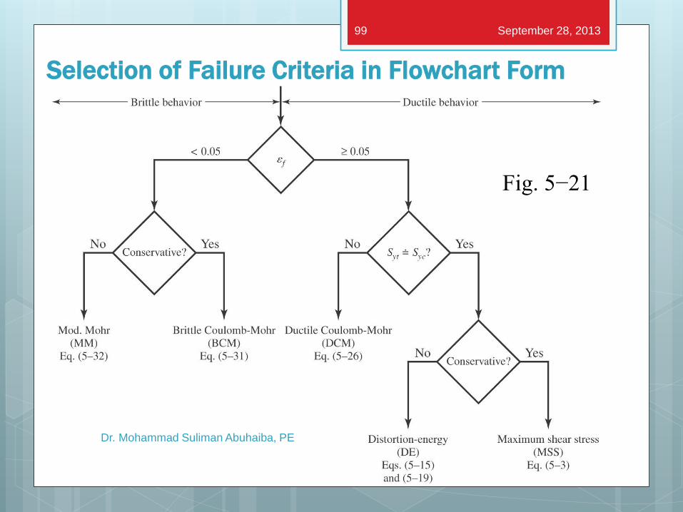
Selection of Failure Criteria in Flowchart Form
Dr. Mohammad Suliman Abuhaiba, PE
Fig. 5−21
September 28, 2013 99
Chapter 6
Fatigue Failure Resulting
from Variable Loading
The McGraw-Hill Companies © 2012
September 28, 2013
Dr. Mohammad Suliman Abuhaiba, PE
100
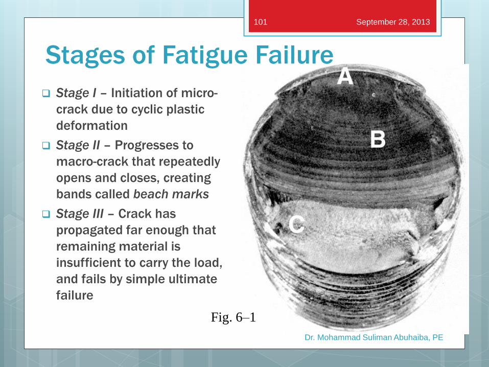
Stages of Fatigue Failure
Stage I – Initiation of micro-
crack due to cyclic plastic
deformation
Stage II – Progresses to
macro-crack that repeatedly
opens and closes, creating
bands called beach marks
Stage III – Crack has
propagated far enough that
remaining material is
insufficient to carry the load,
and fails by simple ultimate
failure
Dr. Mohammad Suliman Abuhaiba, PE
Fig. 6–1
September 28, 2013 101
Fatigue-Life Methods
Three major fatigue life models
Methods predict life in number of cycles to failure, N, for a specific
level of loading
1. Stress-life method
Least accurate, particularly for low cycle applications
Most traditional, easiest to implement
2. Strain-life method
Detailed analysis of plastic deformation at localized regions
Several idealizations are compounded, leading to uncertainties in
results
3. Linear-elastic fracture mechanics method
Assumes crack exists
Predicts crack growth with respect to stress intensity
Dr. Mohammad Suliman Abuhaiba, PE
September 28, 2013 102
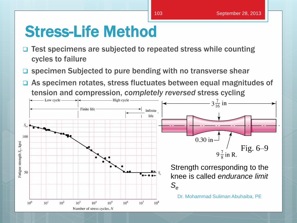
Stress-Life Method Test specimens are subjected to repeated stress while counting
cycles to failure
specimen Subjected to pure bending with no transverse shear
As specimen rotates, stress fluctuates between equal magnitudes of
tension and compression, completely reversed stress cycling
Dr. Mohammad Suliman Abuhaiba, PE
Fig. 6–9
September 28, 2013 103
Strength corresponding to the
knee is called endurance limit
Se
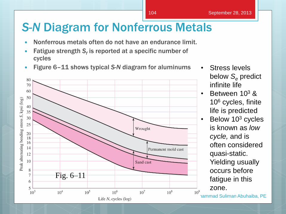
S-N Diagram for Nonferrous Metals Nonferrous metals often do not have an endurance limit.
Fatigue strength Sf is reported at a specific number of cycles
Figure 6–11 shows typical S-N diagram for aluminums
Dr. Mohammad Suliman Abuhaiba, PE
Fig. 6–11
September 28, 2013 104
• Stress levels
below Se predict
infinite life
• Between 103 &
106 cycles, finite
life is predicted
• Below 103 cycles
is known as low
cycle, and is
often considered
quasi-static.
Yielding usually
occurs before
fatigue in this
zone.
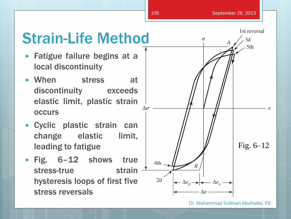
Strain-Life Method Fatigue failure begins at a
local discontinuity
When stress at
discontinuity exceeds
elastic limit, plastic strain
occurs
Cyclic plastic strain can
change elastic limit,
leading to fatigue
Fig. 6–12 shows true
stress-true strain
hysteresis loops of first five
stress reversals
Dr. Mohammad Suliman Abuhaiba, PE
Fig. 6–12
September 28, 2013 105
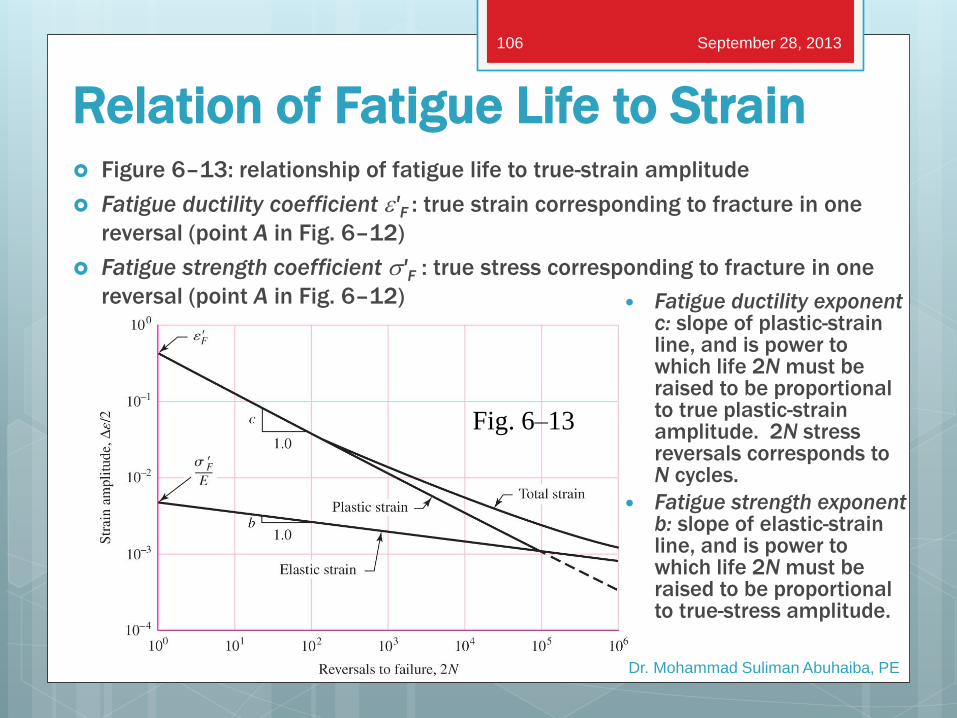
Relation of Fatigue Life to Strain Figure 6–13: relationship of fatigue life to true-strain amplitude
Fatigue ductility coefficient e'F : true strain corresponding to fracture in one
reversal (point A in Fig. 6–12)
Fatigue strength coefficient s'F : true stress corresponding to fracture in one
reversal (point A in Fig. 6–12)
Dr. Mohammad Suliman Abuhaiba, PE
Fig. 6–13
September 28, 2013 106
Fatigue ductility exponent c: slope of plastic-strain line, and is power to which life 2N must be raised to be proportional to true plastic-strain amplitude. 2N stress reversals corresponds to N cycles.
Fatigue strength exponent b: slope of elastic-strain line, and is power to which life 2N must be raised to be proportional to true-stress amplitude.
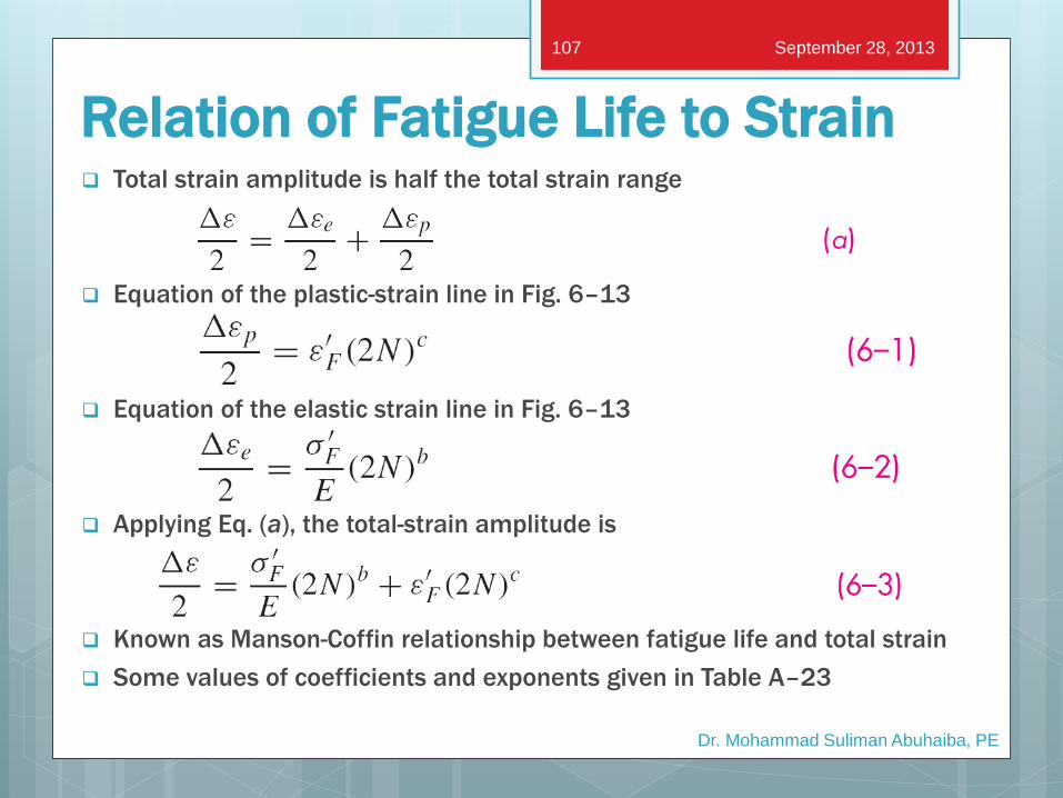
Total strain amplitude is half the total strain range
Equation of the plastic-strain line in Fig. 6–13
Equation of the elastic strain line in Fig. 6–13
Applying Eq. (a), the total-strain amplitude is
Known as Manson-Coffin relationship between fatigue life and total strain
Some values of coefficients and exponents given in Table A–23
Dr. Mohammad Suliman Abuhaiba, PE
September 28, 2013 107
Relation of Fatigue Life to Strain
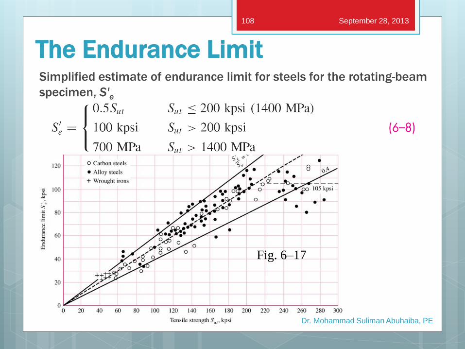
The Endurance Limit Simplified estimate of endurance limit for steels for the rotating-beam
specimen, S'e
Dr. Mohammad Suliman Abuhaiba, PE
Fig. 6–17
September 28, 2013 108
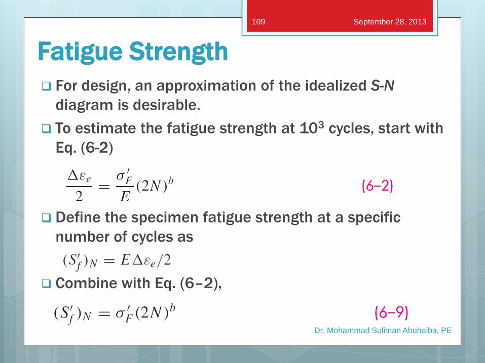
Fatigue Strength
For design, an approximation of the idealized S-N
diagram is desirable.
To estimate the fatigue strength at 103 cycles, start with
Eq. (6-2)
Define the specimen fatigue strength at a specific
number of cycles as
Combine with Eq. (6–2),
Dr. Mohammad Suliman Abuhaiba, PE
September 28, 2013 109
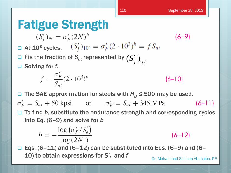
At 103 cycles,
f is the fraction of Sut represented by
Solving for f,
The SAE approximation for steels with HB ≤ 500 may be used.
To find b, substitute the endurance strength and corresponding cycles
into Eq. (6–9) and solve for b
Eqs. (6–11) and (6–12) can be substituted into Eqs. (6–9) and (6–
10) to obtain expressions for S'f and f
Dr. Mohammad Suliman Abuhaiba, PE
310( )fS
September 28, 2013 110
Fatigue Strength
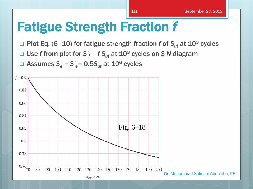
Fatigue Strength Fraction f Plot Eq. (6–10) for fatigue strength fraction f of Sut at 103 cycles
Use f from plot for S'f = f Sut at 103 cycles on S-N diagram
Assumes Se = S'e= 0.5Sut at 106 cycles
Dr. Mohammad Suliman Abuhaiba, PE
Fig. 6–18
September 28, 2013 111
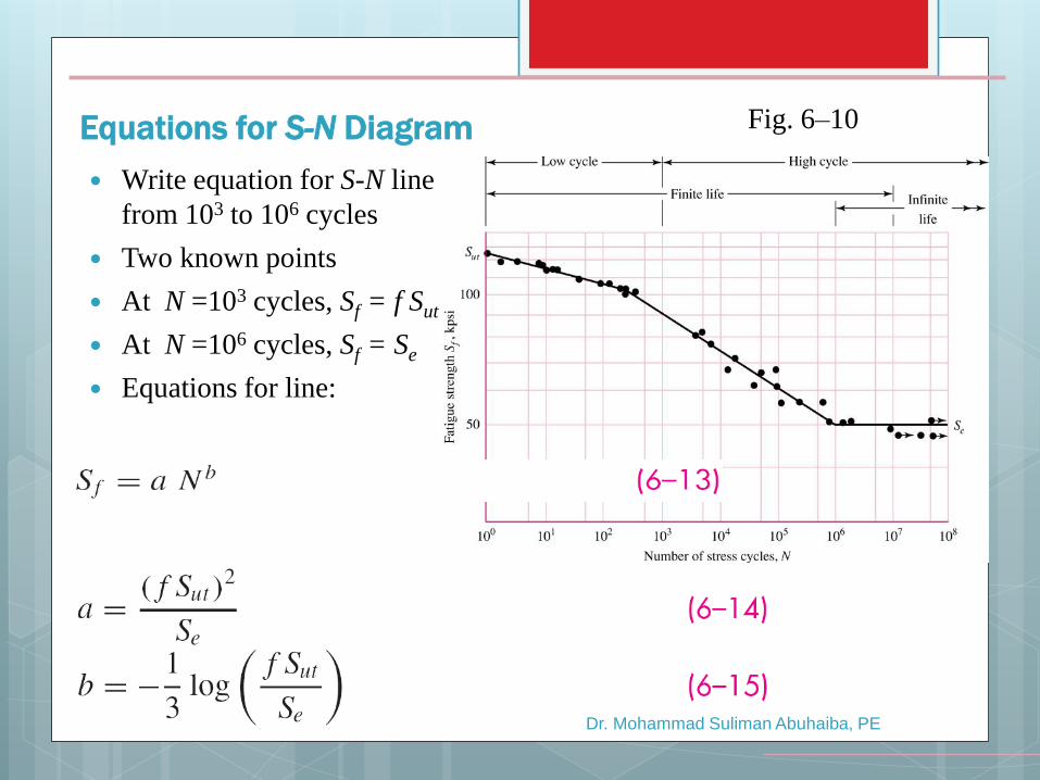
Equations for S-N Diagram
Dr. Mohammad Suliman Abuhaiba, PE
Write equation for S-N line
from 103 to 106 cycles
Two known points
At N =103 cycles, Sf = f Sut
At N =106 cycles, Sf = Se
Equations for line:
Fig. 6–10
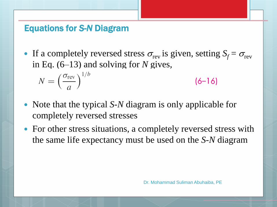
Equations for S-N Diagram
Dr. Mohammad Suliman Abuhaiba, PE
If a completely reversed stress srev is given, setting Sf = srev
in Eq. (6–13) and solving for N gives,
Note that the typical S-N diagram is only applicable for
completely reversed stresses
For other stress situations, a completely reversed stress with
the same life expectancy must be used on the S-N diagram
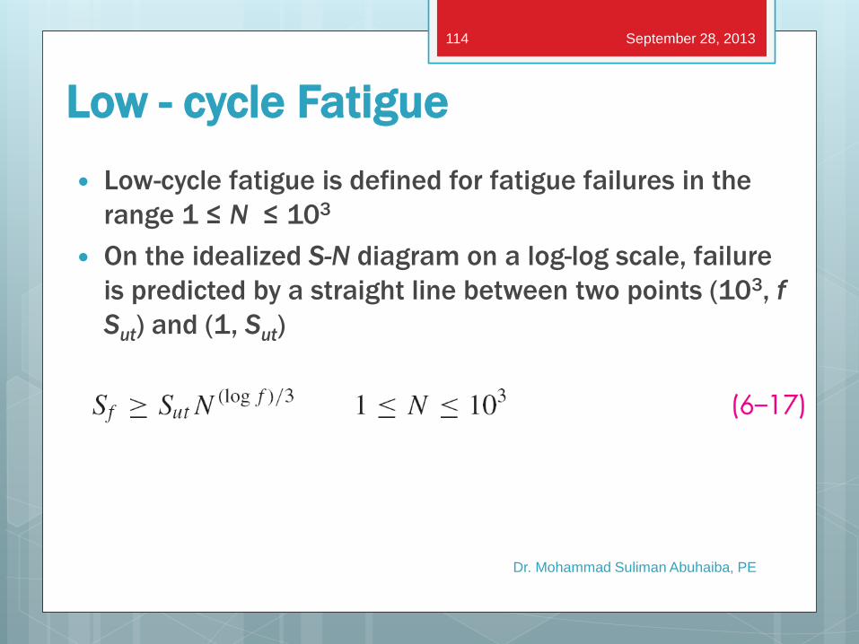
Low - cycle Fatigue
Low-cycle fatigue is defined for fatigue failures in the
range 1 ≤ N ≤ 103
On the idealized S-N diagram on a log-log scale, failure
is predicted by a straight line between two points (103, f
Sut) and (1, Sut)
Dr. Mohammad Suliman Abuhaiba, PE
September 28, 2013 114
Dr. Mohammad Suliman Abuhaiba, PE
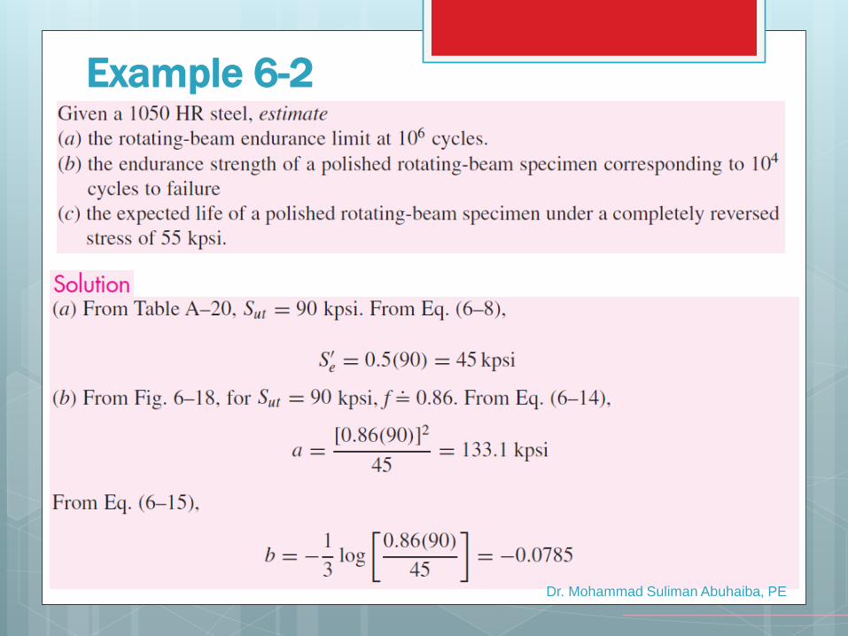
Example 6-2
Dr. Mohammad Suliman Abuhaiba, PE
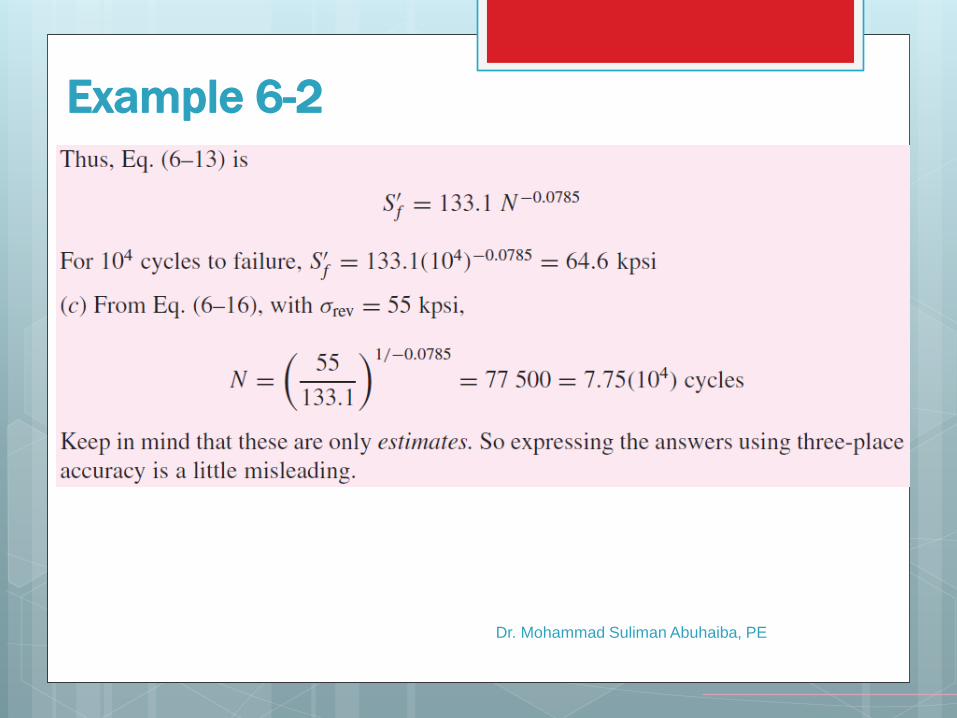
Example 6-2
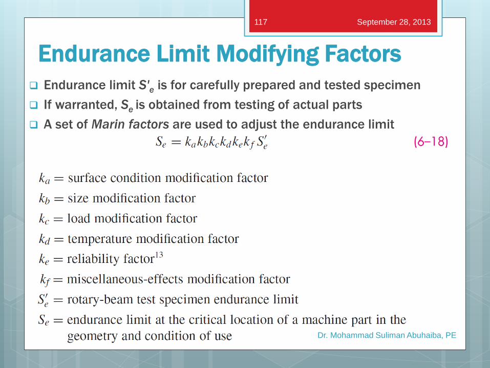
Endurance Limit Modifying Factors
Endurance limit S'e is for carefully prepared and tested specimen
If warranted, Se is obtained from testing of actual parts
A set of Marin factors are used to adjust the endurance limit
Dr. Mohammad Suliman Abuhaiba, PE
September 28, 2013 117
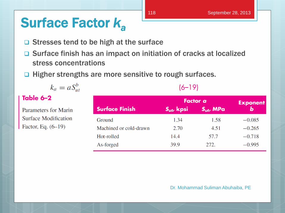
Surface Factor ka
Stresses tend to be high at the surface
Surface finish has an impact on initiation of cracks at localized
stress concentrations
Higher strengths are more sensitive to rough surfaces.
Dr. Mohammad Suliman Abuhaiba, PE
September 28, 2013 118
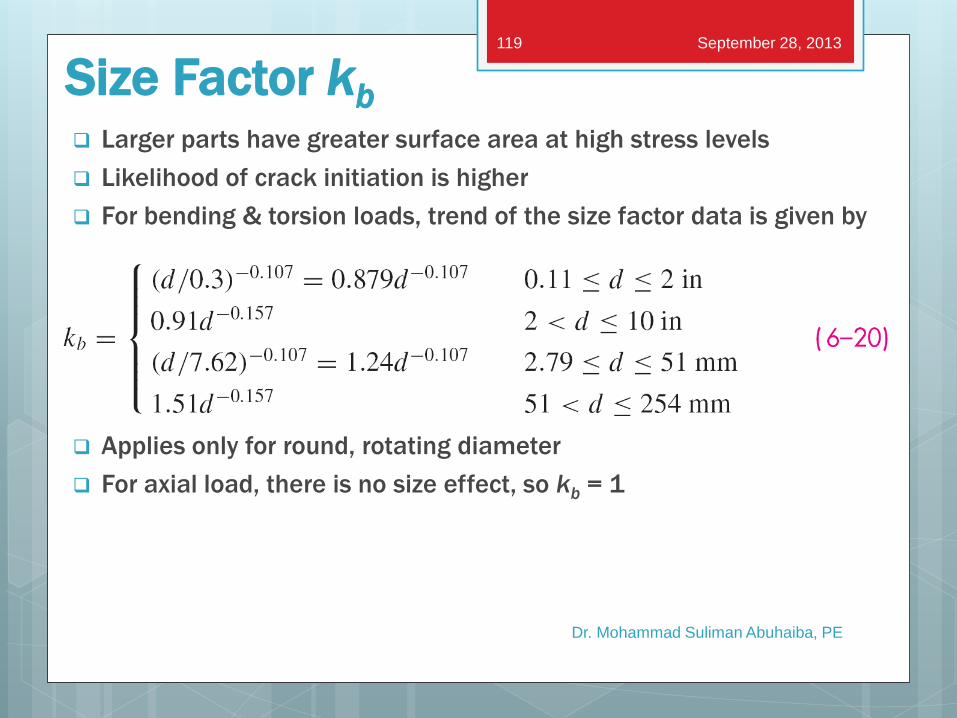
Size Factor kb Larger parts have greater surface area at high stress levels
Likelihood of crack initiation is higher
For bending & torsion loads, trend of the size factor data is given by
Applies only for round, rotating diameter
For axial load, there is no size effect, so kb = 1
Dr. Mohammad Suliman Abuhaiba, PE
September 28, 2013 119
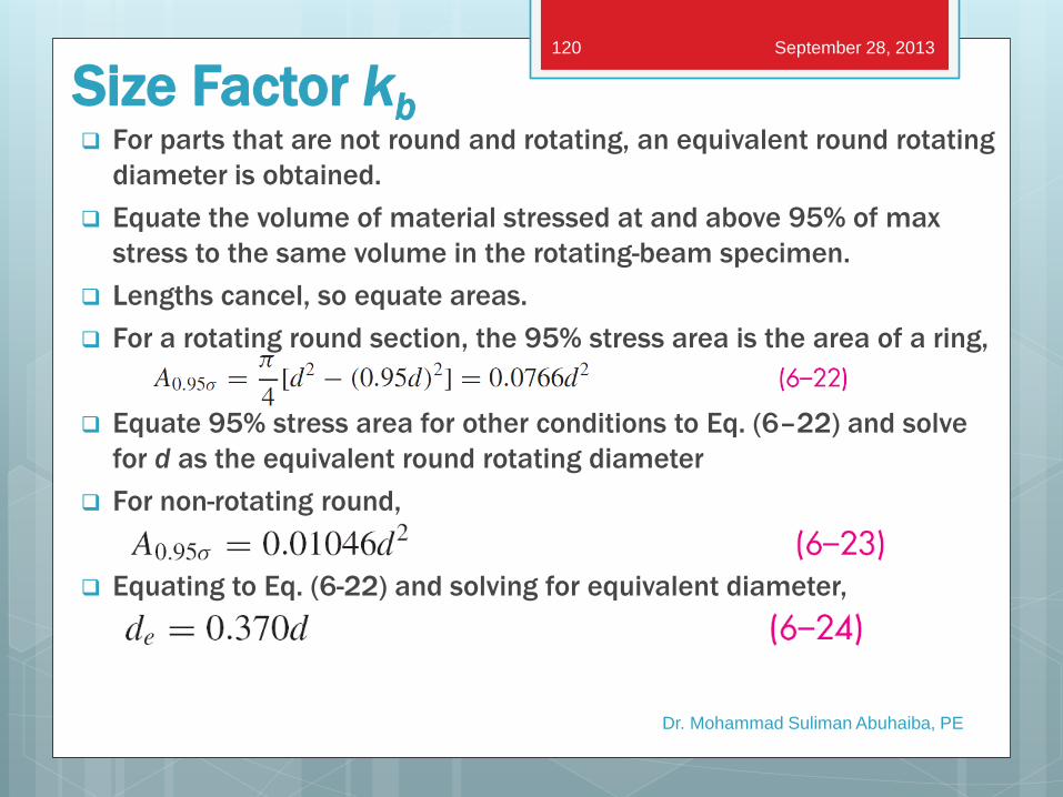
Size Factor kb For parts that are not round and rotating, an equivalent round rotating
diameter is obtained.
Equate the volume of material stressed at and above 95% of max
stress to the same volume in the rotating-beam specimen.
Lengths cancel, so equate areas.
For a rotating round section, the 95% stress area is the area of a ring,
Equate 95% stress area for other conditions to Eq. (6–22) and solve
for d as the equivalent round rotating diameter
For non-rotating round,
Equating to Eq. (6-22) and solving for equivalent diameter,
Dr. Mohammad Suliman Abuhaiba, PE
September 28, 2013 120
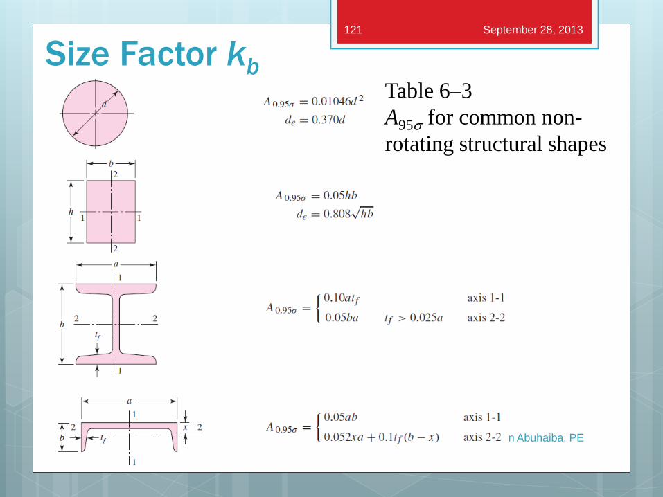
Size Factor kb
Dr. Mohammad Suliman Abuhaiba, PE
Table 6–3
A95s for common non-
rotating structural shapes
September 28, 2013 121
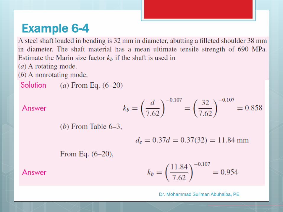
Dr. Mohammad Suliman Abuhaiba, PE
Example 6-4
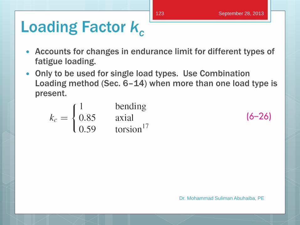
Loading Factor kc
Accounts for changes in endurance limit for different types of fatigue loading.
Only to be used for single load types. Use Combination Loading method (Sec. 6–14) when more than one load type is present.
Dr. Mohammad Suliman Abuhaiba, PE
September 28, 2013 123
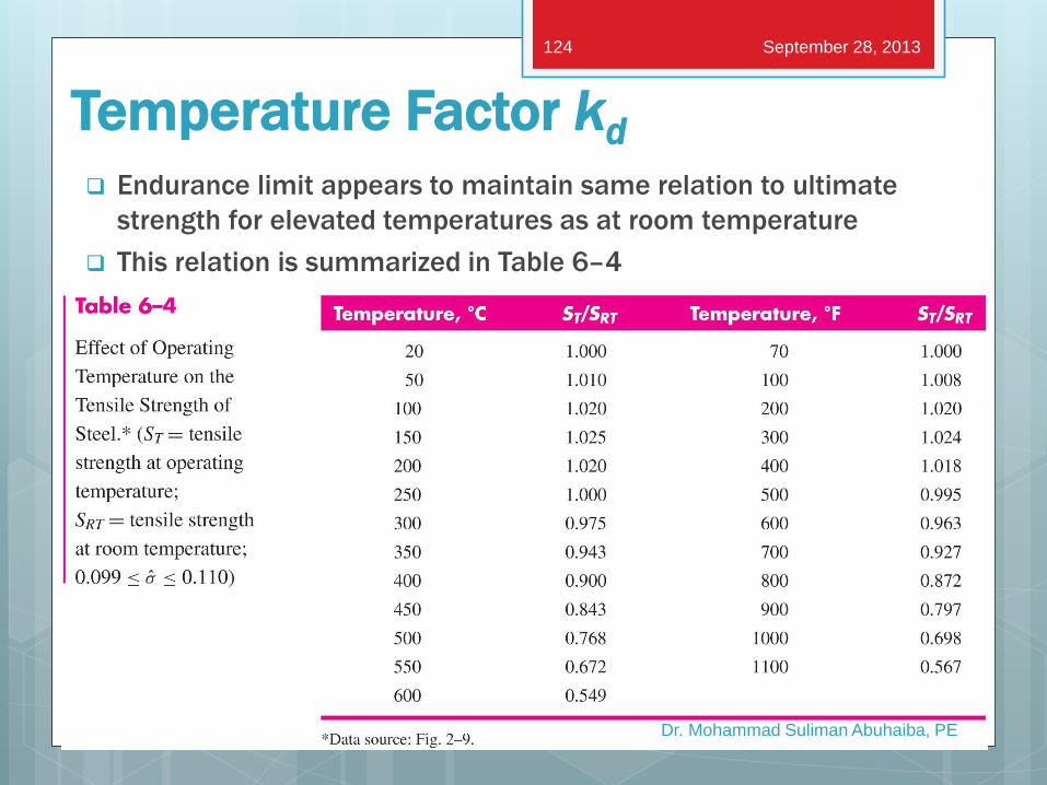
Temperature Factor kd
Endurance limit appears to maintain same relation to ultimate
strength for elevated temperatures as at room temperature
This relation is summarized in Table 6–4
Dr. Mohammad Suliman Abuhaiba, PE
September 28, 2013 124
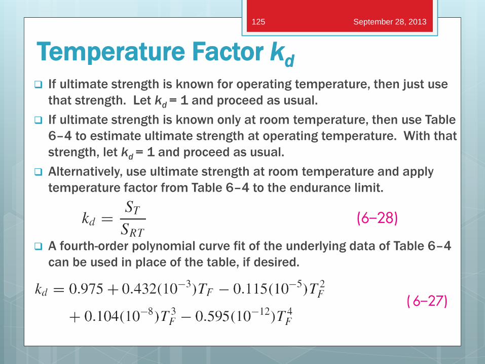
Temperature Factor kd If ultimate strength is known for operating temperature, then just use
that strength. Let kd = 1 and proceed as usual.
If ultimate strength is known only at room temperature, then use Table
6–4 to estimate ultimate strength at operating temperature. With that
strength, let kd = 1 and proceed as usual.
Alternatively, use ultimate strength at room temperature and apply
temperature factor from Table 6–4 to the endurance limit.
A fourth-order polynomial curve fit of the underlying data of Table 6–4
can be used in place of the table, if desired.
Dr. Mohammad Suliman Abuhaiba, PE
September 28, 2013 125
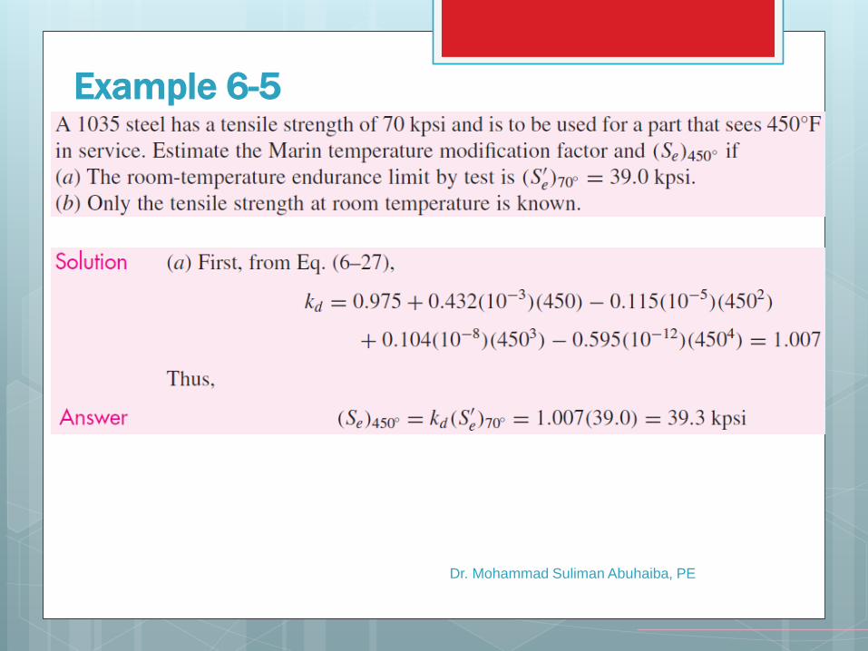
Dr. Mohammad Suliman Abuhaiba, PE
Example 6-5
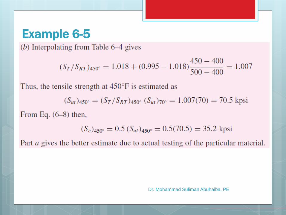
Dr. Mohammad Suliman Abuhaiba, PE
Example 6-5
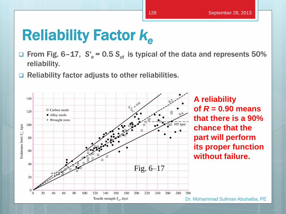
Reliability Factor ke From Fig. 6–17, S'e = 0.5 Sut is typical of the data and represents 50%
reliability.
Reliability factor adjusts to other reliabilities.
Dr. Mohammad Suliman Abuhaiba, PE
Fig. 6–17
September 28, 2013 128
A reliability
of R = 0.90 means
that there is a 90%
chance that the
part will perform
its proper function
without failure.
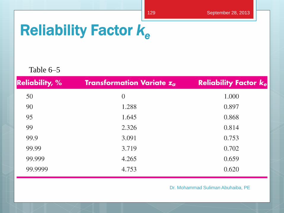
Reliability Factor ke
Dr. Mohammad Suliman Abuhaiba, PE
Table 6–5
September 28, 2013 129
Miscellaneous-Effects Factor kf
Consider other possible factors.
Residual stresses
Directional characteristics from cold working
Case hardening
Corrosion
Surface conditioning, e.g. electrolytic plating and metal
spraying
Cyclic Frequency
Frettage Corrosion
Limited data is available.
May require research or testing. Dr. Mohammad Suliman Abuhaiba, PE
September 28, 2013 130
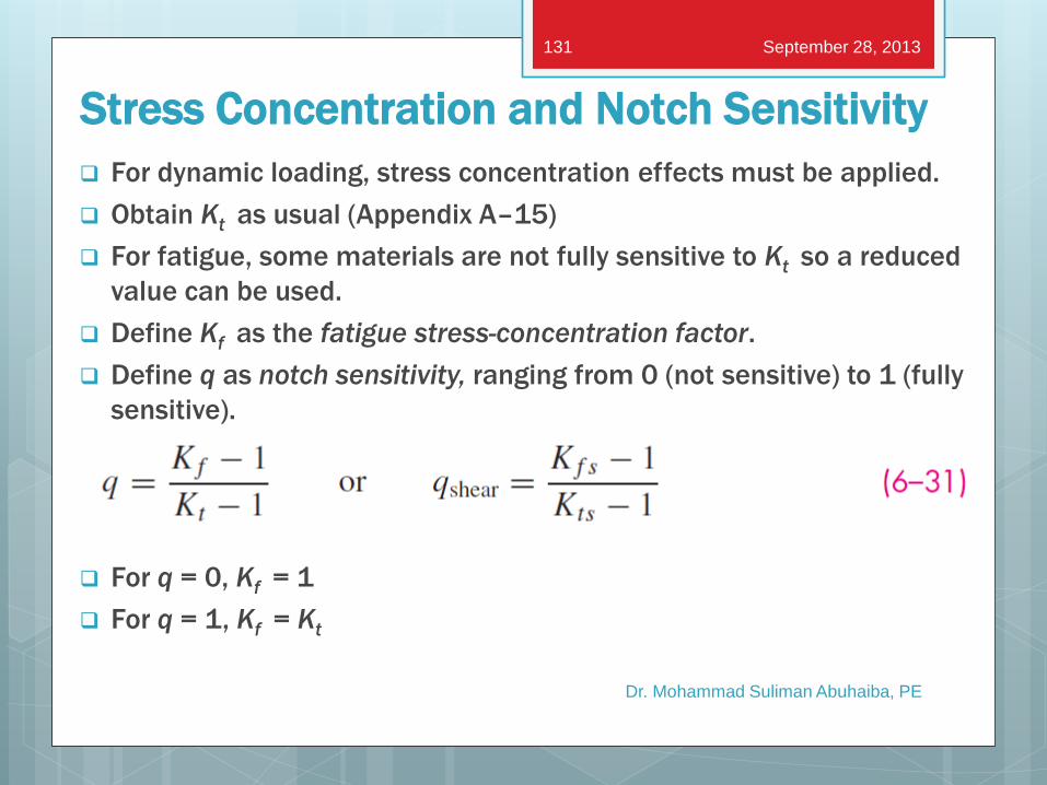
Stress Concentration and Notch Sensitivity
For dynamic loading, stress concentration effects must be applied.
Obtain Kt as usual (Appendix A–15)
For fatigue, some materials are not fully sensitive to Kt so a reduced
value can be used.
Define Kf as the fatigue stress-concentration factor.
Define q as notch sensitivity, ranging from 0 (not sensitive) to 1 (fully
sensitive).
For q = 0, Kf = 1
For q = 1, Kf = Kt
Dr. Mohammad Suliman Abuhaiba, PE
September 28, 2013 131
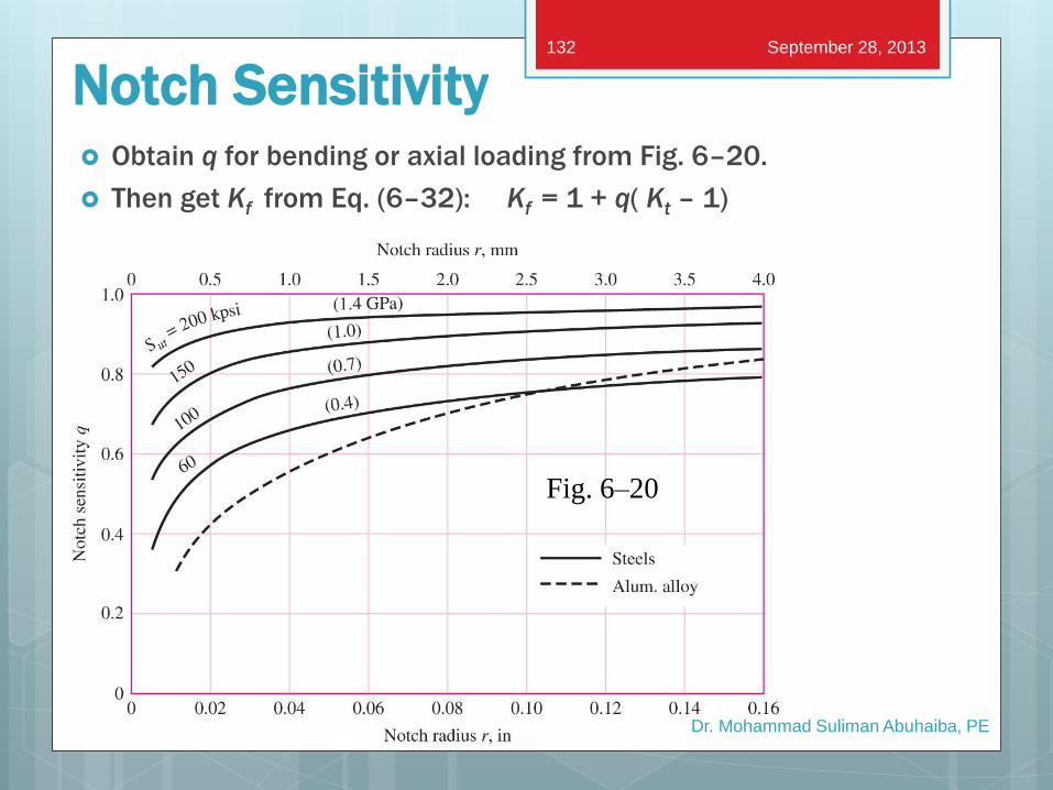
Notch Sensitivity Obtain q for bending or axial loading from Fig. 6–20.
Then get Kf from Eq. (6–32): Kf = 1 + q( Kt – 1)
Dr. Mohammad Suliman Abuhaiba, PE
Fig. 6–20
September 28, 2013 132
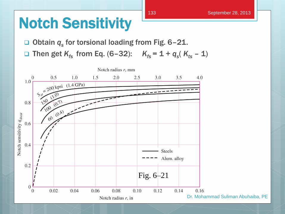
Notch Sensitivity Obtain qs for torsional loading from Fig. 6–21.
Then get Kfs from Eq. (6–32): Kfs = 1 + qs( Kts – 1)
Dr. Mohammad Suliman Abuhaiba, PE
Fig. 6–21
September 28, 2013 133
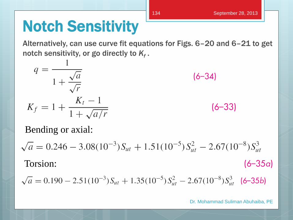
Notch Sensitivity Alternatively, can use curve fit equations for Figs. 6–20 and 6–21 to get
notch sensitivity, or go directly to Kf .
Dr. Mohammad Suliman Abuhaiba, PE
Bending or axial:
Torsion:
September 28, 2013 134
Notch Sensitivity for Cast Irons
Cast irons are already full of discontinuities, which are
included in the strengths.
Additional notches do not add much additional harm.
Recommended to use q = 0.2 for cast irons.
Dr. Mohammad Suliman Abuhaiba, PE
September 28, 2013 135
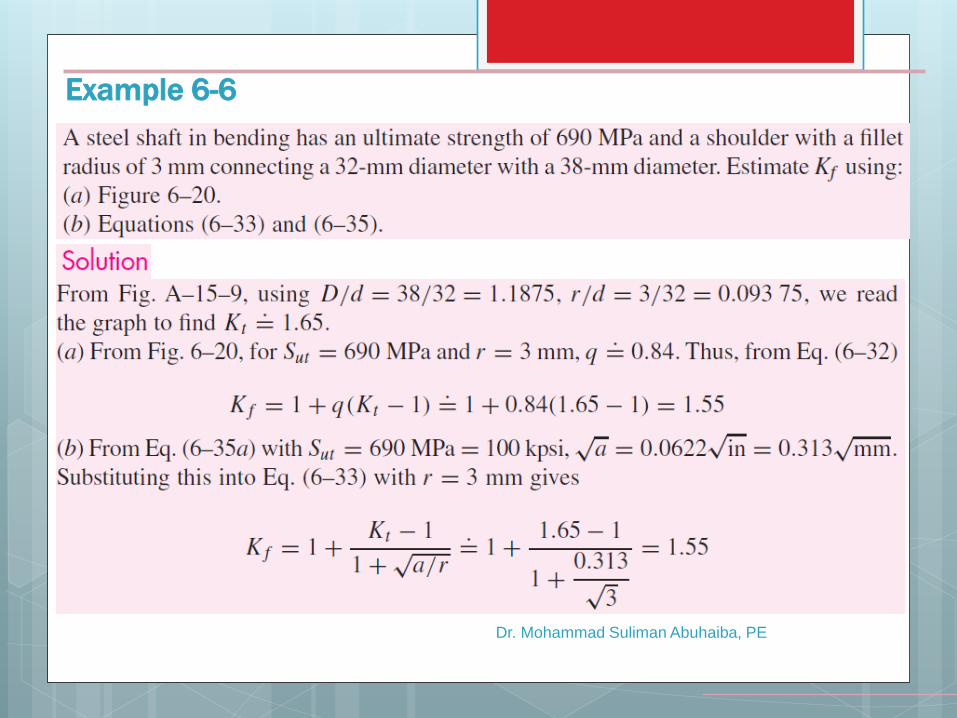
Example 6-6
Dr. Mohammad Suliman Abuhaiba, PE
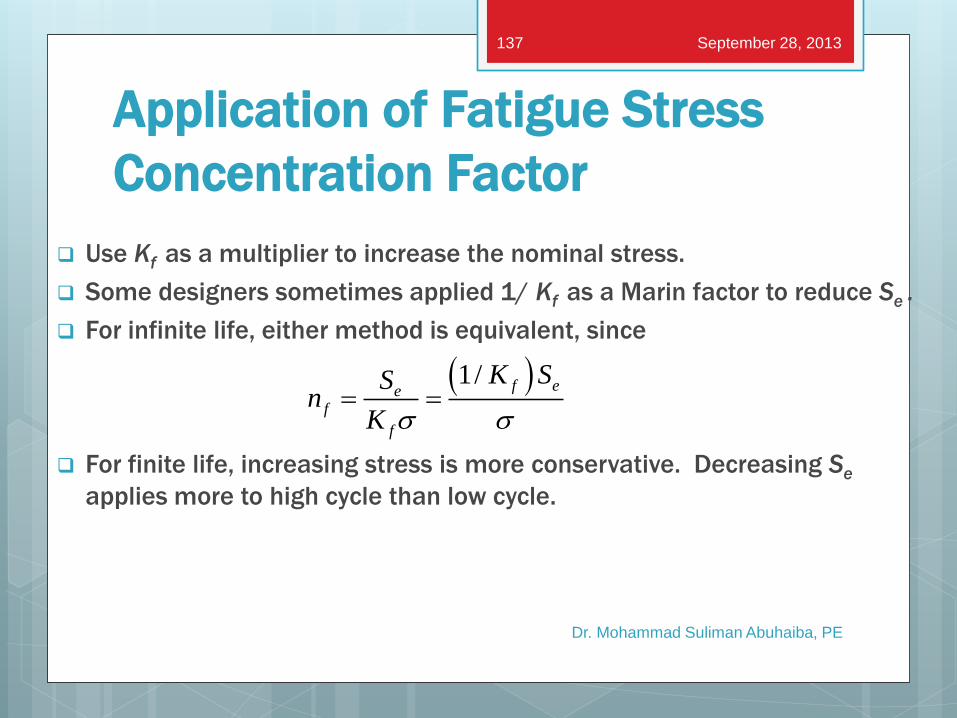
Application of Fatigue Stress
Concentration Factor
Use Kf as a multiplier to increase the nominal stress.
Some designers sometimes applied 1/ Kf as a Marin factor to reduce Se .
For infinite life, either method is equivalent, since
For finite life, increasing stress is more conservative. Decreasing Se
applies more to high cycle than low cycle.
Dr. Mohammad Suliman Abuhaiba, PE
1/ f eef
f
K SSn
K s s
September 28, 2013 137
Dr. Mohammad Suliman Abuhaiba, PE
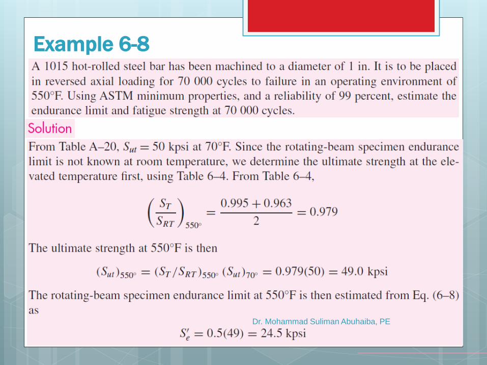
Example 6-8
Dr. Mohammad Suliman Abuhaiba, PE
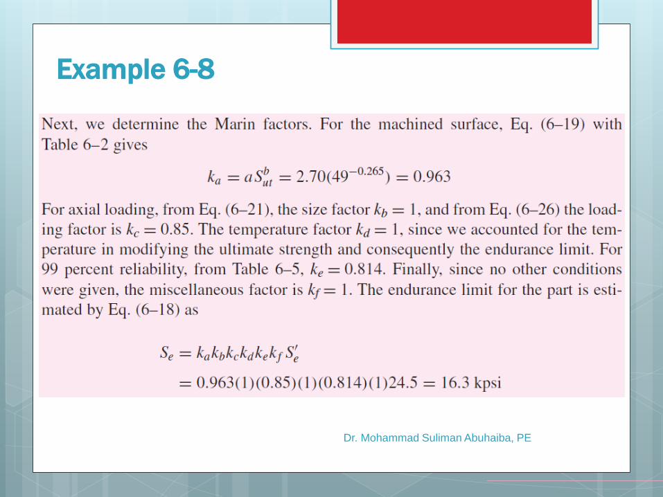
Example 6-8

Dr. Mohammad Suliman Abuhaiba, PE
Example 6-8
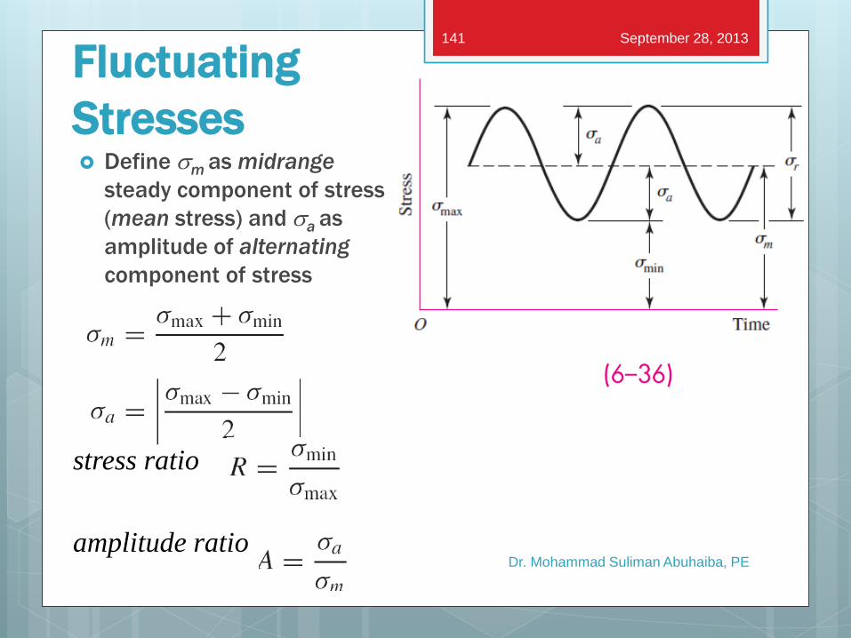
Fluctuating
Stresses Define sm as midrange
steady component of stress
(mean stress) and sa as
amplitude of alternating
component of stress
Dr. Mohammad Suliman Abuhaiba, PE
stress ratio
amplitude ratio
September 28, 2013 141
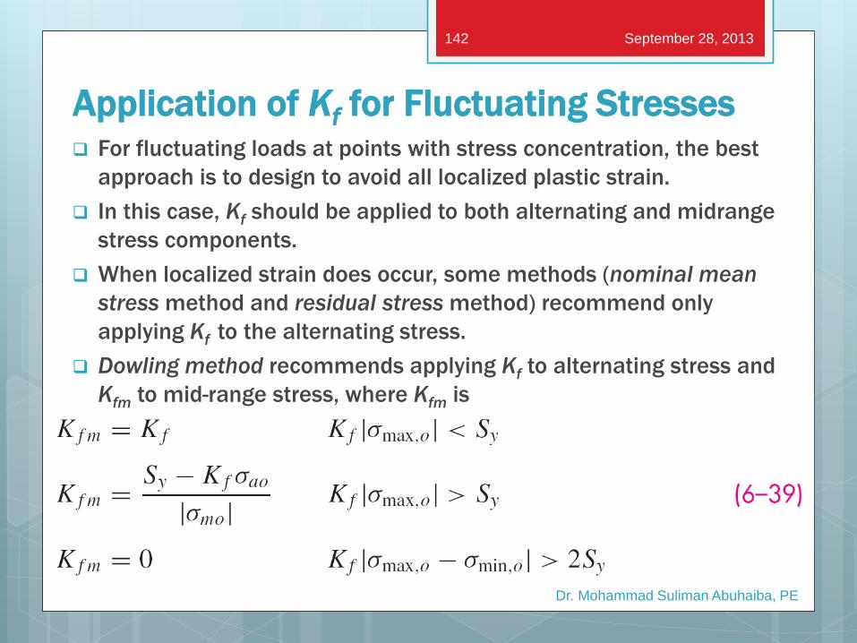
Application of Kf for Fluctuating Stresses For fluctuating loads at points with stress concentration, the best
approach is to design to avoid all localized plastic strain.
In this case, Kf should be applied to both alternating and midrange
stress components.
When localized strain does occur, some methods (nominal mean
stress method and residual stress method) recommend only
applying Kf to the alternating stress.
Dowling method recommends applying Kf to alternating stress and
Kfm to mid-range stress, where Kfm is
Dr. Mohammad Suliman Abuhaiba, PE
September 28, 2013 142
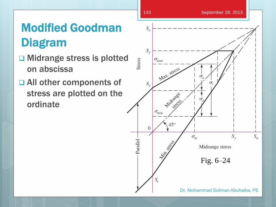
Modified Goodman
Diagram
Midrange stress is plotted
on abscissa
All other components of
stress are plotted on the
ordinate
Dr. Mohammad Suliman Abuhaiba, PE
Fig. 6–24
September 28, 2013 143
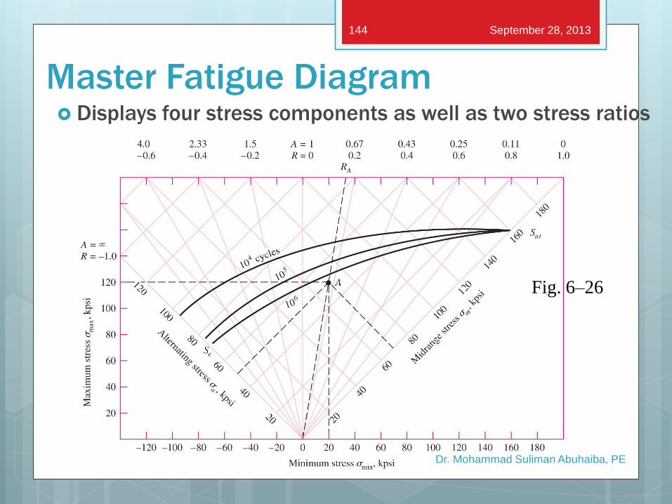
Master Fatigue Diagram Displays four stress components as well as two stress ratios
Dr. Mohammad Suliman Abuhaiba, PE
Fig. 6–26
September 28, 2013 144
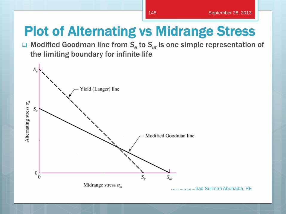
Plot of Alternating vs Midrange Stress Modified Goodman line from Se to Sut is one simple representation of
the limiting boundary for infinite life
Dr. Mohammad Suliman Abuhaiba, PE
September 28, 2013 145
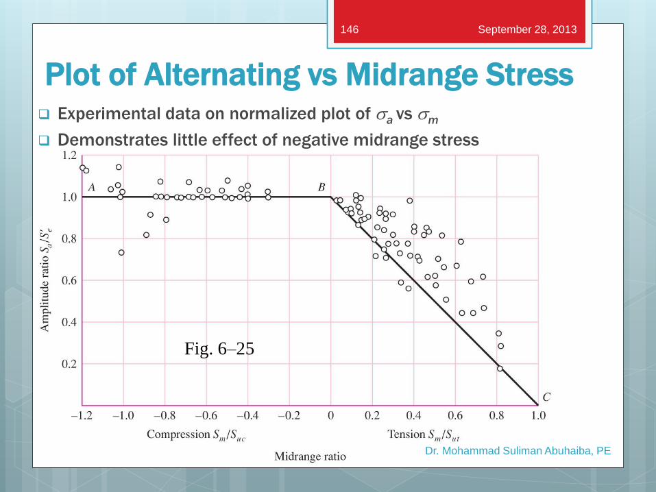
Plot of Alternating vs Midrange Stress Experimental data on normalized plot of sa vs sm
Demonstrates little effect of negative midrange stress
Dr. Mohammad Suliman Abuhaiba, PE
Fig. 6–25
September 28, 2013 146
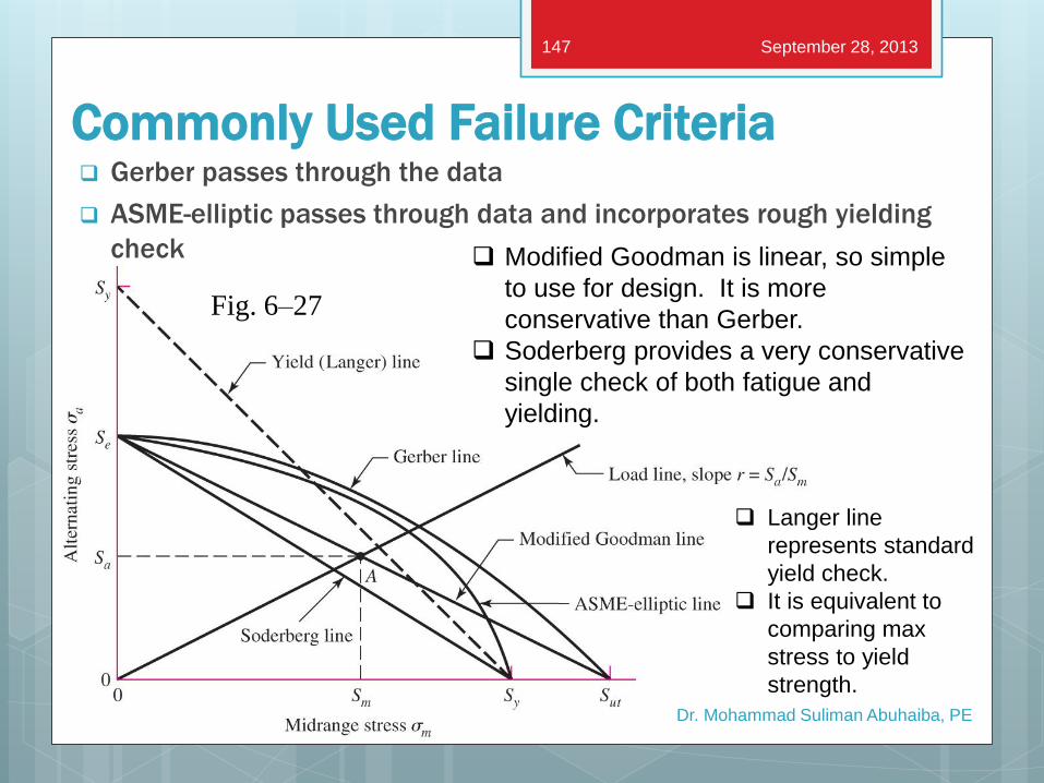
Commonly Used Failure Criteria Gerber passes through the data
ASME-elliptic passes through data and incorporates rough yielding
check
Dr. Mohammad Suliman Abuhaiba, PE
Fig. 6–27
September 28, 2013 147
Modified Goodman is linear, so simple
to use for design. It is more
conservative than Gerber.
Soderberg provides a very conservative
single check of both fatigue and
yielding.
Langer line
represents standard
yield check.
It is equivalent to
comparing max
stress to yield
strength.
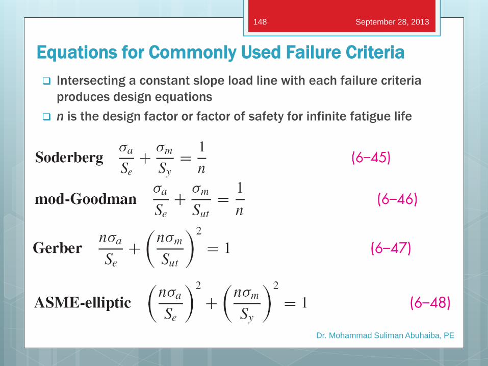
Equations for Commonly Used Failure Criteria
Intersecting a constant slope load line with each failure criteria
produces design equations
n is the design factor or factor of safety for infinite fatigue life
Dr. Mohammad Suliman Abuhaiba, PE
September 28, 2013 148
Summarizing Tables for Failure
Criteria Tables 6–6 to 6–8 summarize the pertinent equations for Modified
Goodman, Gerber, ASME-elliptic, and Langer failure criteria
The first row gives fatigue criterion
The second row gives yield criterion
The third row gives the intersection of static and fatigue criteria
The fourth row gives the equation for fatigue factor of safety
The first column gives the intersecting equations
The second column gives the coordinates of the intersection
Dr. Mohammad Suliman Abuhaiba, PE
September 28, 2013 149
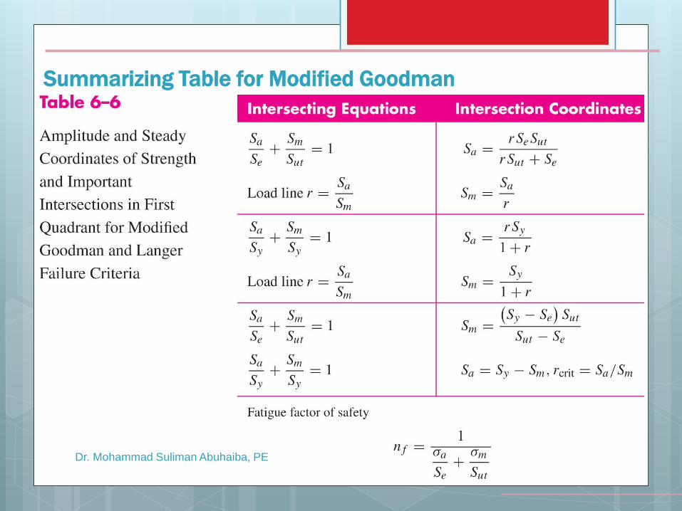
Summarizing Table for Modified Goodman
Dr. Mohammad Suliman Abuhaiba, PE
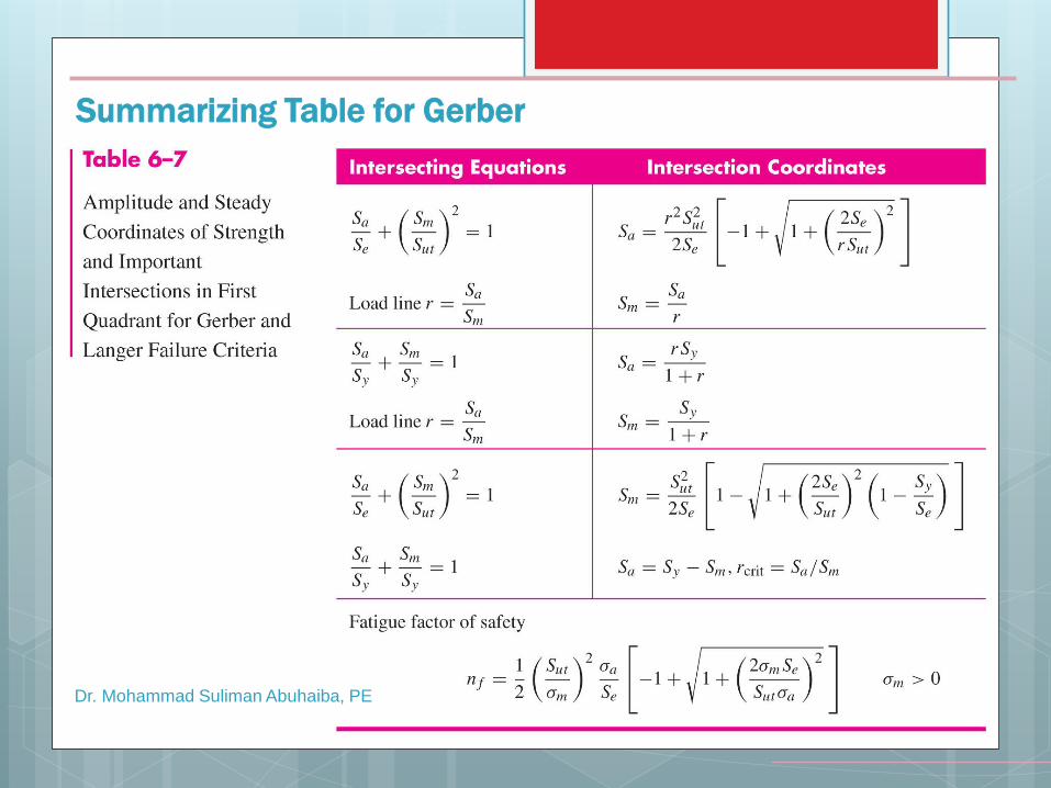
Summarizing Table for Gerber
Dr. Mohammad Suliman Abuhaiba, PE
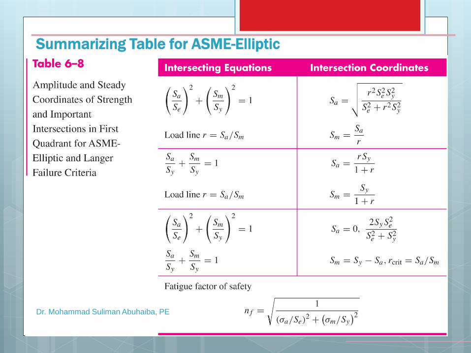
Summarizing Table for ASME-Elliptic
Dr. Mohammad Suliman Abuhaiba, PE
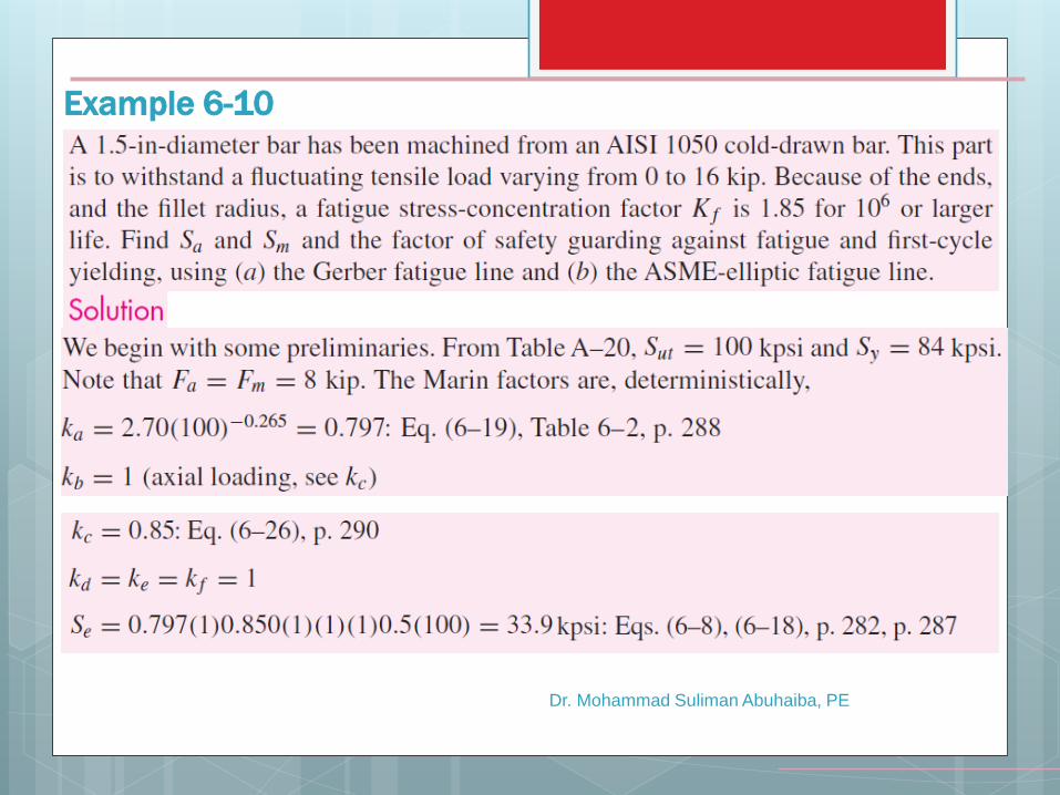
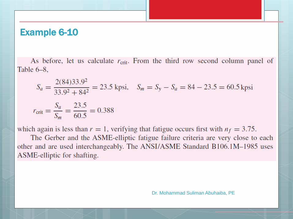
Example 6-10
Dr. Mohammad Suliman Abuhaiba, PE
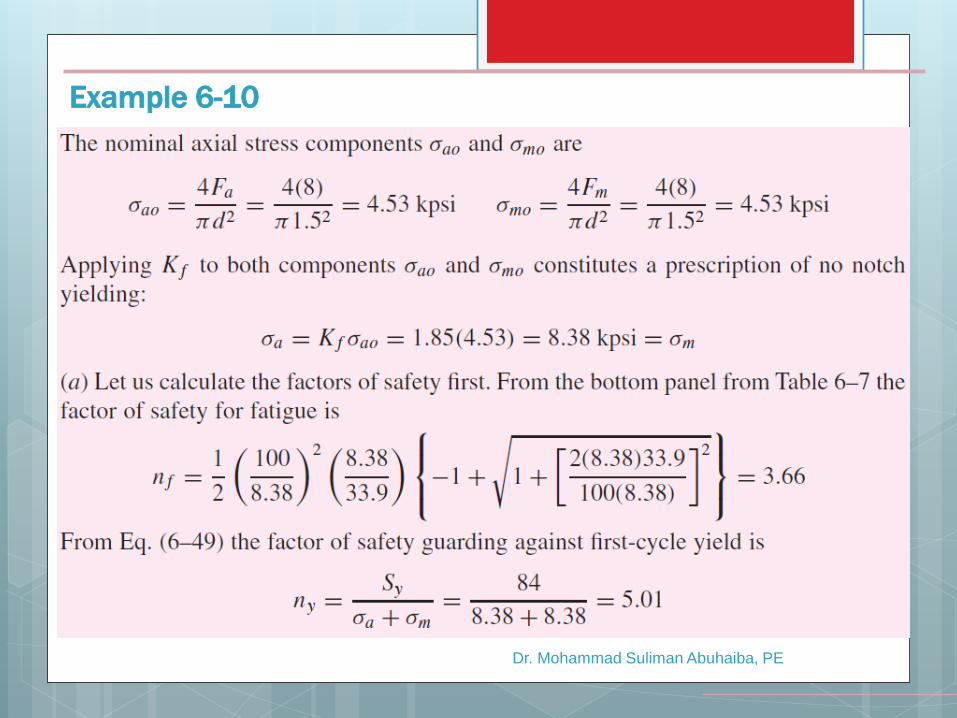
Example 6-10
Dr. Mohammad Suliman Abuhaiba, PE
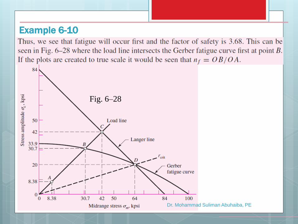
Example 6-10
Dr. Mohammad Suliman Abuhaiba, PE
Fig. 6–28
Example 6-10
Dr. Mohammad Suliman Abuhaiba, PE
Fig. 6–28

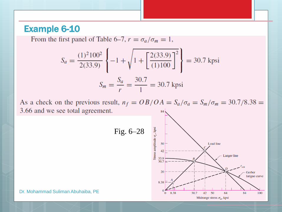
Example 6-10
Dr. Mohammad Suliman Abuhaiba, PE
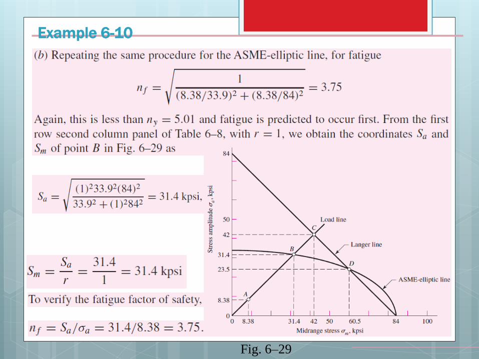
Example 6-10
Dr. Mohammad Suliman Abuhaiba, PE
Fig. 6–29
Example 6-10
Dr. Mohammad Suliman Abuhaiba, PE
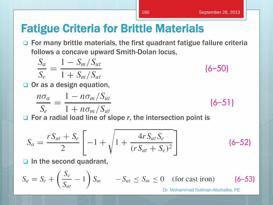
Fatigue Criteria for Brittle Materials For many brittle materials, the first quadrant fatigue failure criteria
follows a concave upward Smith-Dolan locus,
Or as a design equation,
For a radial load line of slope r, the intersection point is
In the second quadrant,
Dr. Mohammad Suliman Abuhaiba, PE
September 28, 2013 160
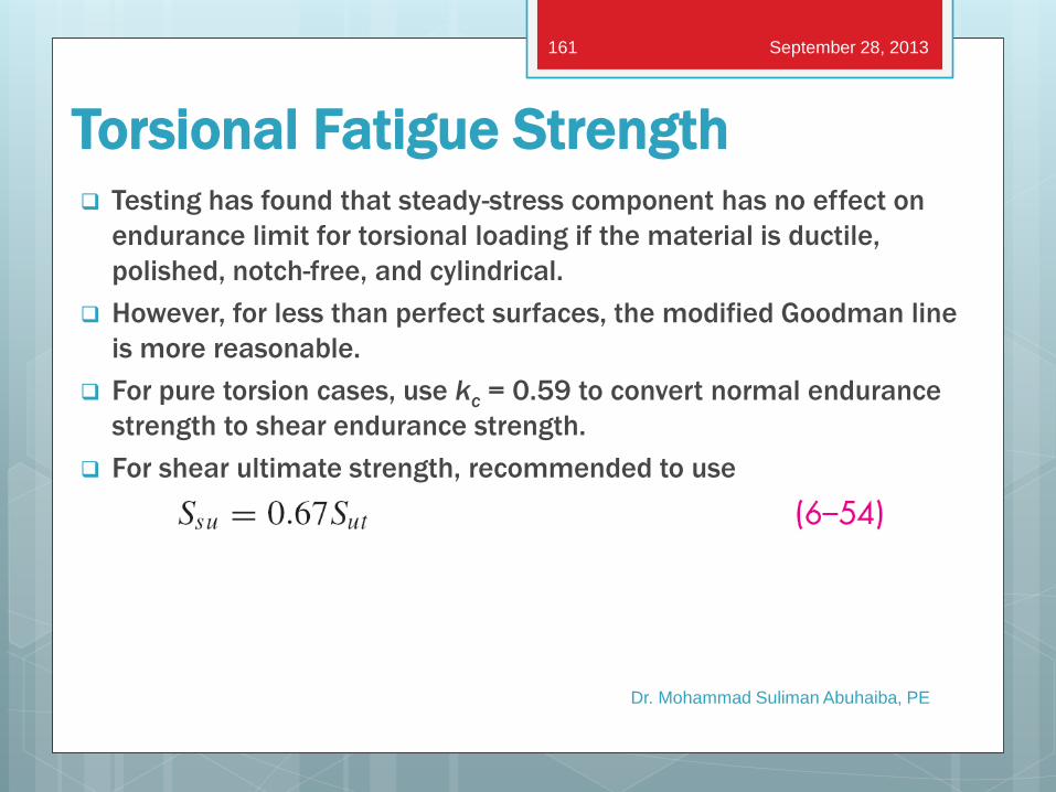
Torsional Fatigue Strength Testing has found that steady-stress component has no effect on
endurance limit for torsional loading if the material is ductile,
polished, notch-free, and cylindrical.
However, for less than perfect surfaces, the modified Goodman line
is more reasonable.
For pure torsion cases, use kc = 0.59 to convert normal endurance
strength to shear endurance strength.
For shear ultimate strength, recommended to use
Dr. Mohammad Suliman Abuhaiba, PE
September 28, 2013 161
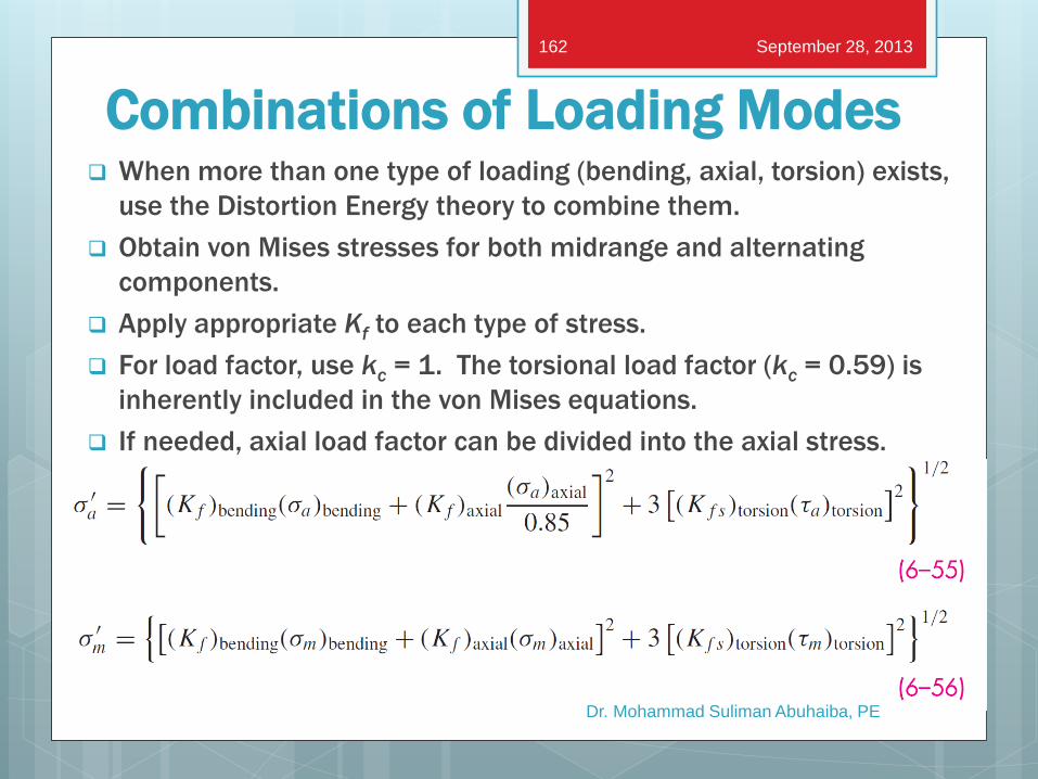
Combinations of Loading Modes When more than one type of loading (bending, axial, torsion) exists,
use the Distortion Energy theory to combine them.
Obtain von Mises stresses for both midrange and alternating
components.
Apply appropriate Kf to each type of stress.
For load factor, use kc = 1. The torsional load factor (kc = 0.59) is
inherently included in the von Mises equations.
If needed, axial load factor can be divided into the axial stress.
Dr. Mohammad Suliman Abuhaiba, PE
September 28, 2013 162
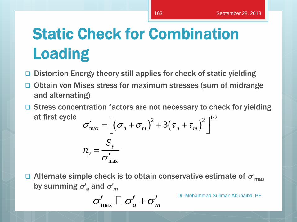
Static Check for Combination
Loading Distortion Energy theory still applies for check of static yielding
Obtain von Mises stress for maximum stresses (sum of midrange
and alternating)
Stress concentration factors are not necessary to check for yielding
at first cycle
Alternate simple check is to obtain conservative estimate of s'max
by summing s'a and s'm Dr. Mohammad Suliman Abuhaiba, PE
1/2
2 2
max
max
3a m a m
y
y
Sn
s s s t t
s
max a ms s s
September 28, 2013 163


![Best Practices In Load And Stress Testing Cmg Seminar[1]](https://img.pdfslide.us/doc/110x75/546998f0af7959e3018b6f6a/best-practices-in-load-and-stress-testing-cmg-seminar1.jpg)