Embed Size (px)
Citation preview
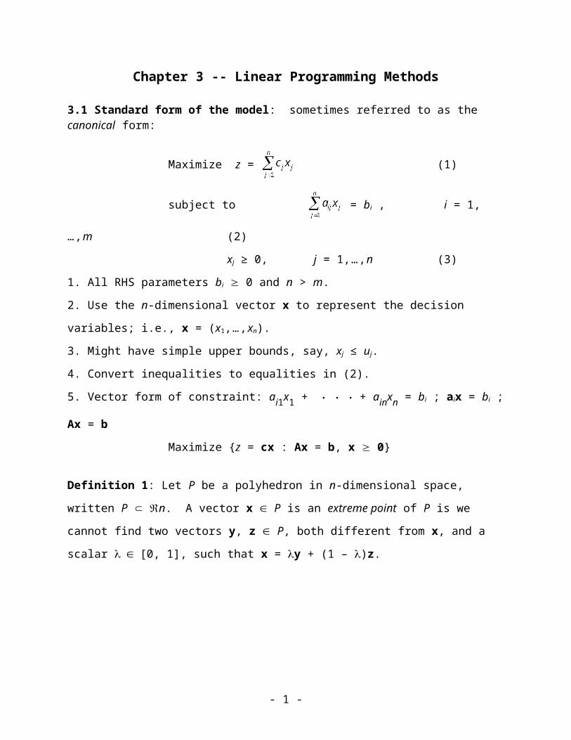
Chapter 3 -- Linear Programming Methods
3.1 Standard form of the model: sometimes referred to as the canonical form:
Maximize z = (1)
subject to = bi , i = 1,…,m (2)
xj ≥ 0, j = 1,…,n (3)
1. All RHS parameters bi 0 and n > m.
2. Use the n-dimensional vector x to represent the decision variables; i.e., x = (x1,…,xn).
3. Might have simple upper bounds, say, xj ≤ uj.
4. Convert inequalities to equalities in (2).
5. Vector form of constraint: ai1x1 + • • • + ainxn = bi ; aix = bi ; Ax = b
Maximize {z = cx : Ax = b, x 0}
Definition 1: Let P be a polyhedron in n-dimensional space, written P n. A vector x P is
an extreme point of P is we cannot find two vectors y, z P, both different from x, and a scalar
[0, 1], such that x = y + (1 – )z.
xyz
wu
v
P
••
•
•••
Figure 1. Some points in a polyhedron
Definition 2: Let a be a nonzero row vector in n-dimensional space, written a n, and let b be a scalar.
(a) The set {x n : ax = b} is called a hyperplane.(b) The set {x n : ax ≥ b} is called a halfspace.
- 1 -
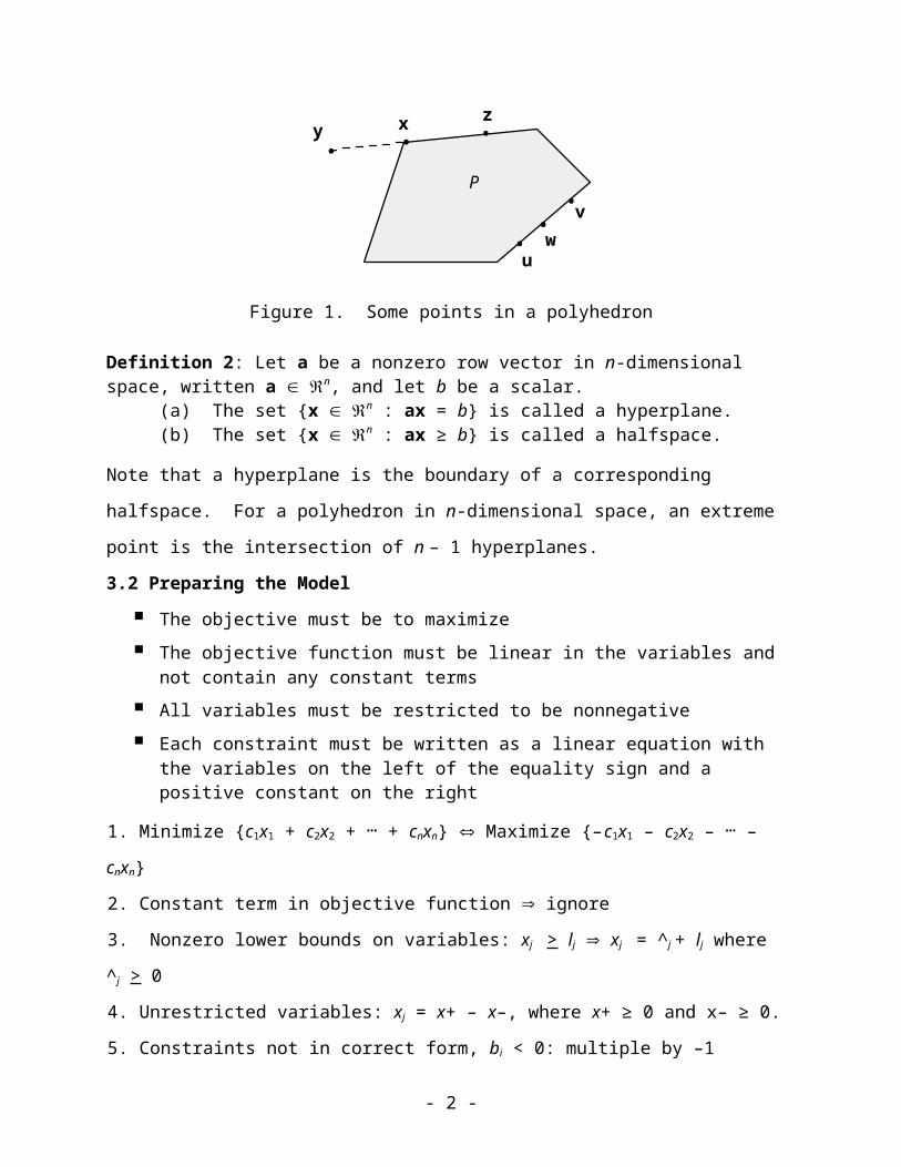
Note that a hyperplane is the boundary of a corresponding halfspace. For a polyhedron in n-
dimensional space, an extreme point is the intersection of n – 1 hyperplanes.
3.2 Preparing the Model
The objective must be to maximize
The objective function must be linear in the variables and not contain any constant terms
All variables must be restricted to be nonnegative
Each constraint must be written as a linear equation with the variables on the left of the equality sign and a positive constant on the right
1. Minimize {c1x1 + c2x2 + … + cnxn} Maximize {–c1x1 – c2x2 – … – cnxn}
2. Constant term in objective function ignore
3. Nonzero lower bounds on variables: xj > lj xj = ^j + lj where ^j > 0
4. Unrestricted variables: xj = x+ – x–, where x+ ≥ 0 and x– ≥ 0.
5. Constraints not in correct form, bi < 0: multiple by –1
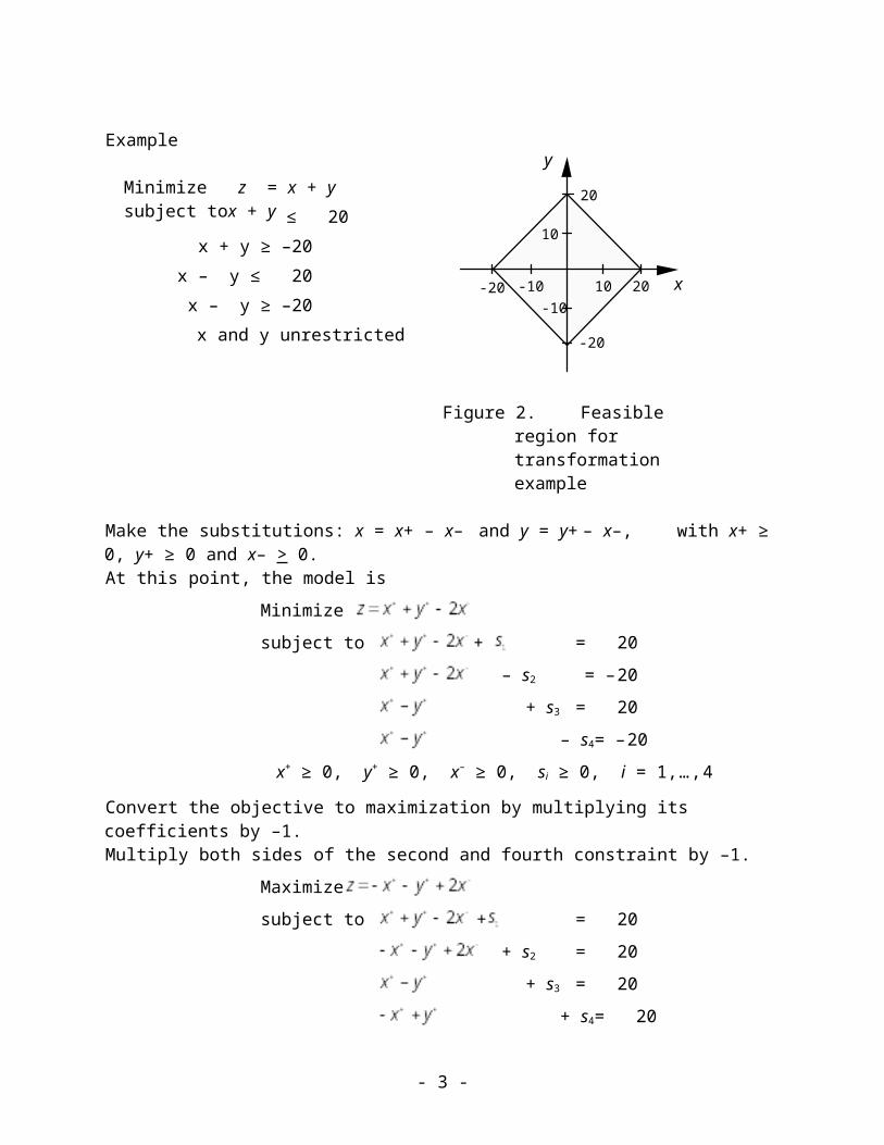
Example
Minimize z = x + ysubject to x + y ≤ 20
x + y ≥ –20x – y ≤ 20x – y ≥ –20
x and y unrestricted10 20-10-20 x
y
10
20
-20
-10
Figure 2. Feasible region for transformation example
Make the substitutions: x = x+ – x– and y = y+ – x–, with x+ ≥ 0, y+ ≥ 0 and x– > 0.At this point, the model is
Minimize
subject to + = 20
– s2 = –20
+ s3 = 20
– s4 = –20
- 2 -
x+ ≥ 0, y+ ≥ 0, x– ≥ 0, si ≥ 0, i = 1,…,4
Convert the objective to maximization by multiplying its coefficients by –1. Multiply both sides of the second and fourth constraint by –1.
Maximize
subject to + = 20
+ s2 = 20
+ s3 = 20
+ s4 = 20
x+ ≥ 0, y+ ≥ 0, x– ≥ 0, si ≥ 0, i = 1,…,4
Solution: x– = 10, s1 = 40, s3 = 20, s4 = 20, z = 20 x = –10, y = –10, z = – 20
Note that this problem has alternate optima. Any point on the line x + y = –20 yields the
objective value z = –20.
3.3 Geometric Properties of Linear Programs
Linear Independence: Let us consider a system of m linear equations in m unknowns:
a11x1 + a12x2 + • • • + a1mxm = b1
a21x1 + a22x2 + • • • + a2mxm = b2
am1x1 + am2x2 + • • • + ammxm = bm
1. Using vector notation, Ax = b, where A is an m m matrix and b is an m-dimensional column
vector.
2. For this system to have a unique solution, the matrix A must be invertible or nonsingular.
3. Must exist another m m matrix D such that AD = DA = I, where I is the m m identity
4. Matrix D is called the inverse of A and is unique. It is denoted by A–1.
Definition 3: Let A1,…,Ak be a collection of k column vectors, each of dimension m. We say that these vectors are linearly independent if it is not possible to find k real numbers 1, 2,…,k
not all zero such that jAj = 0, where 0 is the k-dimensional null vector; otherwise, they are called linearly dependent.
Equivalent definition
- 3 -
Theorem 1: Let A be a square matrix. The following statements are equivalent.
a. The matrix A is invertible as is its transpose AT.
b. The determinant of A is nonzero.
c. The rows and columns of A are linearly independent.
d. For every vector b, the linear system Ax = b has a unique solution.
Assuming that A–1 exists, a popular approach to solving the system Ax = b and thus obtaining the unique solution x = A–1b is Gauss-Jordan elimination. The simplex algorithm is based on this approach.
Basic Solutions: Let the matrix B = (A1,A2,…,Am) be nonsingular. Then we can uniquely solve
the equations
BxB = b
for the m-dimensional vector xB = (x1,…,xm). By putting x = (xB, 0), that is, by setting the first m components of x to those of xB and the remaining n – m components to zero, we obtain a solution to Ax = b. This leads to the following definition.
Definition 4: Given a set of m simultaneous linear equations (2) in n unknowns, let B be any
nonsingular m m matrix made up of columns of A. If all the n – m components of x not
associated with columns of B are set equal to zero, the solution to the resulting set of equations is
said to be a basic solution to (2) with respect to the basis B. The components of x associated
with columns of B are called basic variables.
Definition 5: A degenerate basic solution is said to occur if one or more of the basic variables
in a basic solution has value zero.
Definition 6: A vector x S = {x n : Ax = b, x ≥ 0} is said to be feasible to the linear
programming problem in standard form; a feasible solution that is also basic is said to be a basic
feasible solution (BFS). If this solution is degenerate, it is called a degenerate basic feasible
solution.
Foundations: We establish the relationship between optimality and basic feasible solutions in
the fundamental theorem of linear programming. The results tell us that when seeking a solution
to an LP it is only necessary to consider basic feasible solutions.
- 4 -
Theorem 2: Given a linear program in standard form (1) – (3) where A is an m n matrix of
rank m,
(i) if there is a feasible solution, there is a basic feasible solution;
(ii) if there is an optimal feasible solution, there is an optimal basic feasible solution.
Number of bases: = (4)
Many not feasible.
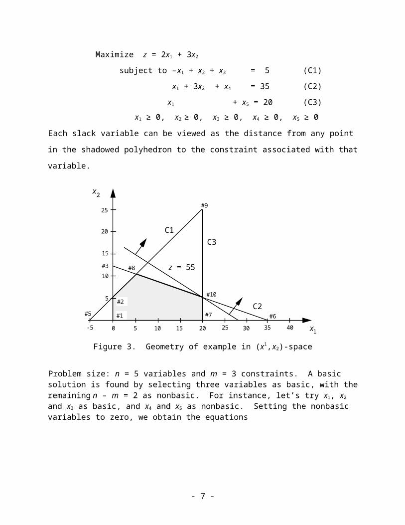
Example: Consider following linear program in standard form where slacks x3, x4, x5 have been added to the 3 constraints.
Maximize z = 2x1 + 3x2
subject to –x1 + x2 + x3 = 5 (C1)
x1 + 3x2 + x4 = 35 (C2)
x1 + x5 = 20 (C3)
x1 ≥ 0, x2 ≥ 0, x3 ≥ 0, x4 ≥ 0, x5 ≥ 0
Each slack variable can be viewed as the distance from any point in the shadowed polyhedron to
the constraint associated with that variable.
#8
0 5 1510 20 25 30 35 40 x
x2
1
5
10
15
20
25
-5
C1
C2
C3
#1
#2
#3
#5 #6#7
#9
#10
z = 55
Figure 3. Geometry of example in (x1,x2)-space
- 5 -
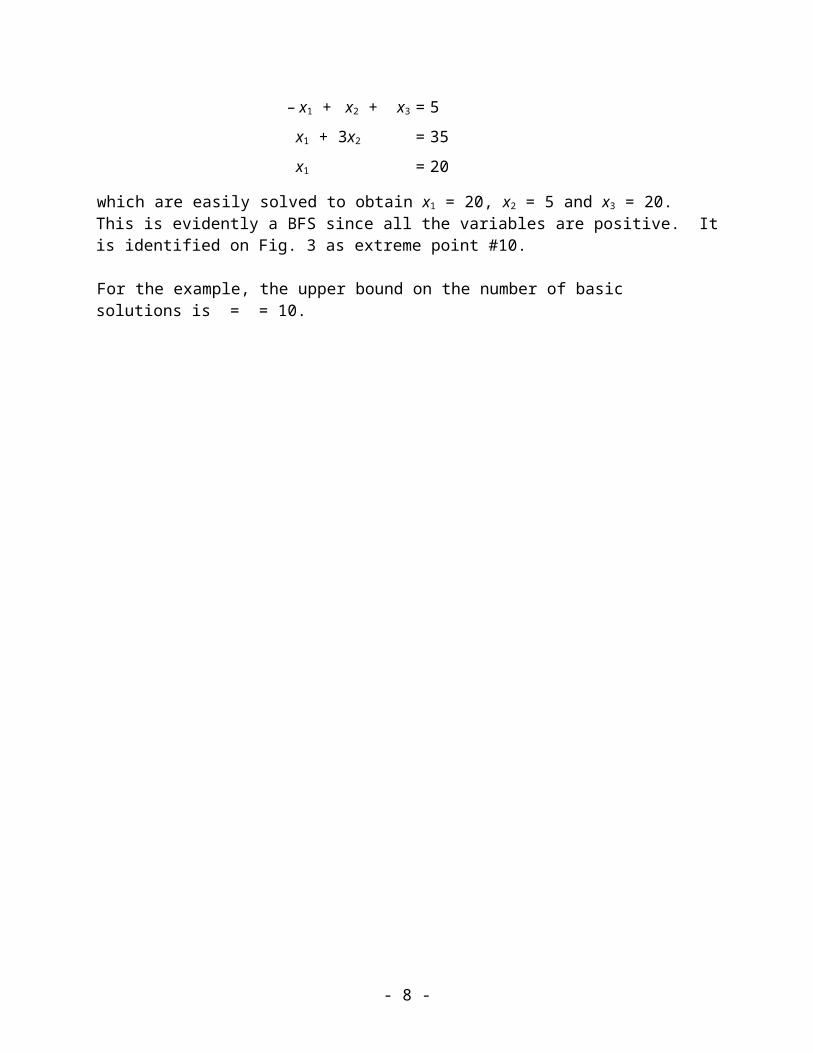
Problem size: n = 5 variables and m = 3 constraints. A basic solution is found by selecting three variables as basic, with the remaining n – m = 2 as nonbasic. For instance, let’s try x1, x2 and x3 as basic, and x4 and x5 as nonbasic. Setting the nonbasic variables to zero, we obtain the equa-tions
– x1 + x2 + x3 = 5
x1 + 3x2 = 35
x1 = 20
which are easily solved to obtain x1 = 20, x2 = 5 and x3 = 20. This is evidently a BFS since all the variables are positive. It is identified on Fig. 3 as extreme point #10.
For the example, the upper bound on the number of basic solutions is = = 10.
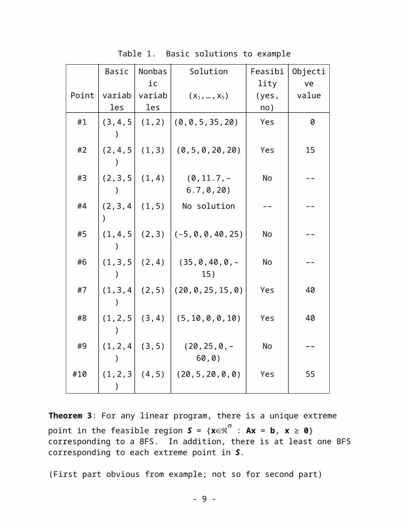
Table 1. Basic solutions to example
Basic Nonbasic Solution Feasibility ObjectivePoint variables variables (x1,…,x5) (yes, no) value
#1 (3,4,5) (1,2) (0,0,5,35,20) Yes 0
#2 (2,4,5) (1,3) (0,5,0,20,20) Yes 15
#3 (2,3,5) (1,4) (0,11.7,–6.7,0,20) No ––
#4 (2,3,4) (1,5) No solution –– ––
#5 (1,4,5) (2,3) (–5,0,0,40,25) No ––
#6 (1,3,5) (2,4) (35,0,40,0,–15) No ––
#7 (1,3,4) (2,5) (20,0,25,15,0) Yes 40
#8 (1,2,5) (3,4) (5,10,0,0,10) Yes 40
#9 (1,2,4) (3,5) (20,25,0,–60,0) No ––
#10 (1,2,3) (4,5) (20,5,20,0,0) Yes 55
Theorem 3: For any linear program, there is a unique extreme point in the feasible region S = {xn : Ax = b, x ≥ 0} corresponding to a BFS. In addition, there is at least one BFS corresponding to each extreme point in S.
(First part obvious from example; not so for second part)
Definition 7: For a linear program in standard form with m constraints, two basic feasible solutions are said to be adjacent if they have m – 1 basic variables in common.
- 6 -
Theorem 4: For a linear program in standard form (1) – (3), let xl be a BFS and let E(l) be the
index set of all BFSs adjacent to xl. Define zl z(xl). If
zl ≥ zk for all k E(l)then xl is an optimal BFS.
Outline of Simplex Algorithm (max problem)
Step 1 Find an initial BFS to the linear program. As the algorithm progresses, the most recent
BFS will be called the incumbent.
Step 2 Determine if the incumbent is optimal. If so, stop; otherwise go to Step 3.
Step 3 Move to an adjacent BFS that has a larger z value and return to Step 2 using the new
BFS as the incumbent.
3.4 Simplex Tableau
Previous model in slightly modified form Simplex Form:
Maximize z
(E0) z – 2x1 – 3x2 = 0
(E1) –x1 + x2 + x3 = 5
(E2) x1 + 3x2 + x4 = 35
(E3) x1 + x5 = 20
xj ≥ 0, j = 1,…,5
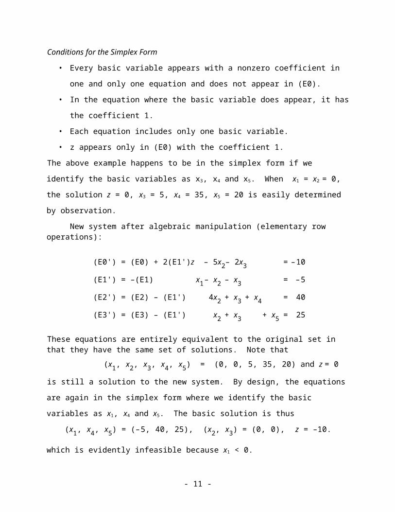
Conditions for the Simplex Form
• Every basic variable appears with a nonzero coefficient in one and only one equation and
does not appear in (E0).
• In the equation where the basic variable does appear, it has the coefficient 1.
• Each equation includes only one basic variable.
• z appears only in (E0) with the coefficient 1.
The above example happens to be in the simplex form if we identify the basic variables as x3, x4
and x5. When x1 = x2 = 0, the solution z = 0, x3 = 5, x4 = 35, x5 = 20 is easily determined by
observation.
New system after algebraic manipulation (elementary row operations):
- 7 -
(E0') = (E0) + 2(E1') z – 5x2 – 2x3 = –10
(E1') = –(E1) x1 – x2 – x3 = –5
(E2') = (E2) – (E1') 4x2 + x3 + x4 = 40
(E3') = (E3) – (E1') x2 + x3 + x5 = 25
These equations are entirely equivalent to the original set in that they have the same set of solutions. Note that
(x1, x2, x3, x4, x5) = (0, 0, 5, 35, 20) and z = 0
is still a solution to the new system. By design, the equations are again in the simplex form
where we identify the basic variables as x1, x4 and x5. The basic solution is thus
(x1, x4, x5) = (–5, 40, 25), (x2, x3) = (0, 0), z = –10.
which is evidently infeasible because x1 < 0.
General Simplex FormDuring the simplex computations, we will use -ij to denote the current coefficient of xj in
equation i, for i = 1,…,m and j = 1,…,n. We use -j in equation (E0) to denote the current value
of the jth objective function coefficient. For minimization objective values are known as
reduced costs or relative costs. They are the unit costs relative to the current set of nonbasic
variables in the reduced model in which the basic variables are fixed.
The general form of the model is
(E0) z + = -
(Ei) xB(i) + = -i, i = 1,…,m
The “bars” on the coefficients -ij, -i, -j indicate that these values are not in general the same as
those in the original model (1) – (3).
Tableau Description of Equations
To organize the computations, it is common to convert the algebraic model to a tableau, as illustrated in Table 2 for the example problem.
- 8 -
Algebraic Model
(E0) z – 2x1 – 3x2 = 0
(E1) –x1 + x2 + x3 = 5
(E2) x1 + 3x2 + x4 = 35
(E3) x1 + x5 = 20
Table 2. Tableau form of example problem, E(0) – E(3)
CoefficientsRow Basic RHS
0 1 –2 –3 0 0 0 01 0 –1 1 1 0 0 52 0 1 3 0 1 0 353 0 1 0 0 0 1 20
x1zz
x2 x3 x4 x5
x3
x4
x5
Table 3 gives the tableau for the updated set of equations (E0') - (E3').
Table 3. Tableau for equations (E0') – (E3')
CoefficientsRow Basic RHS
0 1 0 –5 –2 0 0 –101 0 1 –1 –1 0 0 –52 0 0 4 1 1 0 403 0 0 1 1 0 1 25
x1zz
x2 x3 x4 x5
x4
x5
x1
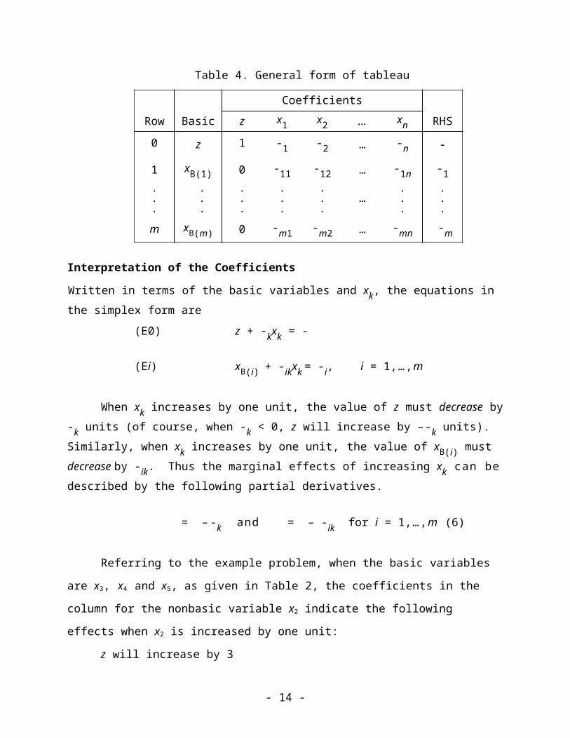
The tableau in Table 4 gives the general form for a problem with n variables and m constraints.
It is assumed that m variables have been singled out as basic.
- 9 -
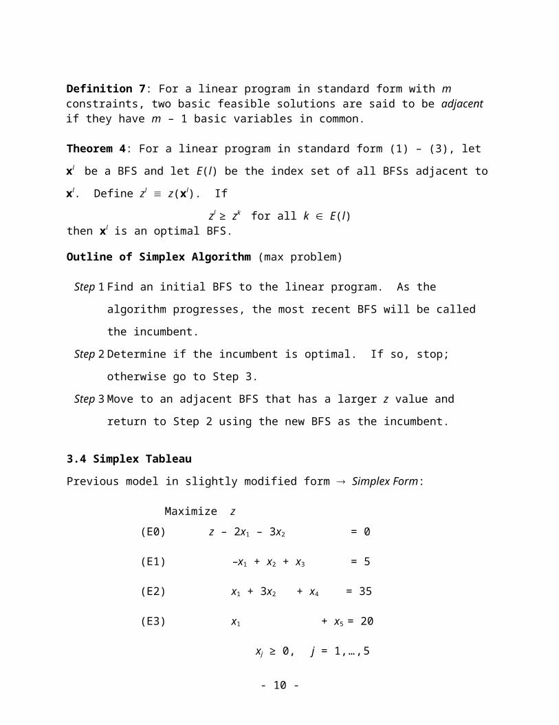
Table 4. General form of tableau
Coefficients
Row Basic z x1 x2 … xn RHS0 z 1 -1 -2 … -n -
1 xB(1) 0 -11 -12 … -1n -1...
.
.
.
.
.
.
.
.
.
.
.
.…
.
.
.
.
.
.
m xB(m) 0 -m1 -m2 … -mn-m
Interpretation of the Coefficients
Written in terms of the basic variables and xk, the equations in the simplex form are
(E0) z + -kxk = -
(Ei) xB(i) + -ikxk = -i, i = 1,…,m
When xk increases by one unit, the value of z must decrease by -k units (of course, when -
k < 0, z will increase by –-k units). Similarly, when xk increases by one unit, the value of xB(i) must decrease by -ik. Thus the marginal effects of increasing xk can be described by the following partial derivatives.
= – -k and = – -ik for i = 1,…,m (6)
Referring to the example problem, when the basic variables are x3, x4 and x5, as given in
Table 2, the coefficients in the column for the nonbasic variable x2 indicate the following effects
when x2 is increased by one unit:
z will increase by 3
x3 will decrease by 1
x4 will decrease by 3
x5 will not change.
- 10 -
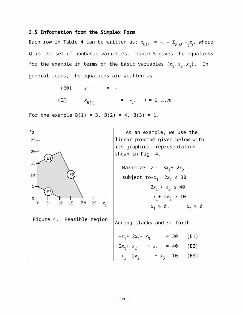
3.5 Information from the Simplex Form
Each row in Table 4 can be written as: xB(i) = -i – jQ -ijxj, where Q is the set of nonbasic
variables. Table 5 gives the equations for the example in terms of the basic variables (x1, x3, x4).
In general terms, the equations are written as
(E0) z + = -
(Ei) xB(i) + = -i, i = 1,…,m
For the example B(1) = 3, B(2) = 4, B(3) = 1.
x2
0
5
10
15
20
25
0 5 10 15 20 25
E3
E2
E1
x1
Figure 4. Feasible region
As an example, we use the linear program given below with its graphical representation shown in Fig. 4.
Maximize z = 3x1 + 2x2
subject to –x1 + 2x2 ≤ 30
2x1 + x2 ≤ 40
x1 + 2x2 ≥ 10
x1 ≥ 0, x2 ≥ 0
Adding slacks and so forth
–x1 + 2x2 + x3 = 30 (E1)
2x1 + x2 + x4 = 40 (E2)
–x1 – 2x2 + x5 = –10 (E3)
- 11 -
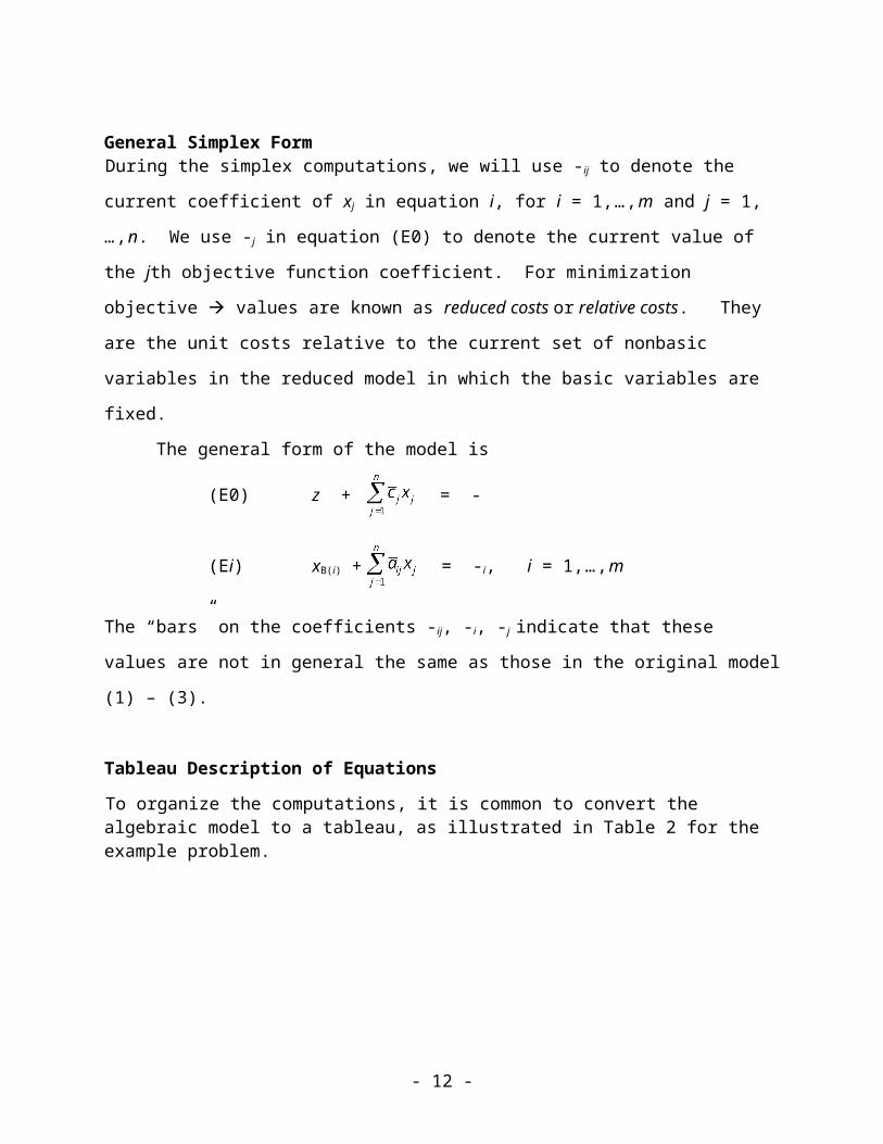
Table 5. Tableau corresponding to origin in Fig. 6
CoefficientsRow Basic z x1 x2 x3 x4 x5 RHS
0 z 1 0 4 0 0 –3 301 x3 0 0 4 1 0 –1 402 x4 0 0 –3 0 1 2 203 x1 0 1 2 0 0 –1 10
Solution from tableau: x = (10, 0, 40, 20, 0) with z = 30.
From the general expression of the simplex form we read the objective function value and the values of the basic variables as
z = -, xB(i) = -i for i = 1,…,m, and xj = 0 for j Q.
Is the basic solution feasible? -i ≥ 0 for i = 1,…,m?
Is the feasible basic solution optimal?
The objective function equation for the example is
(E0) z + 4x2 – 3x5 = 30
For the current BFS, both x2 and x5 are zero, so decreasing either causes the solution to become
infeasible. We therefore restrict attention to increases. When one of the nonbasic variables is
held at zero, only z and the other nonbasic variable play a role in (E0).
For x2 active, we have z = 30 – 4x2.
For x5 active, we have z = 30 + 3x5
We wish to increase x5 because we want to maximize the objective function.
Optimality conditions: -j ≥ 0 for all j Q
Condition easily tested by examining equation (E0) in the simplex form or row 0 of the tableau.
How can a nonoptimal feasible solution be improved? In the general case, all nonbasic
variables xj with -j < 0 are candidates to become basic.
- 12 -
How much should the nonbasic variable be changed?
From the example, when x2 is held at 0, we have
x3 = 40 + x5
x4 = 20 – 2x5
x1 = 10 + x5
As x5 –> 10, x4 –> 0 which determines how much the nonbasic variable x5 can change.
Minimum ratio test
= minimum
It is possible that no positive value of -ij exists for some nonbasic variable xk such that -k < 0. This implies that xk and z can be increased indefinitely without the solution becoming infeasible. When this occurs, there is no finite optimum so the solution is said to be unbounded.
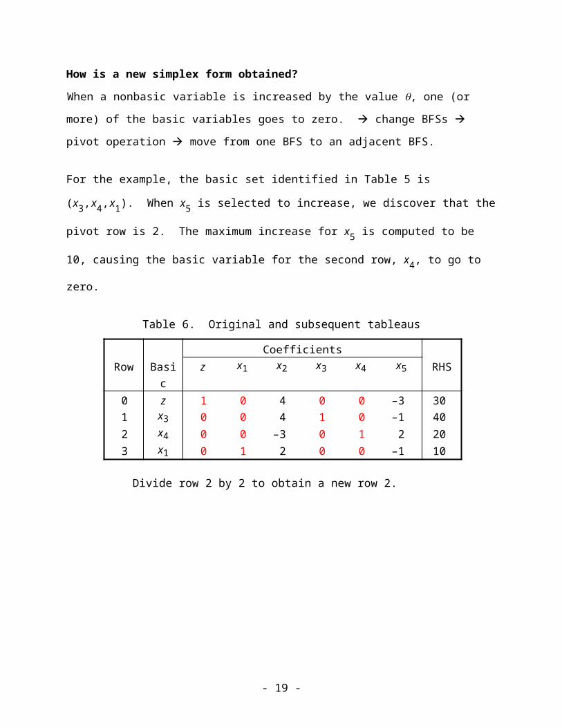
How is a new simplex form obtained?
When a nonbasic variable is increased by the value , one (or more) of the basic variables goes
to zero. change BFSs pivot operation move from one BFS to an adjacent BFS.
For the example, the basic set identified in Table 5 is (x3,x4,x1). When x5 is selected to increase,
we discover that the pivot row is 2. The maximum increase for x5 is computed to be 10, causing
the basic variable for the second row, x4, to go to zero.
Table 6. Original and subsequent tableaus
CoefficientsRow Basic z x1 x2 x3 x4 x5 RHS
0 z 1 0 4 0 0 –3 301 x3 0 0 4 1 0 –1 402 x4 0 0 –3 0 1 2 203 x1 0 1 2 0 0 –1 10
Divide row 2 by 2 to obtain a new row 2.
- 13 -
CoefficientsRow Basic z x1 x2 x3 x4 x5 RHS
0 z 1 0 4 0 0 –3 301 x3 0 0 4 1 0 –1 402 x5 0 0 –3/2 0 1/2 1 10
3 x1 0 1 2 0 0 –1 10
Multiply the new row 2 by +3 and add it to row 0,
Multiply the new row 2 by +1 and add it to row 1,
Multiply the new row 2 by +1 and add it to row 3,
to obtain:
CoefficientsRow Basic z x1 x2 x3 x4 x5 RHS
0 z 1 0 –1/2 0 3/2 0 601 x3 0 0 5/2 1 –1/2 0 502 x5 0 0 –3/2 0 1/2 1 103 x1 0 1 1/2 0 –1/2 0 20
The third tableau in Table 6 is in the simplex form for the basic variables (x3, x5, x1). The BFS is easily seen to be
x = (20, 0, 50, 0, 10) with z = 60.As expected, the objective value has improved by –-5 = –3 10 = 30 to a value of 60. We observe from row 0 that the solution is still not optimal.
Pivot operations: Let the variable entering the basis be xk and let the pivot row be r. Now,(i) divide row r by the pivot element -rk; (ii) for each row i, (i = 0,…,m, i ≠ r), multiply the new row r by –-ik and add it to row i.
- 14 -

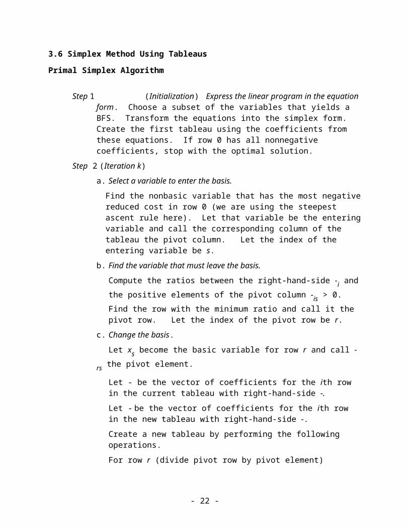
3.6 Simplex Method Using Tableaus
Primal Simplex Algorithm
Step 1 (Initialization) Express the linear program in the equation form. Choose a subset of the variables that yields a BFS. Transform the equations into the simplex form. Create the first tableau using the coefficients from these equations. If row 0 has all nonnegative coefficients, stop with the optimal solution.
Step 2 (Iteration k)
a. Select a variable to enter the basis.
Find the nonbasic variable that has the most negative reduced cost in row 0 (we are using the steepest ascent rule here). Let that variable be the entering vari-able and call the corresponding column of the tableau the pivot column. Let the index of the entering variable be s.
b. Find the variable that must leave the basis.
Compute the ratios between the right-hand-side -i and the positive elements of the pivot column -is > 0. Find the row with the minimum ratio and call it the pivot row. Let the index of the pivot row be r.
c. Change the basis.
Let xs become the basic variable for row r and call -rs the pivot element.
Let - be the vector of coefficients for the ith row in the current tableau with right-hand-side -.
Let - be the vector of coefficients for the ith row in the new tableau with right-hand-side -.
Create a new tableau by performing the following operations.
For row r (divide pivot row by pivot element)
- = - / -rs and - = - / -rs
For row i = 0,1,…,m and i ≠ r (multiply the new pivot row by the negative of the ith coefficient in the pivot column and add the result to row i)
- = (–- -) + - and - = (–- -) + -
Step 3 (Optimality test) If all reduced costs in row 0 are nonnegative, stop with the optimal solution. Otherwise return to Step 2.
- 15 -
Example
We will use as an example the problem considered in Section 3.4. The tableau in Table 2 is repeated in Table 7 with slacks x3, x4 and x5.
Table 7. Initial tableau for simplex example
CoefficientsRow Basic RHS
0 1 -2 -3 0 0 0 01 0 -1 1 1 0 0 52 0 1 3 0 1 0 353 0 1 0 0 0 1 20
x1zz
x2 x3 x4 x5
x 3
x 4
x 5
Step 1 (Initialization)
Note that the initial tableau is in the simplex form. Choosing the slacks x3, x4, x5 as the basic variables gives a BFS. This is a direct result of the original model having all (≤) constraints and positive constants on the right-hand side. In cases such as this, the slack variables will always define a BFS and provide a convenient starting basis for the simplex method. Thus the initialization step is accomplished for the example. From row 0 we see that the solution is not optimal.
Iteration 1
Step 2 (Iterate - update tableau)
a Using the most negative rule, we choose x2 as the entering variable (s = 2).
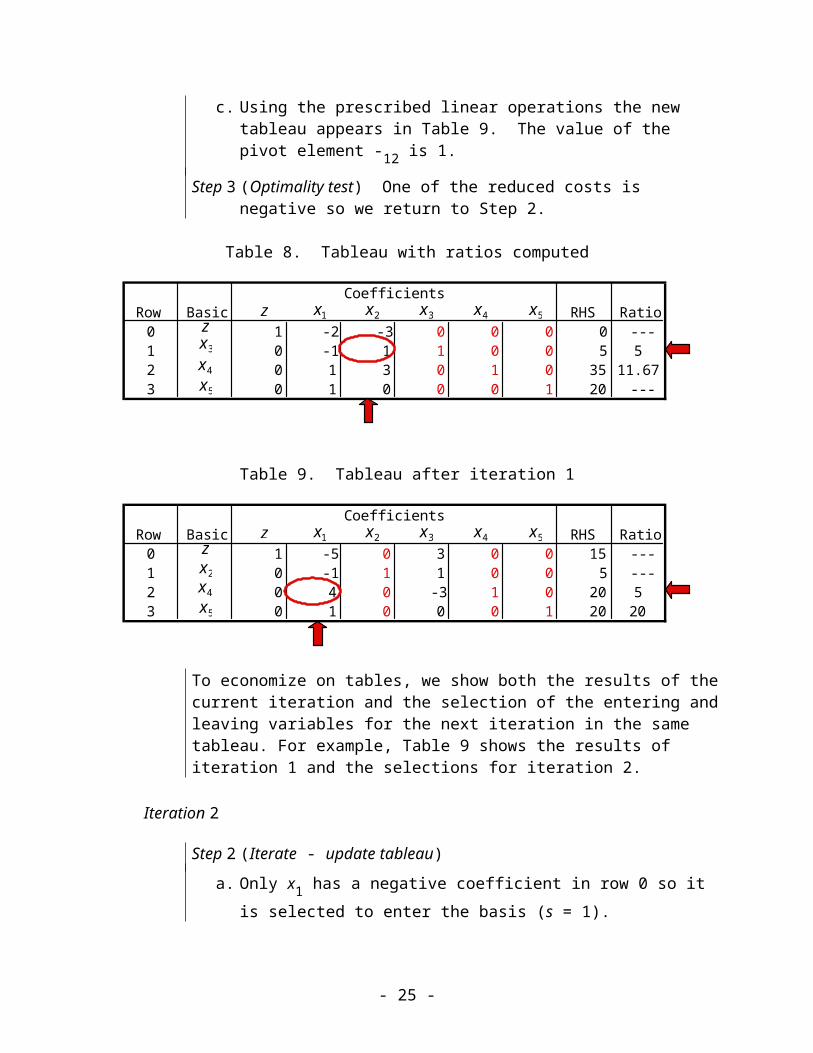
b. We compute the ratios -i / -is for positive -is. For convenience, we show them in a column to the right of the tableau as in Table 8. The index of the pivot row is r = 1.
c. Using the prescribed linear operations the new tableau appears in Table 9. The value of the pivot element -12 is 1.
Step 3 (Optimality test) One of the reduced costs is negative so we return to Step 2.
- 16 -
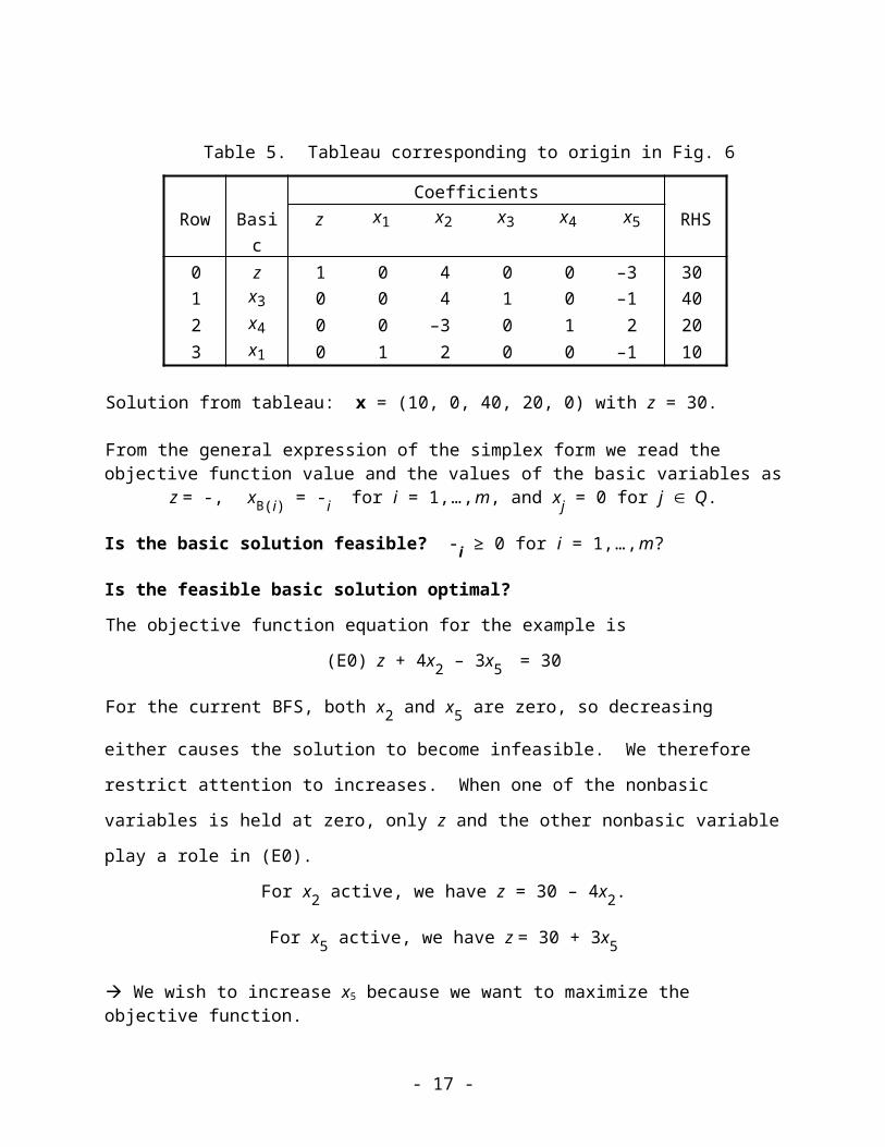
Table 8. Tableau with ratios computed
CoefficientsRow Basic RHS Ratio
0 1 -2 -3 0 0 0 0 ---1 0 -1 1 1 0 0 5 52 0 1 3 0 1 0 35 11.673 0 1 0 0 0 1 20 ---
x1zz
x2 x3 x4 x5
x3
x4
x5
Table 9. Tableau after iteration 1
CoefficientsRow Basic RHS Ratio
0 1 -5 0 3 0 0 15 ---1 0 -1 1 1 0 0 5 ---2 0 4 0 -3 1 0 20 53 0 1 0 0 0 1 20 20
x1zz
x2 x3 x4 x5
x4
x5
x2
To economize on tables, we show both the results of the current iteration and the selection of the entering and leaving variables for the next iteration in the same tableau. For example, Table 9 shows the results of iteration 1 and the selections for iteration 2.
Iteration 2
Step 2 (Iterate - update tableau)
a. Only x1 has a negative coefficient in row 0 so it is selected to enter the basis (s = 1).
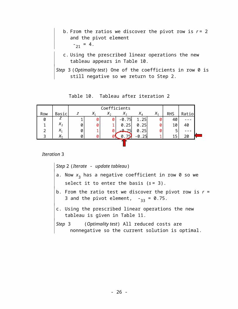
b. From the ratios we discover the pivot row is r = 2 and the pivot element -21 = 4.
c. Using the prescribed linear operations the new tableau appears in Table 10.
Step 3 (Optimality test) One of the coefficients in row 0 is still negative so we return to Step 2.
- 17 -
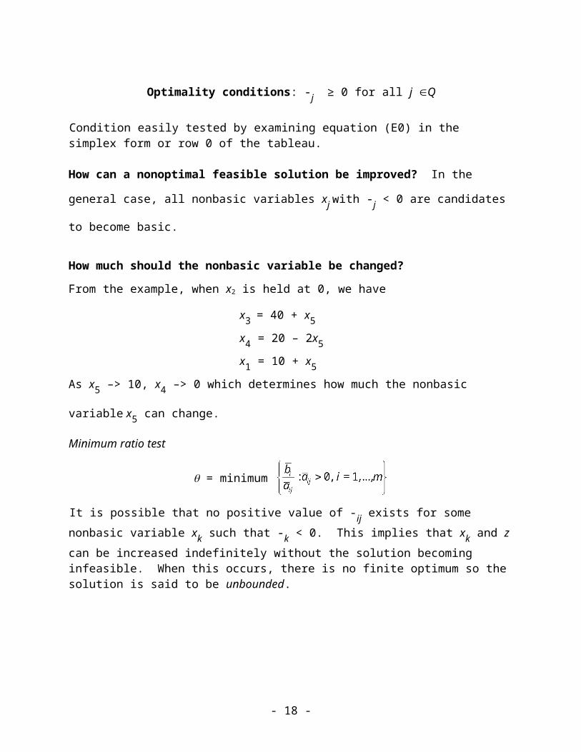
Table 10. Tableau after iteration 2
CoefficientsRow Basic RHS Ratio
0 1 0 0 -0.75 1.25 0 40 ---1 0 0 1 0.25 0.25 0 10 402 0 1 0 -0.75 0.25 0 5 ---3 0 0 0 0.75 -0.25 1 15 20
x1zz
x2 x3 x4 x5
x2
x1
x5
Iteration 3
Step 2 (Iterate - update tableau)
a. Now x3 has a negative coefficient in row 0 so we select it to enter the basis (s = 3).
b. From the ratio test we discover the pivot row is r = 3 and the pivot element, -33 = 0.75.
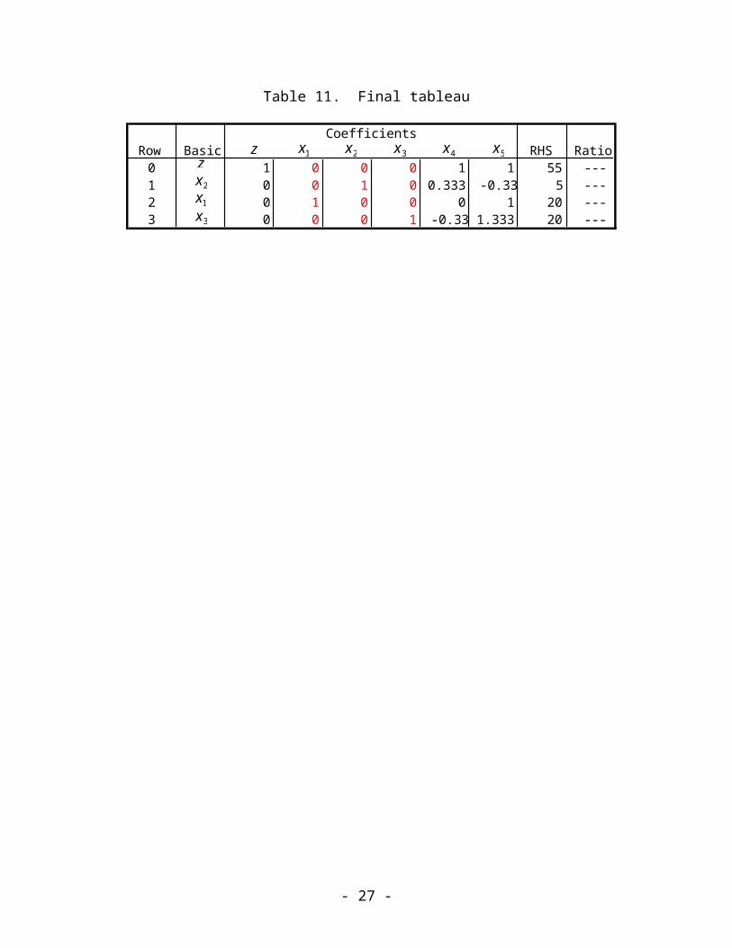
c. Using the prescribed linear operations the new tableau is given in Table 11.
Step 3 (Optimality test) All reduced costs are nonnegative so the current solution is optimal.
Table 11. Final tableau
CoefficientsRow Basic RHS Ratio
0 1 0 0 0 1 1 55 ---1 0 0 1 0 0.333 -0.33 5 ---2 0 1 0 0 0 1 20 ---3 0 0 0 1 -0.33 1.333 20 ---
x1zz
x2 x3 x4 x5
x2
x1
x3
- 18 -
3.7 Special Situations
Tie for the Entering Variable: Arbitrarily select one (the first).
Tie for the Leaving Variable: this will lead to a degenerate BFS.
Definition 8: A basic solution x n is said to be degenerate if the number of structural
constraints and nonnegativity conditions active at x is greater than n.
In two dimensions, a degenerate basic solution occurs at the intersection of three or more lines;
in three dimensions, a degenerate solution is at the intersection of four or more hyperplanes.
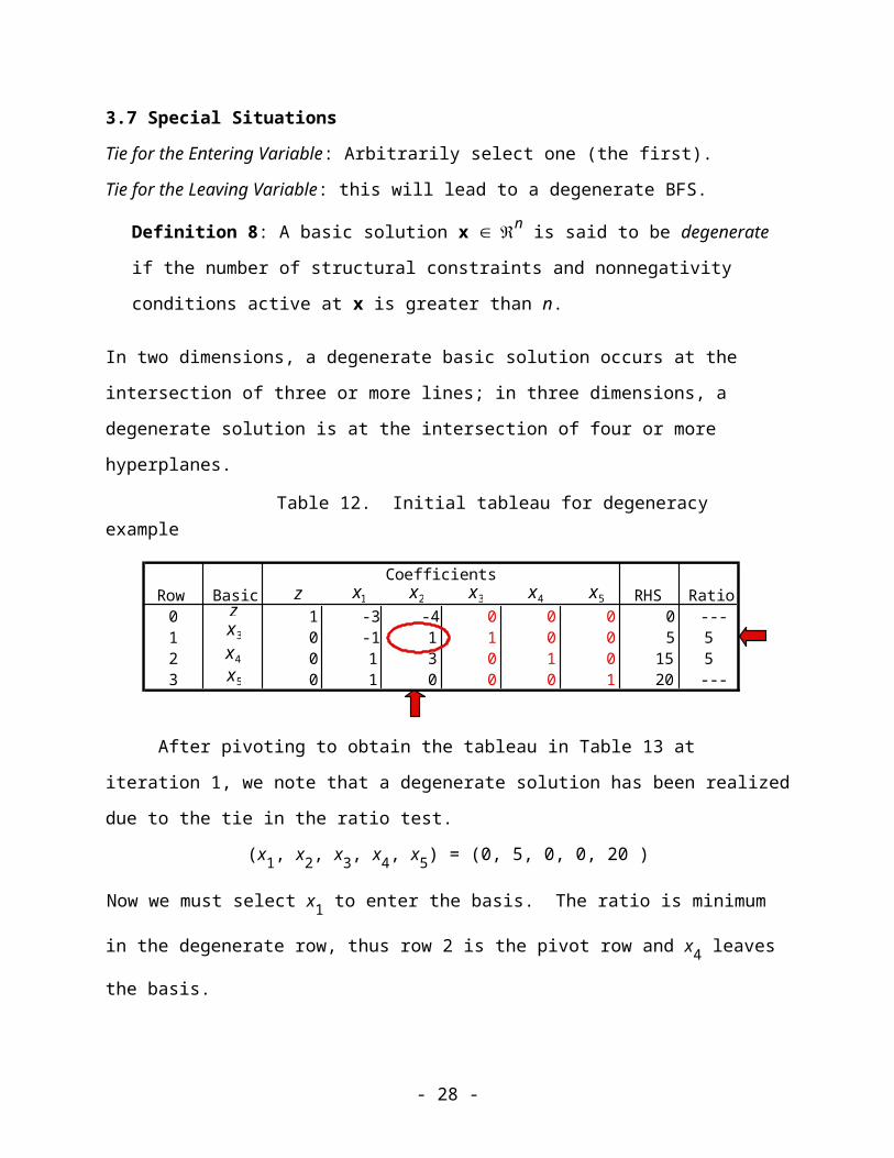
Table 12. Initial tableau for degeneracy example
CoefficientsRow Basic RHS Ratio
0 1 -3 -4 0 0 0 0 ---1 0 -1 1 1 0 0 5 52 0 1 3 0 1 0 15 53 0 1 0 0 0 1 20 ---
x1zz
x2 x3 x4 x5
x3
x4
x5
After pivoting to obtain the tableau in Table 13 at iteration 1, we note that a degenerate
solution has been realized due to the tie in the ratio test.
(x1, x2, x3, x4, x5) = (0, 5, 0, 0, 20 )
Now we must select x1 to enter the basis. The ratio is minimum in the degenerate row, thus row
2 is the pivot row and x4 leaves the basis.
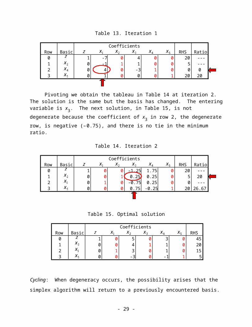
Table 13. Iteration 1
CoefficientsRow Basic RHS Ratio
0 1 -7 0 4 0 0 20 ---1 0 -1 1 1 0 0 5 ---2 0 4 0 -3 1 0 0 03 0 1 0 0 0 1 20 20
x1zz
x2 x3 x4 x5
x5
x2
x4
Pivoting we obtain the tableau in Table 14 at iteration 2. The solution is the same but the basis has changed. The entering variable is x3. The next solution, in Table 15, is not degenerate because the coefficient of x3 in row 2, the degenerate row, is negative (–0.75), and there is no tie in the minimum ratio.
- 19 -
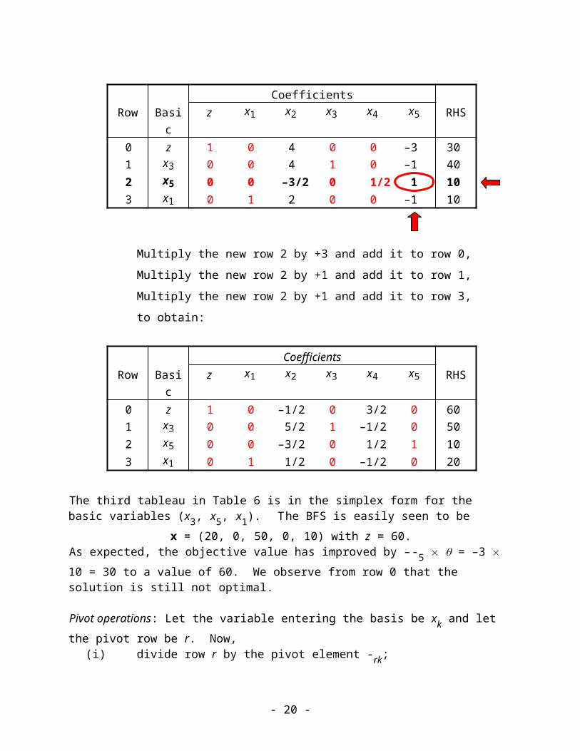
Table 14. Iteration 2
CoefficientsRow Basic RHS Ratio
0 1 0 0 -1.25 1.75 0 20 ---1 0 0 1 0.25 0.25 0 5 202 0 1 0 -0.75 0.25 0 0 ---3 0 0 0 0.75 -0.25 1 20 26.67
x1zz
x2 x3 x4 x5
x5
x2
x1
Table 15. Optimal solution
CoefficientsRow Basic RHS
0 1 0 5 0 3 0 451 0 0 4 1 1 0 202 0 1 3 0 1 0 153 0 0 -3 0 -1 1 5
x1zz
x2 x3 x4 x5
x5
x1
x3
Cycling: When degeneracy occurs, the possibility arises that the simplex algorithm will return to
a previously encountered basis. Nevertheless, cycling can be eliminated by modifying the rules
used to select the entering and leaving variables. The rules are based on the indices of the
problem variables, xj (j = 1,…,n) and are due to Bland (1977).
Rule for selecting the entering variable: From all the variables having negative coefficients in row 0, select the one with the smallest index to enter the basis.
Rule for selecting the leaving variable: Use the standard ratio test to select the leaving variable, but if there is a tie in the ratio test, select from the tied rows the variable having the smallest index.
Alternative optima: If the optimal tableau shows one or more nonbasic variables with zero
coefficients in row 0, there are alternative optimal solutions.
If x1,…,xs are optimal BFSs, then so is ^ where
^ = , = 1, k ≥ 0, k = 1,…,s
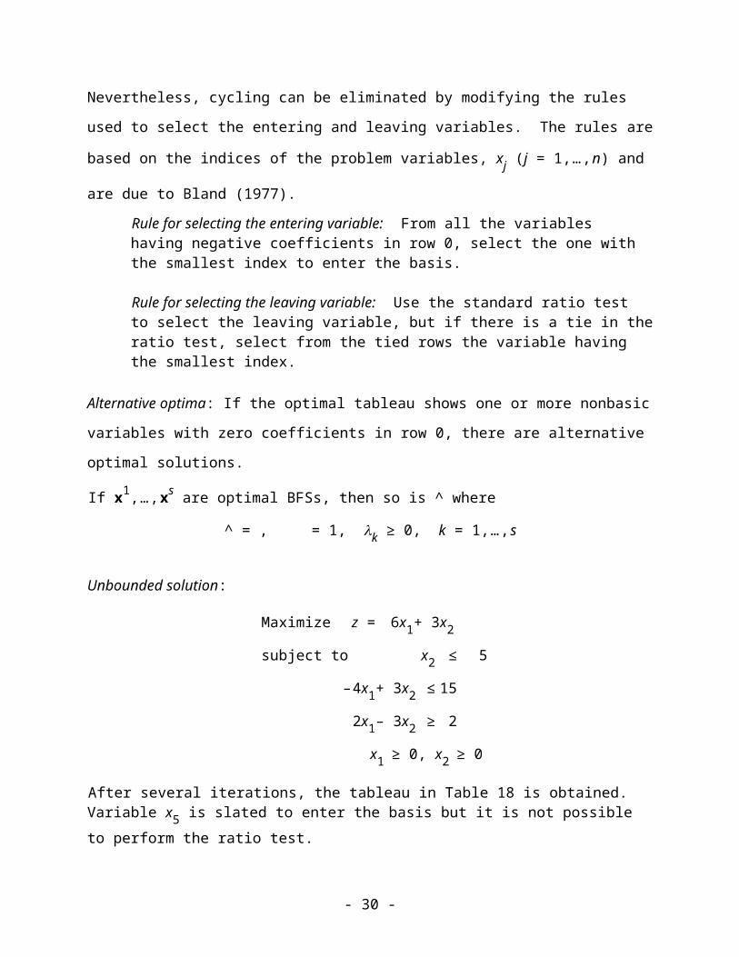
Unbounded solution:
- 20 -
Maximize z = 6x1 + 3x2
subject to x2 ≤ 5
–4x1 + 3x2 ≤ 15
2x1 – 3x2 ≥ 2
x1 ≥ 0, x2 ≥ 0
After several iterations, the tableau in Table 18 is obtained. Variable x5 is slated to enter the basis but it is not possible to perform the ratio test.
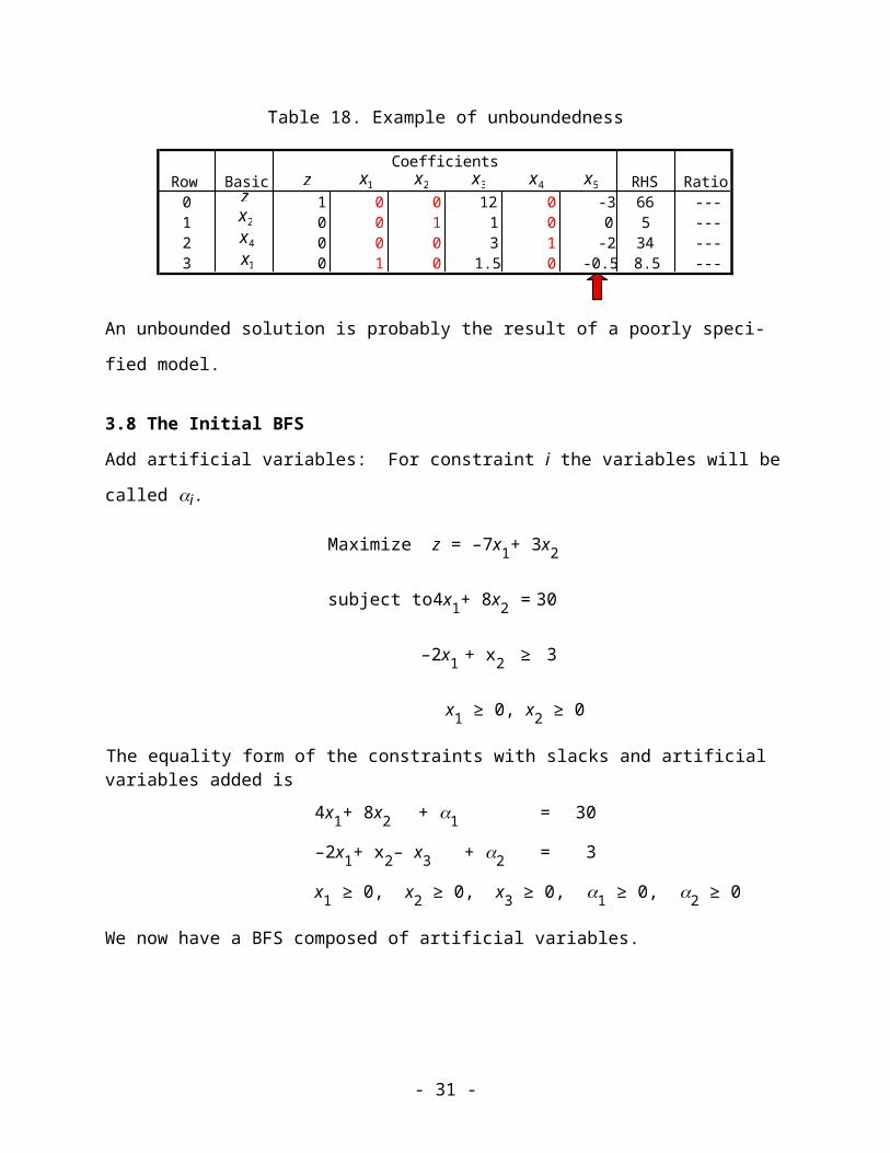
Table 18. Example of unboundedness
CoefficientsRow Basic RHS Ratio
0 1 0 0 12 0 -3 66 ---1 0 0 1 1 0 0 5 ---2 0 0 0 3 1 -2 34 ---3 0 1 0 1.5 0 -0.5 8.5 ---
x1zz
x2 x3 x4 x5
x4
x1
x2
An unbounded solution is probably the result of a poorly specified model.
3.8 The Initial BFS
Add artificial variables: For constraint i the variables will be called i.
Maximize z = –7x1+ 3x2
subject to 4x1 + 8x2 = 30
–2x1 + x2 ≥ 3
x1 ≥ 0, x2 ≥ 0
The equality form of the constraints with slacks and artificial variables added is
4x1+ 8x2 + 1 = 30
–2x1+ x2 – x3 + 2 = 3
x1 ≥ 0, x2 ≥ 0, x3 ≥ 0, 1 ≥ 0, 2 ≥ 0
We now have a BFS composed of artificial variables.
- 21 -
Algorithm for the Two-Phase Method
Initial step: Put the problem into equality form adding slack and artificial variables has necessary. Let F be the set of constraints that have artificial variables.
Phase 1: Solve
Minimize
where i is present in constraint i only if i F. If some artificial variables remain in the basis at
a zero level, the constraints for which they are basic are redundant and can be deleted.
Phase 2: Delete the artificial variables from the problem and revert to the original objective function
Maximize
Starting from the BFS obtained at the termination of phase 1, use the simplex method to solve
the original problem to optimality.
Example
Phase 1: Maximize w = – 1 – 2
Phase 2: Maximize z = –7x1 + 3x2
subject to 4x1 + 8x2 + 1 = 30
– 2x1 + x2 – x3 + 2 = 3
x1 ≥ 0, x2 ≥ 0, x3 ≥ 0, 1 ≥ 0, 2 ≥ 0
In constructing the tableau in Table 19, we introduce row 0' for the phase 1 objective.
Row 0' is not in the simplex form because the coefficients of the basic variables 1 and 2 are
not zero. To price out these coefficients we subtract row 1 and row 2 from row 0' with the result
shown in row 0 which is now used for the Phase 1 computations.
- 22 -
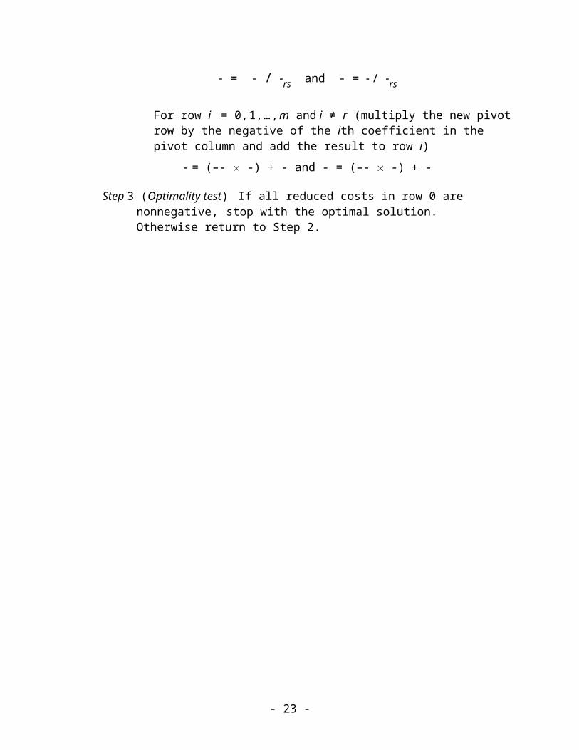
Table 19. Initial tableau for phase 1
CoefficientsRow Basic RHS Ratio
0' 1 0 0 0 1 1 00 1 -2 -9 1 0 0 -33 ---1 0 4 8 0 1 0 30 3.752 0 -2 1 -1 0 1 3 3
x1 x2 x3 1 2
2
1
ww
w
Table 20. Iteration 1
CoefficientsRow Basic RHS Ratio
0 1 -20 0 -8 0 9 -6 ---1 0 20 0 8 1 -8 6 0.32 0 -2 1 -1 0 1 3 ---
x1 x2 x3 1 2
1
x2
ww
Table 21. Optimal solution for phase 1
CoefficientsRow Basic RHS Ratio
0 1 0 0 0 1 1 0 ---1 0 1 0 0.4 0.05 -0.4 0.3 ---2 0 0 1 -0.2 0.1 0.2 3.6 ---
x1 x2 x3 1 2
x2
x1
ww
Phase 2 is initiated with the basic solution (x1, x2, x3) = (0.3, 3.6, 0) found in phase 1. As shown in Table 22, we put the phase 2 objective function in row 0'. Again we find that the tableau is not in the simplex form so we price out the nonzero coefficients in the columns for the basic variables. The result is labeled row 0.
- 23 -
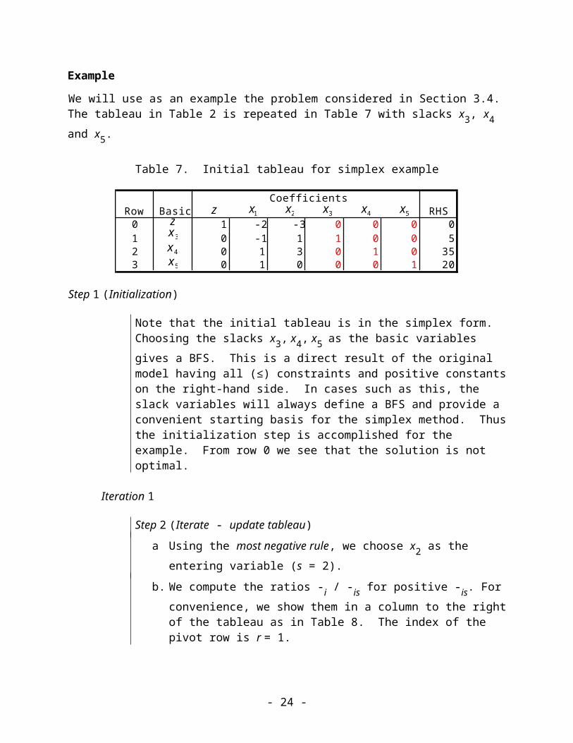
Table 22. Initial solution for phase 2
CoefficientsRow Basic z x1 x2 x3 RHS Ratio
0' z 1 7 –3 0 00 z 1 0 0 –3.4 8.7 --1 x1 0 1 0 0.4 0.3 0.752 x2 0 0 1 –0.2 3.6 --
Table 23. Optimum solution for phase 2
CoefficientsRow Basic RHS Ratio
0 1 8.5 0 0 11.25 ---1 0 2.5 0 1 0.75 ---2 0 0.5 1 0 3.75 ---
x1zz
x2 x3
x2
x3
3.9 Dual Simplex Algorithm
The dual simplex algorithm is most suited for problems where an initial dual feasible solution
available. It is particularly useful for reoptimizing a problem after a constraint has been added or
some parameters have been changed so that the previously optimal basis is no longer feasible.
Step 1 (Initialization)
Start with a dual feasible basis and let k = 1. Create a tableau for this basis in the simplex form. If the right-hand side entries are all nonnegative, the solution is primal feasible, so stop with the optimal solution.
Step 2 (Iteration k)
a. Select the leaving variable. Find a row, call it r, with a negative right-hand-side constant; i.e., -r < 0. Let row r be the pivot row and let the leaving variable be xB(r). A common rule for choosing r is to select the most negative RHS value; i.e.,
-r = min{-i : i = 1,…,m}.
- 24 -
b. Determine the entering variable. For each negative coefficient in the pivot row, compute the negative of the ratio between the reduced cost in row 0 and the structural coefficient in row r. If there is no negative coefficient, -rj < 0, stop; there is no feasible solution.
Let the column with the minimum ratio, designated by the index s, be the pivot column; let xs is the entering variable. The pivot column is determined by the following ratio test.
= min
c. Change the basis. Replace xB(r) by xs in the basis. Create a new tableau by performing the following operations (these are the same as for the primal simplex algorithm).
Let - be the vector of the ith row of the current tableau, and let - be the ith row in the new tableau. Let - be the RHS for row i in the current tableau, and let - be the RHS of the new tableau. Let - be the element in the ith row of the pivot column s.
The pivot row in the new tableau is
- = - / - and - = - /-.
The other rows in the new tableau are
- = + - and
- = + - for i = 0,1,…,m, i ≠ r
(These operations have the effect of pricing out the pivot column. Its replacement will have a single 1 in row r and a zero in all other rows as required by the simplex form.)
Step 3 (Feasibility test)
If all entries on the right-hand side are nonnegative the solution is primal feasible, so stop with the optimal solution. Otherwise, put k k +1 and return to Step 2.
3.10 Simplex Method Using Matrix Notation
Decision variables: x = (x1,…,xn)T
- 25 -
Objective coefficients: c = (c1,…,cn)
Right-hand-side constants: b = (b1,…,bm)T
Structural coefficients: A =
Making use of this notation, Eqs. (1) – (3) can be rewritten as
Maximize z = cx
subject to Ax = b
x ≥ 0
Example
Maximize z = 2x1 + 1.25x2 + 3x3
subject to 2x1 + x2 + 2x3 ≤ 7
3x1 + x2 ≤ 6
x2 + 6x3 ≤ 9
x1 ≥ 0, x2 ≥ 0, x3 ≥ 0
With x4, x5 and x6 as slacks, the matrices and vectors defining the equality form of the model are:
x = (x1, x2, x3, x4, x5, x6)T
c = (2, 1.25, 3, 0, 0, 0)
A = and b =
Computing a Basic Solution
Let x = (xB, xN), where xB and xN refer to the basic and nonbasic variables, respectively. Let A = (B, N), where B is the m m basis matrix and N is m (n – m). The equations Ax = b can thus be written
(B, N) = BxB + NxN = b.
Multiplying through be B–1 gives
xB + B–1NxN = B–1b.
Solving this set of equations allows us to express the basic variables in terms of the nonbasic variables.
- 26 -
xB = B–1(b – NxN).
The objective function can be written as the sum of two terms, one for the basic variables and the other for the nonbasic variables:
z = cBxB + cNxN = cBB–1(b – NxN) + cNxN (7)
A basic solution is found by setting the nonbasic variables to zero, xN = 0, so
xB = B–1b and z = cBB–1b
For convenience and later use in the section on the revised simplex method, we introduce the m-dimensional row vector of dual variables, π, and define it as
π cBB–1
so z = πb.
For the example, when xB = (x1,x3,x5)T, the basic solution is
xB = B–1b = =
with objective value
z = cBxB = (2, 3, 0) = 8.5
and dual solution
π = (π1, π2, π3) = cBB–1
= (2, 3, 0) = (1, 0, 1/6).
Marginal Information Concerning the Objective
From Eq. (7) we see that the objective function value for a given basis can be written as
z = cBB–1b + (cN – cBB–1N)xN
For consistency with the material in the sections on the simplex tableau, we will work with the
above equation in the following form:
z = cBB–1b – (cBB–1N – cN)xN
We want to hold all the nonbasic variables to zero except one, xk, and observe the effect.
The column for xk in N is the same as the column for xk in A; call it Ak. The objective value as a
function of xk alone is
- 27 -
z = cBB–1b – (cBB–1Ak – ck)xk.
The first term on the right of this expression is a constant for a given basis. The coefficient of xk
in the second term (without the “–” sign) is the marginal change in the objective function for a
unit increase in xk. Define for the general nonbasic variable xk, the marginal change
-k = cBB–1Ak – ck = πAk – ck (8)
where -k is what we called the reduced cost of xk.
A sufficient condition for a given basis to be optimal is that increasing any nonbasic
variable will cause the object to decrease or stay the same.
-k ≥ 0 for all k Q
If this condition is not satisfied, every nonbasic variable with a negative marginal value is a
candidate to enter the basis.
For the example, the nonbasic variables are xN = (x2, x4, x6) with cN =(1.25, 0, 0) and π = (1, 0, 1/6). The reduced cost for each of the nonbasic variables is computed using Eq. (8) as follows:
for x2 we have -2 = (1, 0, 1/6) (1, 1, 1)T – 1.25 = –1/12,
for x4 we have -4 = (1, 0, 1/6) (1, 0, 0)T – 0 = 1,
for x6 we have -6 = (1,0,1/6) (0, 0, 1)T – 0 = 1/6.
Matrix Representation of the Simplex Tableau
Given a basis and basis inverse, the matrix representation of an LP can be written as
= (9)
which is equivalent to equations (E0), (Ei), i = 1,…,m, in Section 3.4. The RHS of (9) is .
3.11 Revised Simplex Method
Not necessary to keep track of the entire tableau, on current basis inverse. Following
information required
• Primal variables: xB = B–1b
- 28 -
• Dual variables: π = cBB–1
• Marginal cost for xk: -k = πAk – ck (Ak is the kth column of A)
• Pivot column: -k = B–1Ak
Statement of the Algorithm
Algorithm presented in parallel with the example introduced in Section 3.10. The starting tableau is given in Table 3.35.
Table 35. Tableau for example
CoefficientsRow Basic RHS
0 1 0 -0.083 0 1 0 0.1667 8.51 0 1 0.3333 0 0.5 0 -0.167 22 0 0 0.1667 1 0 0 0.1667 1.53 0 0 0 0 -1.5 1 0.5 0
x1z x2
zx1
x3 x4 x5 x6
x3
x5
Let,
xB = (x1, x3, x5)T, cB = (2, 3, 0),
B = and B–1 = .
Step 1. Compute the basic solution.
For the current basis B, compute B–1 and the primal and dual solutions
xB = B–1b, π = cBB–1.
For the example, using B–1 above, we compute
xB = (x1, x3, x5)T = (2, 3/2, 0)T
π = (π1, π2, π3) = (1, 0, 1/6).
Step 2. Select the variable to enter the basis .
For each nonbasic variable, compute the reduced cost
-j = πAj – cj
If each of these values in nonnegative, stop with the optimal solution and compute z* =
As we have seen, for x2,
-2 = (1, 0, 1/6) (1, 1, 1)T – 1.25 = –1/12,
for x4, -4 = (1, 0, 1/6) (1,0,0)T – 0 = 1, and
for x6, -6 = (1,0,1/6) (0, 0, 1)T – 0 = 1/6.
Since the reduced cost for x2 is negative,
- 29 -
cBxB. Otherwise, select the variable with
most negative reduced cost to enter the basis. The entering variable is xs.
the solution can be improved by allowing x2 to enter the basis (s = 2).
Step 3. Compute the pivot column.
Let column s of the matrix A be the vector As. Compute the pivot column
-s = B–1As.
For s = 2, the pivot column is
-2 = B–1(1, 1, 1)T = (1/3, 1/6, 0)T.
Step 4. Find the variable to leave the basis.
Find the row r for which the minimum ratio is obtained; i.e.,
= xB(r) / -rs
= min
If there are no rows that have -is > 0, the
solution is unbounded. Otherwise, the basic variable xB(r) leaves the basis; is the amount that the variable xs is to increase in order drive xB(r) to zero.
At the current iteration,
= min = 6,
with the minimum obtained for row 1.Thus x1 will leave the basis as x2 increases from 0 to 6. Note that x1 is the basic
variable for row 1. It is important to keep tract of this correspondence.
Step 5. Change the basis.
Replace xB(r) by xs in set of basic variables and replace cB(r) by cs in cB. Update the
basis inverse (this is equivalent to pivoting in the simplex tableau). Return to Step 1.
For the new basis
xB = (x2, x3, x5)T, cB = (1.25, 3, 0)
The new basis inverse is
B–1 = .
We now go to Step 1.
- 30 -
The algorithm continues until the optimality condition is met at Step 2 or an unbounded
solution is discovered at Step 4. For the example problem, the new BFS is solution is discovered
at Step 4. For the example problem, the new BFS is
xB = (x2, x3, x5)T = (6, 1/2, 0)T with z = cBxB = 9.
which is an improvement over the initial basic BFS whose objective function value is z = 8.5, as
seen in Table 35.
Table 35. Tableau for example
CoefficientsRow Basic RHS
0 1 0 -0.083 0 1 0 0.1667 8.51 0 1 0.3333 0 0.5 0 -0.167 22 0 0 0.1667 1 0 0 0.1667 1.53 0 0 0 0 -1.5 1 0.5 0
x1z x2
zx1
x3 x4 x5 x6
x3
x5
- 31 -


![[Nayfeh a.H., Chin C.-m.] Perturbation Methods](https://img.pdfslide.us/doc/110x75/577cd1261a28ab9e7893bd4c/nayfeh-ah-chin-c-m-perturbation-methods.jpg)