Chapter 3 Learn by Doing: Analyze a Light Pipe

LightTools Introductory Tutorial • 25

Chapter 3 Learn by Doing: Analyze a Light Pipe

In this chapter, you open, view, ray trace, and modify a simple plastic light pipe. Then, you do some basic illumination analysis, introduce a scattering surface, and see the effect of this on the illumination distribution. This introduces you to many of the basic techniques needed to use LightTools.

Contents

What is a Light Pipe? ..............................................................................................26

Opening, Viewing, and Selecting............................................................................27

Tracing Rays and Modifying the Light Pipe...........................................................32

Performing Illumination Analysis...........................................................................40

Optical Properties Example: Paint It White ............................................................49

Conclusions.............................................................................................................51

26 • LightTools Introductory Tutorial

CHAPTER 3 Learn by Doing: Analyze a Light Pipe

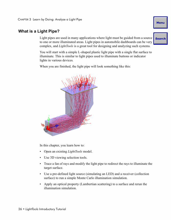
What is a Light Pipe?Light pipes are used in many applications where light must be guided from a source to one or more illuminated areas. Light pipes in automobile dashboards can be very complex, and LightTools is a great tool for designing and analyzing such systems.

You will start with a simple L-shaped plastic light pipe with a single flat surface to illuminate. This is similar to light pipes used to illuminate buttons or indicator lights in various devices.

When you are finished, the light pipe will look something like this:

In this chapter, you learn how to:

• Open an existing LightTools model.

• Use 3D viewing selection tools.

• Trace a fan of rays and modify the light pipe to redirect the rays to illuminate the target surface.

• Use a pre-defined light source (simulating an LED) and a receiver (collection surface) to run a simple Monte Carlo illumination simulation.

• Apply an optical property (Lambertian scattering) to a surface and rerun the illumination simulation.



This will allow you to exercise many powerful LightTools features in a short time. Some of these features are briefly explained as they are introduced here, and additional explanation is included in subsequent chapters. The main purpose of this chapter is to get familiar with the interface and with typical tasks and procedures.

This is a very simple system, but it allows you to explore some of LightTools basic features.

Opening, Viewing, and SelectingThe starting point for this light pipe model is supplied with the sample models in the LightTools installation directory. It is made of plastic (polycarbonate) and consists of two blocks joined using Boolean operations, with a simple light source, and a rectangular dummy element (that is, an element that has no optical effect) with a receiver for illumination analysis. The source and receiver are on a hidden layer, so you won't see them at first.

Opening the Model

1. Select File > Open on the menu bar.

If you didn’t close your model after you finished setting preferences, a LightTools message is displayed warning that your model hasn’t been saved. Click OK to close it now and continue.

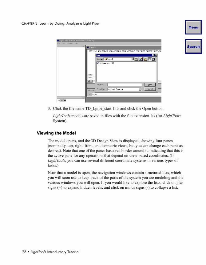
2. On the Open dialog box, browse to the \Tutorial folder of the LightTools installation directory, shown in the following figure.

Note: Be sure that you have set your preferences as described in Chapter 2.



3. Click the file name TD_Lpipe_start.1.lts and click the Open button.

LightTools models are saved in files with the file extension .lts (for LightTools System).

Viewing the ModelThe model opens, and the 3D Design View is displayed, showing four panes (nominally, top, right, front, and isometric views, but you can change each pane as desired). Note that one of the panes has a red border around it, indicating that this is the active pane for any operations that depend on view-based coordinates. (In LightTools, you can use several different coordinate systems in various types of tasks.)

Now that a model is open, the navigation windows contain structured lists, which you will soon use to keep track of the parts of the system you are modeling and the various windows you will open. If you would like to explore the lists, click on plus signs (+) to expand hidden levels, and click on minus signs (-) to collapse a list.



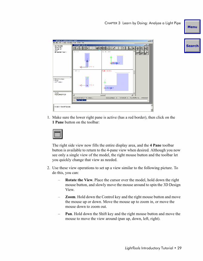
1. Make sure the lower right pane is active (has a red border), then click on the 1 Pane button on the toolbar:

The right side view now fills the entire display area, and the 4 Pane toolbar button is available to return to the 4-pane view when desired. Although you now see only a single view of the model, the right mouse button and the toolbar let you quickly change that view as needed.

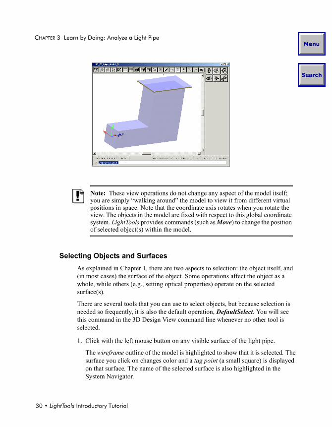
2. Use these view operations to set up a view similar to the following picture. To do this, you can:

– Rotate the View. Place the cursor over the model, hold down the right mouse button, and slowly move the mouse around to spin the 3D Design View.

– Zoom. Hold down the Control key and the right mouse button and move the mouse up or down. Move the mouse up to zoom in, or move the mouse down to zoom out.

– Pan. Hold down the Shift key and the right mouse button and move the mouse to move the view around (pan up, down, left, right).



Selecting Objects and SurfacesAs explained in Chapter 1, there are two aspects to selection: the object itself, and (in most cases) the surface of the object. Some operations affect the object as a whole, while others (e.g., setting optical properties) operate on the selected surface(s).

There are several tools that you can use to select objects, but because selection is needed so frequently, it is also the default operation, DefaultSelect. You will see this command in the 3D Design View command line whenever no other tool is selected.

1. Click with the left mouse button on any visible surface of the light pipe.

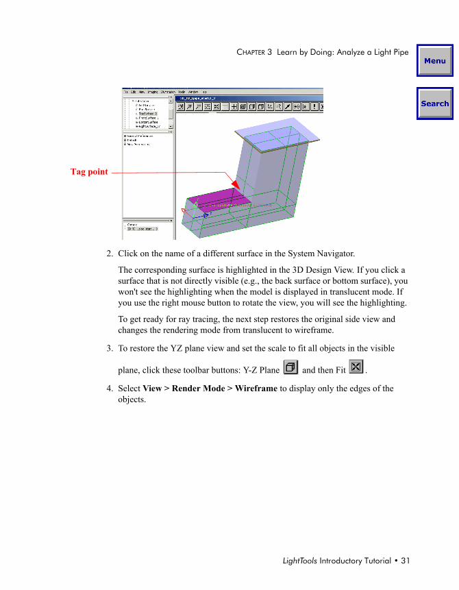
The wireframe outline of the model is highlighted to show that it is selected. The surface you click on changes color and a tag point (a small square) is displayed on that surface. The name of the selected surface is also highlighted in the System Navigator.

Note: These view operations do not change any aspect of the model itself; you are simply “walking around” the model to view it from different virtual positions in space. Note that the coordinate axis rotates when you rotate the view. The objects in the model are fixed with respect to this global coordinate system. LightTools provides commands (such as Move) to change the position of selected object(s) within the model.



2. Click on the name of a different surface in the System Navigator.

The corresponding surface is highlighted in the 3D Design View. If you click a surface that is not directly visible (e.g., the back surface or bottom surface), you won't see the highlighting when the model is displayed in translucent mode. If you use the right mouse button to rotate the view, you will see the highlighting.

To get ready for ray tracing, the next step restores the original side view and changes the rendering mode from translucent to wireframe.

3. To restore the YZ plane view and set the scale to fit all objects in the visible

plane, click these toolbar buttons: Y-Z Plane and then Fit .

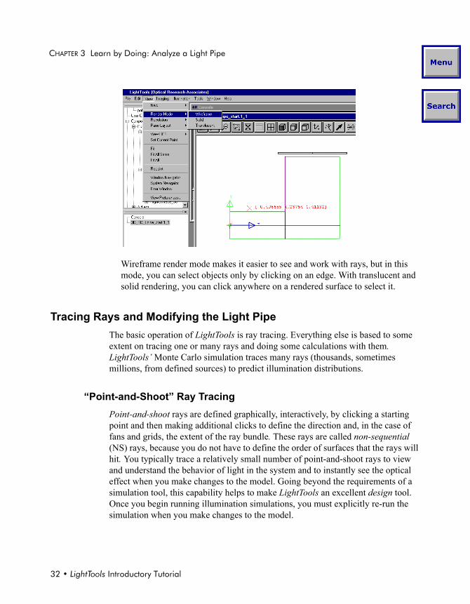
4. Select View > Render Mode > Wireframe to display only the edges of the objects.

Tag point



Wireframe render mode makes it easier to see and work with rays, but in this mode, you can select objects only by clicking on an edge. With translucent and solid rendering, you can click anywhere on a rendered surface to select it.

Tracing Rays and Modifying the Light PipeThe basic operation of LightTools is ray tracing. Everything else is based to some extent on tracing one or many rays and doing some calculations with them. LightTools’ Monte Carlo simulation traces many rays (thousands, sometimes millions, from defined sources) to predict illumination distributions.

“Point-and-Shoot” Ray TracingPoint-and-shoot rays are defined graphically, interactively, by clicking a starting point and then making additional clicks to define the direction and, in the case of fans and grids, the extent of the ray bundle. These rays are called non-sequential (NS) rays, because you do not have to define the order of surfaces that the rays will hit. You typically trace a relatively small number of point-and-shoot rays to view and understand the behavior of light in the system and to instantly see the optical effect when you make changes to the model. Going beyond the requirements of a simulation tool, this capability helps to make LightTools an excellent design tool. Once you begin running illumination simulations, you must explicitly re-run the simulation when you make changes to the model.



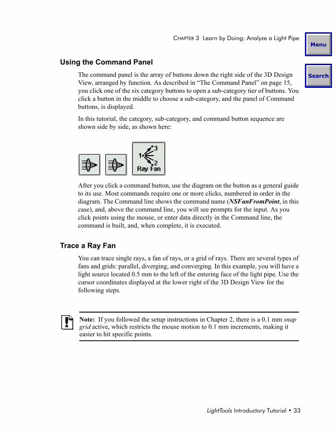
Using the Command PanelThe command panel is the array of buttons down the right side of the 3D Design View, arranged by function. As described in “The Command Panel” on page 15, you click one of the six category buttons to open a sub-category tier of buttons. You click a button in the middle to choose a sub-category, and the panel of Command buttons, is displayed.

In this tutorial, the category, sub-category, and command button sequence are shown side by side, as shown here:

After you click a command button, use the diagram on the button as a general guide to its use. Most commands require one or more clicks, numbered in order in the diagram. The Command line shows the command name (NSFanFromPoint, in this case), and, above the command line, you will see prompts for the input. As you click points using the mouse, or enter data directly in the Command line, the command is built, and, when complete, it is executed.

Trace a Ray FanYou can trace single rays, a fan of rays, or a grid of rays. There are several types of fans and grids: parallel, diverging, and converging. In this example, you will have a light source located 0.5 mm to the left of the entering face of the light pipe. Use the cursor coordinates displayed at the lower right of the 3D Design View for the following steps.

Note: If you followed the setup instructions in Chapter 2, there is a 0.1 mm snap grid active, which restricts the mouse motion to 0.1 mm increments, making it easier to hit specific points.



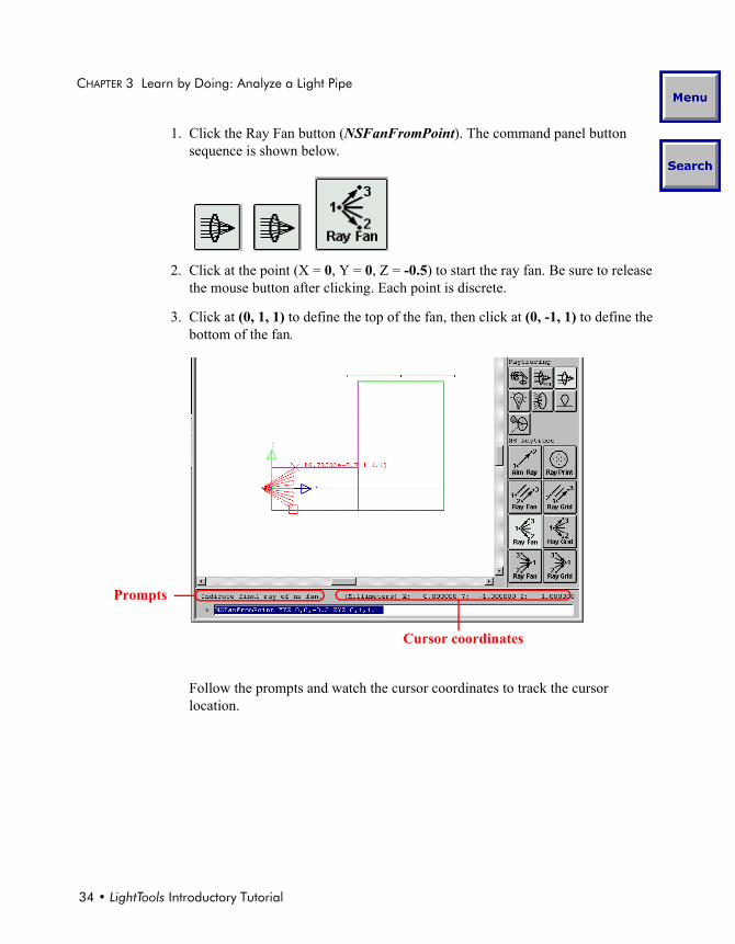
1. Click the Ray Fan button (NSFanFromPoint). The command panel button sequence is shown below.

2. Click at the point (X = 0, Y = 0, Z = -0.5) to start the ray fan. Be sure to release the mouse button after clicking. Each point is discrete.

3. Click at (0, 1, 1) to define the top of the fan, then click at (0, -1, 1) to define the bottom of the fan.

Follow the prompts and watch the cursor coordinates to track the cursor location.

Prompts

Cursor coordinates



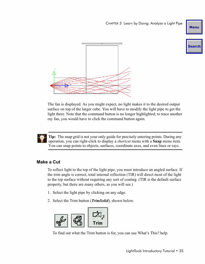
The fan is displayed. As you might expect, no light makes it to the desired output surface on top of the larger cube. You will have to modify the light pipe to get the light there. Note that the command button is no longer highlighted; to trace another ray fan, you would have to click the command button again.

Make a CutTo reflect light to the top of the light pipe, you must introduce an angled surface. If the trim angle is correct, total internal reflection (TIR) will direct most of the light to the top surface without requiring any sort of coating. (TIR is the default surface property, but there are many others, as you will see.)

1. Select the light pipe by clicking on any edge.

2. Select the Trim button (TrimSolid), shown below.

To find out what the Trim button is for, you can use What’s This? help.

Tip: The snap grid is not your only guide for precisely entering points. During any operation, you can right-click to display a shortcut menu with a Snap menu item. You can snap points to objects, surfaces, coordinate axes, and even lines or rays.



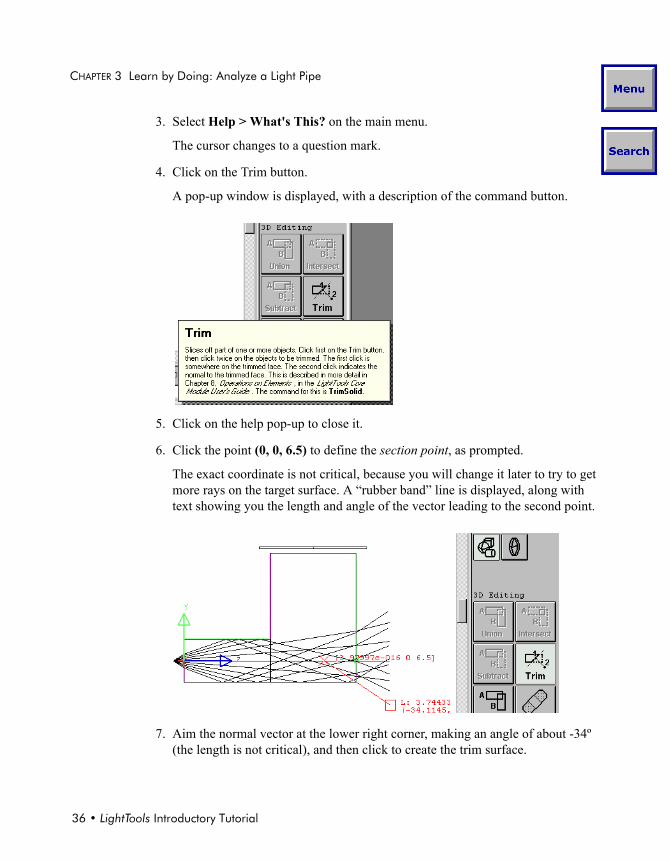
3. Select Help > What's This? on the main menu.

The cursor changes to a question mark.

4. Click on the Trim button.

A pop-up window is displayed, with a description of the command button.

5. Click on the help pop-up to close it.

6. Click the point (0, 0, 6.5) to define the section point, as prompted.

The exact coordinate is not critical, because you will change it later to try to get more rays on the target surface. A “rubber band” line is displayed, along with text showing you the length and angle of the vector leading to the second point.

7. Aim the normal vector at the lower right corner, making an angle of about -34º (the length is not critical), and then click to create the trim surface.



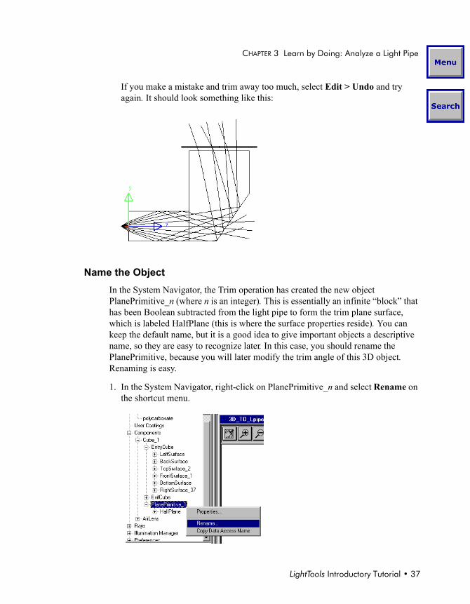
If you make a mistake and trim away too much, select Edit > Undo and try again. It should look something like this:

Name the ObjectIn the System Navigator, the Trim operation has created the new object PlanePrimitive_n (where n is an integer). This is essentially an infinite “block” that has been Boolean subtracted from the light pipe to form the trim plane surface, which is labeled HalfPlane (this is where the surface properties reside). You can keep the default name, but it is a good idea to give important objects a descriptive name, so they are easy to recognize later. In this case, you should rename the PlanePrimitive, because you will later modify the trim angle of this 3D object. Renaming is easy.

1. In the System Navigator, right-click on PlanePrimitive_n and select Rename on the shortcut menu.



2. Type a new name, such as TIR_fold, and press Enter.

3. Save the modified system:

a. Select File > Save As... .

b. Navigate to the \LTUser (or other) directory.

c. Key in a new name, such as Tut_Lpipe_trimmed.1.lts, and click Save.

Note that the file name displays in the title bar (top edge) of the 3D Design View window.

Changing PropertiesNow the light is getting to the collection surface, but it doesn't fill the surface and it isn’t very uniform. This is just a rough judgment based on a small number of rays, but it's often part of the iterative design process to use a few rays to make decisions about parameters, then do a Monte Carlo simulation to predict the illumination more precisely. It may not be possible to get a great distribution with a simple TIR surface, but it's easy to experiment with the angle and position of the trim surface.

1. In the System Navigator, right-click on TIR_fold (the recently renamed PlanePrimitive_n) and select Properties on the shortcut menu.

The Properties dialog box gives you access to every detail of a model, and it changes, depending on the type of object selected. Right now, it displays the Coordinates tab, which applies to the entire selected object. (There is also a navigation tree in the dialog box, which provides access to specific surfaces, but you don’t need to use it at this time.)



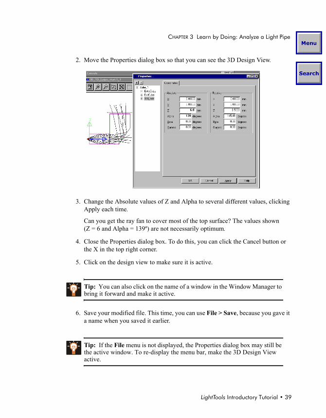
2. Move the Properties dialog box so that you can see the 3D Design View.

3. Change the Absolute values of Z and Alpha to several different values, clicking Apply each time.

Can you get the ray fan to cover most of the top surface? The values shown (Z = 6 and Alpha = 139º) are not necessarily optimum.

4. Close the Properties dialog box. To do this, you can click the Cancel button or the X in the top right corner.

5. Click on the design view to make sure it is active.

6. Save your modified file. This time, you can use File > Save, because you gave it a name when you saved it earlier.

Tip: You can also click on the name of a window in the Window Manager to bring it forward and make it active.

Tip: If the File menu is not displayed, the Properties dialog box may still be the active window. To re-display the menu bar, make the 3D Design View active.



Performing Illumination AnalysisPoint-and-shoot ray fans are great for simple analysis and design, because they instantly show you what the light does, but eventually you will want to simulate the illumination performance, which requires several additions to the model:

• One or more sources

• One or more receivers

• A few decisions, such as how many rays to trace, and whether or not to display them

• Various charting features, which enable you to look at analysis results

The light pipe model already has a source and receiver, but they are on a hidden layer. Next, you will display them and do some quick illumination simulations. Later examples will explain the illumination results more extensively.

LayersLightTools models can become very complex, with optical elements, mechanical parts, rays, sources, receivers, etc. The layer feature provides a way of managing this complexity, allowing you to separate objects on as many as 32 layers, any of which can be visible or hidden. A layer number is one of the properties assigned to a LightTools object. To see or set the layer number, right-click the object’s name in the System Navigation window, select the Properties shortcut menu and click on the Display tab.

In this model, a light source and receiver for illumination analysis have already been defined and hidden on layer 2. Follow these steps to make them visible.

1. Click on the design view.

2. Select Edit > Preferences to display the Preferences dialog box.

This dialog box controls many program parameters, with sections for General preferences, various defaults, and view-specific parameters for any views that are currently open (only the 3D Design view, in this case).

Note: Making a layer visible or hidden affects only the display of objects, not their optical behavior. For example, a mirror on a hidden layer still reflects rays. To make 3D objects “invisible” to rays, you must use another option: the Ray Traceable check box on the Ray Trace tab of the Properties dialog box.



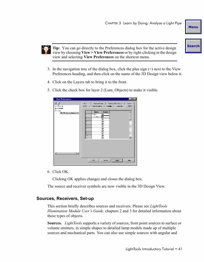
3. In the navigation tree of the dialog box, click the plus sign (+) next to the View Preferences heading, and then click on the name of the 3D Design view below it.

4. Click on the Layers tab to bring it to the front.

5. Click the check box for layer 2 (Lum_Objects) to make it visible.

6. Click OK.

Clicking OK applies changes and closes the dialog box.

The source and receiver symbols are now visible in the 3D Design View.

Sources, Receivers, Set-upThis section briefly describes sources and receivers. Please see LightTools Illumination Module User’s Guide, chapters 2 and 3 for detailed information about these types of objects.

Sources. LightTools supports a variety of sources, from point sources to surface or volume emitters, in simple shapes to detailed lamp models made up of multiple sources and mechanical parts. You can also use simple sources with angular and

Tip: You can go directly to the Preferences dialog box for the active design view by choosing View > View Preferences or by right-clicking in the design view and selecting View Preferences on the shortcut menu.



spatial distributions (apodization files) applied to match measured or desired distributions, as well as ray data sources created from measurements of real sources.

Receivers. Receivers are special objects created to collect ray trace data for illumination calculations. LightTools supports spatial and angular receivers, and they are usually attached to a surface of an object. (A far-field angular receiver is not attached to any object.) Receivers assign ray energy (weighted ray data) to bins (cells) in a collection mesh, and this allows the irradiance and other properties to be determined. There is a trade-off between radiometric accuracy (based on the number of rays per bin) and spatial accuracy (based on the number of bins across the receiver). LightTools allows you to re-bin the data without re-tracing the rays.

In this sample model, a source and surface receiver are already defined. The source is a 1.0 watt point source with an apodization file attached to simulate the Gaussian intensity of an LED. The receiver is attached to the rectangular dummy element (named AirLens in this model, because that's its material) defined for this purpose. You can attach receivers to surfaces of real objects or to dummy elements, depending on your goals.

Setup. Setup is a step that initializes various parameters to prepare for illumination analysis (using Illumination > Setup Simulation on the main menu). This step has already been done for this model, so you are ready to run a simulation.

Simulation Info and Ray PreviewA Monte Carlo simulation requires a large number of samples for accurate statistical estimates of illumination. Samples in LightTools are traced rays, but unlike point-and-shoot rays, rays in an illumination simulation are traced in random directions from randomly selected points in or on the defined sources. Apodization and other factors affect the selection of random points so source behavior can be accurately simulated.

Before tracing large numbers of Monte Carlo rays, it’s a good idea to trace a smaller number with the Ray Preview option turned on. When Ray Preview is on, LightTools draws the rays in the design view, allowing you to see whether or not things are working correctly. Drawing many rays may slow down the ray trace, so it makes sense to turn it off when you’re tracing thousands of rays (or more).

1. Select Illumination > Simulation Info to display the Illumination Simulation Properties dialog box.

2. Change the Total Rays to Trace to 200.



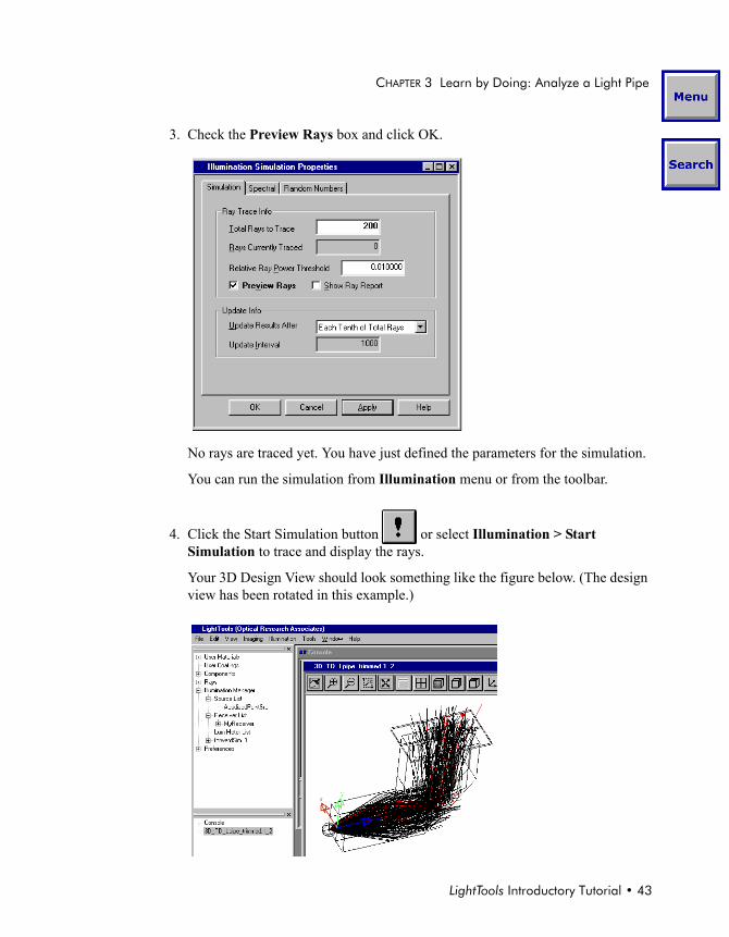
3. Check the Preview Rays box and click OK.

No rays are traced yet. You have just defined the parameters for the simulation.

You can run the simulation from Illumination menu or from the toolbar.

4. Click the Start Simulation button or select Illumination > Start Simulation to trace and display the rays.

Your 3D Design View should look something like the figure below. (The design view has been rotated in this example.)



Understanding ChartsWhen you run a simulation, all of the output data is stored in memory; you see the results when you open an illumination chart. Because there are many ways to view and analyze illumination results, the best chart to display depends on your goals. In this example, you will look only at the illuminance (spatial) distribution on the predefined surface receiver. Other available analyses and charts (including the interactive LumViewer) will be discussed in later examples.

Scatter charts are always a good starting point, because they are the closest thing to a view of the raw ray data. They don't tell you anything about the energy or statistics, but they allow you to see how completely you have covered the receiver.

1. With the 3D Design View active, select Illumination > Illuminance Display > Scatter Chart.

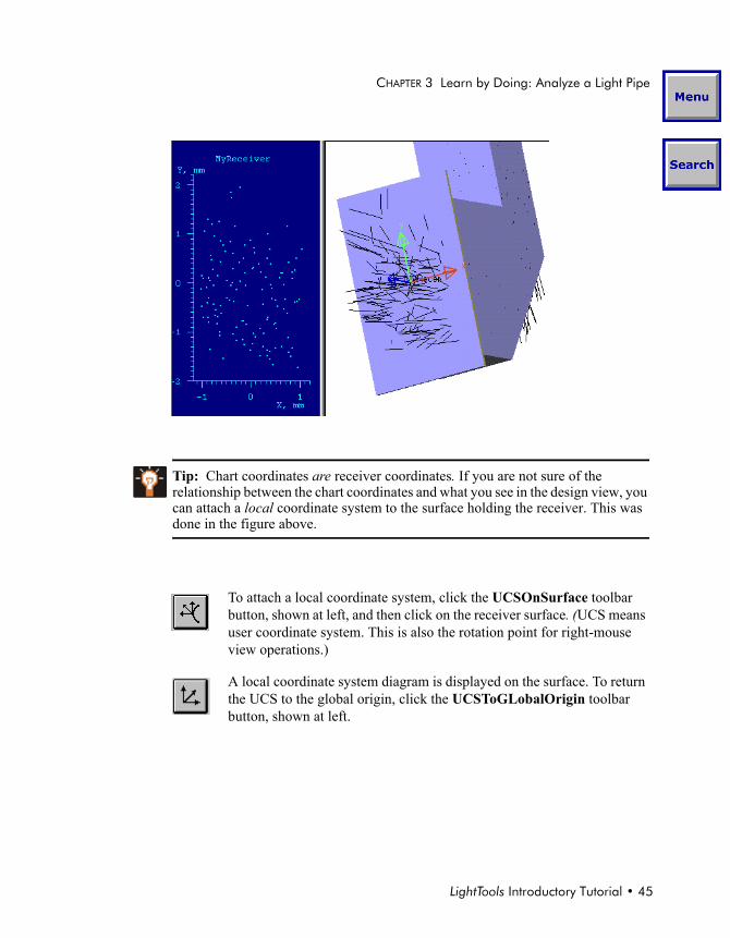
With only 200 rays for preview, the scatter chart is not very dense, but it can help you understand the relationship between chart coordinates and system coordinates. In the figure below, the 3D Design View has been rotated so that the receiver surface has the same orientation as the chart. You can see that the scatter chart is a kind of “ray diagram,” showing where the rays fall on the receiver surface.

Note: The menus always use the term illuminance, although, strictly speaking, this term applies only when photometric units are in use. In this example, the spatial distribution is in radiometric units of watts/mm2.



Tip: Chart coordinates are receiver coordinates. If you are not sure of the relationship between the chart coordinates and what you see in the design view, you can attach a local coordinate system to the surface holding the receiver. This was done in the figure above.

To attach a local coordinate system, click the UCSOnSurface toolbar button, shown at left, and then click on the receiver surface. (UCS means user coordinate system. This is also the rotation point for right-mouse view operations.)

A local coordinate system diagram is displayed on the surface. To return the UCS to the global origin, click the UCSToGLobalOrigin toolbar button, shown at left.



Making the Big RunIf the simulation with a few rays doesn't show any major problems, you can try a bigger run.

1. Click on the 3D Design View to make it active.

2. Select Illumination > Simulation Info to display the Illumination Simulation properties dialog box.

3. Change the Total Rays to Trace to 10000.

4. Uncheck the Preview Rays box (click the check box to clear it) and click OK.

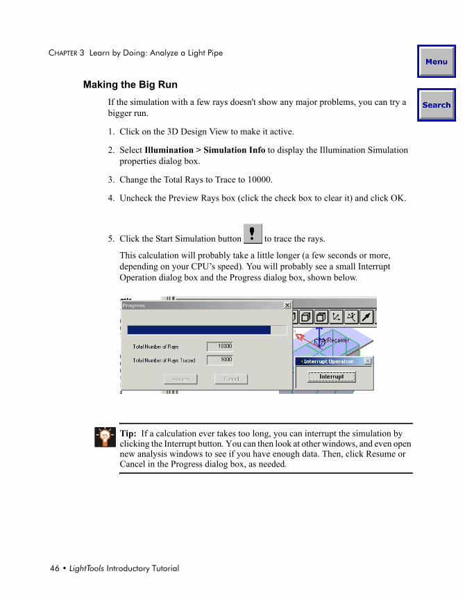
5. Click the Start Simulation button to trace the rays.

This calculation will probably take a little longer (a few seconds or more, depending on your CPU’s speed). You will probably see a small Interrupt Operation dialog box and the Progress dialog box, shown below.

Tip: If a calculation ever takes too long, you can interrupt the simulation by clicking the Interrupt button. You can then look at other windows, and even open new analysis windows to see if you have enough data. Then, click Resume or Cancel in the Progress dialog box, as needed.



Analysis Results and Re-binningAt this point, your scatter chart should be quite dense with rays. With more rays, illumination calculations make sense, so take a look at a pseudo-color raster chart of the illuminance (actually, irradiance, in this case, with units of W/mm2 and no photometric weighting. Please see Chapter 2 of the LightTools Illumination Module User’s Guide for information on radiometric vs. photometric calculations). To display a raster chart, make the design view the active window, and select Illumination > Illuminance Display > Raster Chart on the main menu.

The raster chart shows a pseudo-color coded, graphically smoothed map of irradiance (spatial) distribution on the receiver, along with a histogram showing the energy levels. You can see a fairly “hot” region in the center, with dark edges. How much data is here? How accurate is it? As with most objects in LightTools, receivers and charts have properties, and you can look to them to answer these questions.

1. Right-click near the center of the raster chart (on the shaded area).

The Properties dialog box for the Illumination Mesh_shade is displayed. Like other property dialog boxes, it has a small navigation tree. (You can also access mesh and other properties from the Illumination Manager section of the System Navigator, even if no charts are open.)



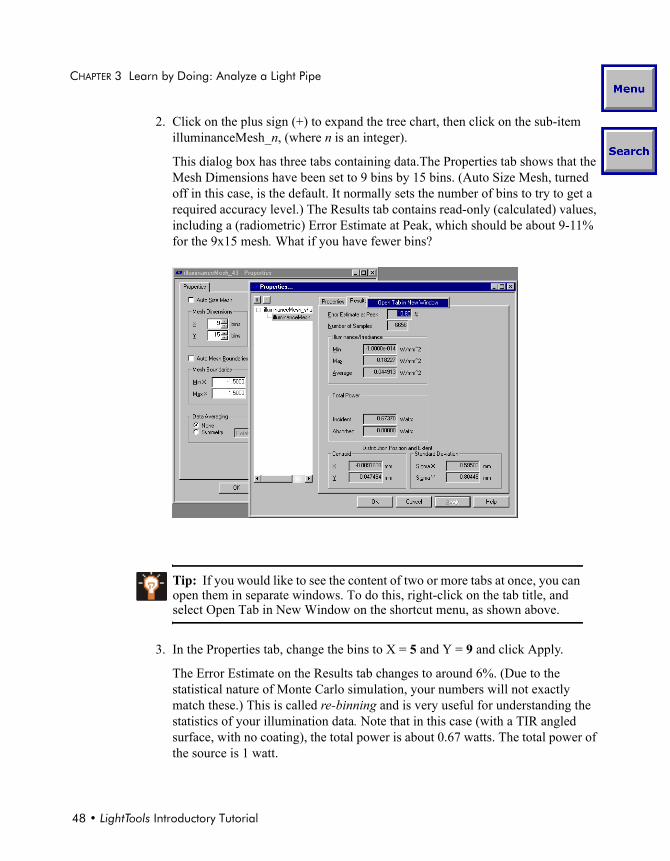
2. Click on the plus sign (+) to expand the tree chart, then click on the sub-item illuminanceMesh_n, (where n is an integer).

This dialog box has three tabs containing data.The Properties tab shows that the Mesh Dimensions have been set to 9 bins by 15 bins. (Auto Size Mesh, turned off in this case, is the default. It normally sets the number of bins to try to get a required accuracy level.) The Results tab contains read-only (calculated) values, including a (radiometric) Error Estimate at Peak, which should be about 9-11% for the 9x15 mesh. What if you have fewer bins?

3. In the Properties tab, change the bins to X = 5 and Y = 9 and click Apply.

The Error Estimate on the Results tab changes to around 6%. (Due to the statistical nature of Monte Carlo simulation, your numbers will not exactly match these.) This is called re-binning and is very useful for understanding the statistics of your illumination data. Note that in this case (with a TIR angled surface, with no coating), the total power is about 0.67 watts. The total power of the source is 1 watt.

Tip: If you would like to see the content of two or more tabs at once, you can open them in separate windows. To do this, right-click on the tab title, and select Open Tab in New Window on the shortcut menu, as shown above.



Optical Properties Example: Paint It WhiteTo improve the uniformity of illumination in this case, you could try a number of techniques: “stair-step” extrusions, a curved surface, patterns of paint dots, or 3D textures (bumps or grooves), for example.

One quick option to try is to paint it white. LightTools provides a number of pre-defined optical properties, including one called White Paint, in an easy-to-use library of properties. These library properties are created by combining several basic properties; for example, the White Paint property creates a Lambertian scatterer with 92% reflectance. You can, of course, set basic properties directly, and you can save and name your own combinations in .opr (for optical property) files.

1. In the 3D Design View, rotate the view so that you can click on the TIR_fold surface.

2. Right-click, and select Optical Properties on the shortcut menu.

The Properties dialog box is displayed, with the Optical Properties tab in the foreground.

3. Click the radio button for Load From Library.

4. Select Surface Finishes from the first drop-down list, shown in the following figure.



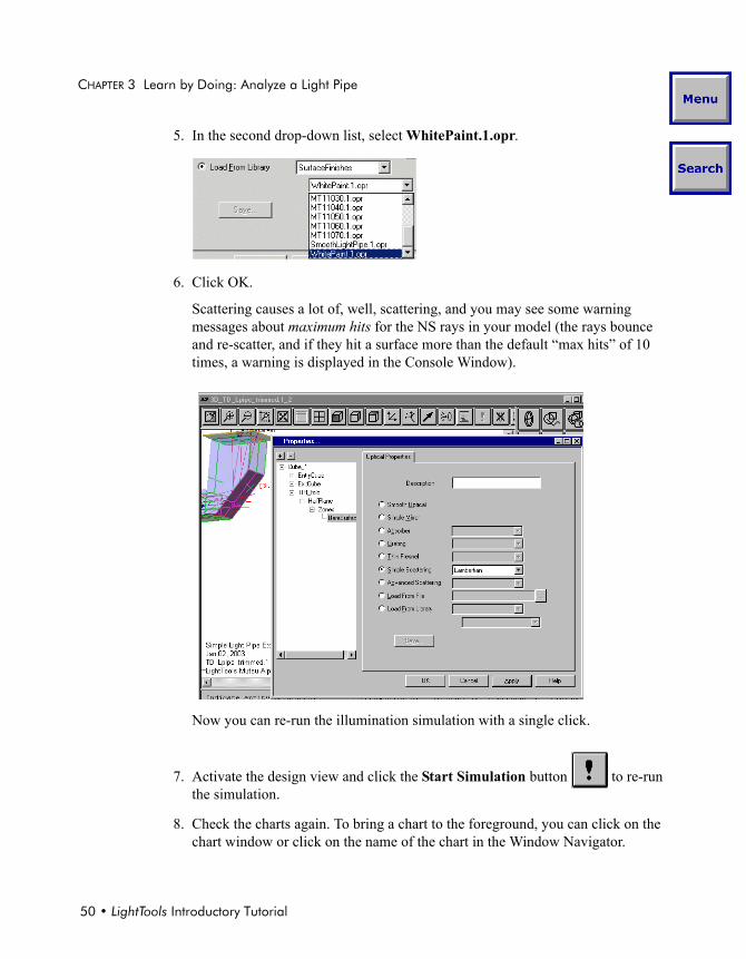
5. In the second drop-down list, select WhitePaint.1.opr.

6. Click OK.

Scattering causes a lot of, well, scattering, and you may see some warning messages about maximum hits for the NS rays in your model (the rays bounce and re-scatter, and if they hit a surface more than the default “max hits” of 10 times, a warning is displayed in the Console Window).

Now you can re-run the illumination simulation with a single click.

7. Activate the design view and click the Start Simulation button to re-run the simulation.

8. Check the charts again. To bring a chart to the foreground, you can click on the chart window or click on the name of the chart in the Window Navigator.



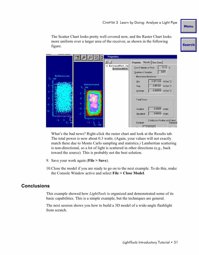
The Scatter Chart looks pretty well covered now, and the Raster Chart looks more uniform over a larger area of the receiver, as shown in the following figure.

What’s the bad news? Right-click the raster chart and look at the Results tab. The total power is now about 0.3 watts. (Again, your values will not exactly match these due to Monte Carlo sampling and statistics.) Lambertian scattering is non-directional, so a lot of light is scattered in other directions (e.g., back toward the source). This is probably not the best solution.

9. Save your work again (File > Save).

10.Close the model if you are ready to go on to the next example. To do this, make the Console Window active and select File > Close Model.

ConclusionsThis example showed how LightTools is organized and demonstrated some of its basic capabilities. This is a simple example, but the techniques are general.

The next session shows you how to build a 3D model of a wide-angle flashlight from scratch.

Documents

Chapter 3 Learn by Doing: Analyze a Light Pipe