Embed Size (px)
Citation preview

Chapter 3
Gradient-based optimization
Contents (class version)3.0 Introduction . . . . . . . . . . . . . . . . . . . . . . . . . . . . . . . . . . . . . . . . 3.3
3.1 Lipschitz continuity . . . . . . . . . . . . . . . . . . . . . . . . . . . . . . . . . . . . 3.6
3.2 Gradient descent for smooth convex functions . . . . . . . . . . . . . . . . . . . . . 3.14
3.3 Preconditioned steepest descent . . . . . . . . . . . . . . . . . . . . . . . . . . . . . 3.18Preconditioning: overview . . . . . . . . . . . . . . . . . . . . . . . . . . . . . . . . . . . . . 3.19
Descent direction . . . . . . . . . . . . . . . . . . . . . . . . . . . . . . . . . . . . . . . . . . 3.21
Complex case . . . . . . . . . . . . . . . . . . . . . . . . . . . . . . . . . . . . . . . . . . . . 3.22
3.4 Descent direction for edge-preserving regularizer: complex case . . . . . . . . . . . 3.23GD step size with preconditioning . . . . . . . . . . . . . . . . . . . . . . . . . . . . . . . . . 3.28
Finite difference implementation . . . . . . . . . . . . . . . . . . . . . . . . . . . . . . . . . . 3.29
Orthogonality for steepest descent and conjugate gradients . . . . . . . . . . . . . . . . . . . . 3.31
3.5 General inverse problems . . . . . . . . . . . . . . . . . . . . . . . . . . . . . . . . . 3.32
3.6 Convergence rates . . . . . . . . . . . . . . . . . . . . . . . . . . . . . . . . . . . . . 3.34Heavy ball method . . . . . . . . . . . . . . . . . . . . . . . . . . . . . . . . . . . . . . . . . 3.35
Generalized convergence analysis of PGD . . . . . . . . . . . . . . . . . . . . . . . . . . . . . 3.38
3.1

© J. Fessler, January 16, 2020, 17:44 (class version) 3.2
Generalized Nesterov fast gradient method (FGM) . . . . . . . . . . . . . . . . . . . . . . . . 3.40
3.7 First-order methods . . . . . . . . . . . . . . . . . . . . . . . . . . . . . . . . . . . . 3.41General first-order method classes . . . . . . . . . . . . . . . . . . . . . . . . . . . . . . . . . 3.41
Optimized gradient method (OGM) . . . . . . . . . . . . . . . . . . . . . . . . . . . . . . . . 3.45
3.8 Machine learning via logistic regression for binary classification . . . . . . . . . . . 3.52Adaptive restart of OGM . . . . . . . . . . . . . . . . . . . . . . . . . . . . . . . . . . . . . . 3.57
3.9 Summary . . . . . . . . . . . . . . . . . . . . . . . . . . . . . . . . . . . . . . . . . . 3.58

© J. Fessler, January 16, 2020, 17:44 (class version) 3.3
3.0 Introduction
To solve a problem likex = arg min
x∈FN
Ψ(x)
via an iterative method, we start with some initial guess x0, and then the algorithm produces a sequence {xt}where hopefully the sequence converges to x, meaning ‖xt − x‖ → 0 for some norm ‖·‖ as t→∞.
What algorithm we use depends greatly on the properties of the cost function Ψ : FN 7→ R.
EECS 551 explored the gradient descent (GD) and preconditioned gradient descent (PGD) algorithms forsolving least-squares problems in detail.
Here we review the general form of gradient descent (GD) for convex minimization problems; the LSapplication is simply a special case.
Venndiagram
forconvex
functions:
nonsmooth composite differentiableLipschitz
continuousgradient
twicedifferentiable
withboundedcurvature
quadratic(LS)

© J. Fessler, January 16, 2020, 17:44 (class version) 3.4
Motivating application(s)
We focus initially on the numerous SIPML applications where the cost function is convex and smooth,meaning it has a Lipschitz continuous gradient.
A concrete family of applications is edge-preserving image recovery where the measurement model is
y = Ax + ε
for some matrix A and we estimate x using
x = arg minx∈FN
1
2‖Ax− y‖2
2 + βR(x)
where the regularizer is convex and smooth, such as
R(x) =∑k
ψ([Cx]k)
for a potential function ψ that has a Lipschitz continuous derivative, such as the Fair potential.

© J. Fessler, January 16, 2020, 17:44 (class version) 3.5
Example. Here is an example of image deblurring or image restoration that was performed using such amethod. The left image is the blurry noisy image y, and the right image is the restored image x.
Step sizes and Lipschitz constant preview
For gradient-based optimization methods, a key issue is choosing an appropriate step size (aka learning ratein ML). Usually the appropriate range of step sizes is determined by the Lipschitz constant of ∇Ψ, so wefocus on that next.

© J. Fessler, January 16, 2020, 17:44 (class version) 3.6
3.1 Lipschitz continuity
The concept of Lipschitz continuity is defined for general metric spaces, but we focus on vector spaces.
Define. A function g : FN 7→ FM is Lipschitz continuous if there exists L < ∞, called a Lipschitzconstant, such that
‖g(x)− g(z)‖ ≤ L ‖x− z‖ , ∀x, z ∈ RN .
In general the norms on FN and FM can differ and L will depend on the choice of the norms. We will focuson the Euclidean norms unless otherwise specified.
Define. The smallest such L is called the best Lipschitz constant. (Often just “the” LC.)
Algebraic properties
Let f and g be Lipschitz continuous functions with (best) Lipschitz constants Lf and Lg respectively.
h(x) Lh
αf(x) + β |α|Lf scale/shiftf(x− x0) Lf translatef(x) + g(x) ≤ Lf + Lg addf(g(x)) ≤ LfLg compose ( HW )Ax + b |||A||| affine (for same norm on FM and FN )f(x)g(x) ? multiply

© J. Fessler, January 16, 2020, 17:44 (class version) 3.7
If f and g are Lipschitz continuous functions on R, then h(x) = f(x)g(x) is a Lipschitz continuousfunction on R. (?)A: True B: False ??
If f : FN 7→ F and g : FN 7→ F are Lipschitz continuous functions and h(x) , f(x)g(x),
and |f(x)| ≤ fmax <∞ and |g(x)| ≤ gmax <∞,
then h(·) is Lipschitz continuous on FN and Lh ≤ fmaxLg + gmaxLf .
Proof
|h(x)− h(z)| = |f(x)g(x)− f(z)g(z)|
= |f(x)(g(x)− g(z))− (f(z)− f(x))g(z)|
≤ |f(x)| |g(x)− g(z)|+ |g(z)| |f(x)− f(z)| by triangle ineq.
≤ (fmaxLg + gmaxLf ) ‖x− z‖2 . 2
Is boundedness of both f and g a necessary condition? group
No. Think f(x) = α and g(x) = x. Then Lfg = |α| = fmax but g(·) is unbounded yet Lipschitz.Think f(x) = g(x) =
√|x|, both unbounded. But h(x) = f(x)g(x) = |x| has Lh = 1.

© J. Fessler, January 16, 2020, 17:44 (class version) 3.8
For our purposes, we especially care about cost functions whose gradients are Lipschitz continuous. We callthese smooth functions. The definition of gradient is subtle for functions on CN so here we focus on RN .
Define. A differentiable function f(x) is called smooth iff it has a Lipschitz continuous gradient, i.e., iff∃L <∞ such that
‖∇f(x)−∇f(z)‖2 ≤ L ‖x− z‖2 , ∀x, z ∈ RN .
Lipschitz continuity of∇f is a stronger condition than mere continuity, so any differentiable function whosegradient is Lipschitz continuous is in fact a continuously differentiable function.
The set of differentiable functions on RN having L-Lipschitz continuous gradients is sometimes denotedC1,1L (RN) [1, p. 20].
Example. For f(x) = 12‖Ax− y‖2
2 we have ‖∇f(x)−∇f(z)‖2 = ‖A′(Ax− y)−A′(Az − y)‖2
= ‖A′A(x− z)‖2 ≤ |||A′A|||2 ‖x− z‖2 .So the Lipschitz constant of∇f is L∇f = |||A′A|||2 = |||A|||22 = σ2(A) = ρ(A′A).
The value L∇f = |||A′A|||2 is the best Lipschitz constant for ∇f(·). (?)A: True B: False ????

© J. Fessler, January 16, 2020, 17:44 (class version) 3.9
Here is an interesting geometric property of functions in C1,1L (RN) [1, p. 22, Lemma 1.2.3]:
|f(x)− f(z)−∇f(z)(x− z)| ≤ L
2‖x− z‖2
2 , ∀x, z ∈ RN .
In other words, for any point z, the function f(x) is bounded between the two quadratic functions:
q±(x) , f(z) + 〈∇f(z), x− z〉±L2‖x− z‖2
2 .
(Picture)of sinusoid sin(x) with bounding upward and downward parabolas.
Convex functions with Lipschitz continuous gradients
See [1, p. 56] for many equivalent conditions for a convex differentiable function f to have a Lipschitzcontinuous gradient, such as the following holding for all x, z ∈ RN :
f(z) + 〈∇f(z), x− z〉 ≤︸ ︷︷ ︸tangent plane property
f(x)≤ f(z) + 〈∇f(z), x− z〉+L2‖x− z‖2
2︸ ︷︷ ︸quadratic majorization property
. (Picture)
The left inequality holds for all differentiable convex functions.

© J. Fessler, January 16, 2020, 17:44 (class version) 3.10
Fact. If f(x) is twice differentiable and if there exists L <∞ such that its Hessian matrix has a boundedspectral norm: ∣∣∣∣∣∣∇2f(x)
∣∣∣∣∣∣2≤ L, ∀x ∈ RN , (3.1)
then f(x) has a Lipschitz continuous gradient with Lipschitz constant L.
So twice differentiability with bounded curvature is sufficient, but not necessary, for a function to haveLipschitz continuous gradient.
Proof. Using Taylor’s theorem and the triangle inequality and the definition of spectral norm:
‖∇f(x)−∇f(z)‖2 =
∥∥∥∥∫ 1
0
∇2f(x + τ(z − x)) dτ (x− z)
∥∥∥∥2
≤(∫ 1
0
∣∣∣∣∣∣∇2f(x + τ(z − x))∣∣∣∣∣∣
2dτ
)‖z − z‖2 ≤
(∫ 1
0
L dτ
)‖x− z‖2 = L ‖x− z‖2 .
Example. f(x) = 12‖Ax− y‖2
2 =⇒ ∇2f = A′A so |||∇2f |||2 = |||A′A|||2 = |||A|||22.
Example. The Lipschitz constant for the gradient of f(x) , x′[1 22 4
]x is:
∇2f = 2zz′ where z′ = [1 2] so |||∇2f |||2 = 2 ‖z‖22 = 10.
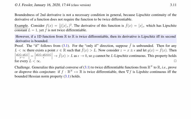
© J. Fessler, January 16, 2020, 17:44 (class version) 3.11
Boundedness of 2nd derivative is not a necessary condition in general, because Lipschitz continuity of thederivative of a function does not require the function to be twice differentiable.
Example. Consider f(x) = 12([x]+)2. The derivative of this function is f(x) = [x]+ which has Lipschitz
constant L = 1, yet f is not twice differentiable.
However, if a 1D function from R to R is twice differentiable, then its derivative is Lipschitz iff its secondderivative is bounded.
Proof. The “if” follows from (3.1). For the “only if” direction, suppose f is unbounded. Then for anyL < ∞ there exists a point x ∈ R such that f(x) > L. Now consider z = x ± ε and let g(x) = f(x). Then∣∣∣g(x)−g(z)
x−z
∣∣∣ =∣∣∣g(x)−g(x±ε)
ε
∣∣∣→ f(x) > L as ε→ 0, so g cannot be L-Lipschitz continuous. This property holdsfor every L <∞. 2
Challenge. Generalize this partial converse of (3.1) to twice differentiable functions from RN to R, i.e., proveor disprove this conjecture: if f : RN 7→ R is twice differentiable, then ∇f is Lipshitz continuous iff thebounded Hessian norm property (3.1) holds.

© J. Fessler, January 16, 2020, 17:44 (class version) 3.12
(Read)
Example. The Fair potential used in many imagingapplications [2] [3] is
ψ(z) = δ2 (|z/δ| − log(1 + |z/δ|)) , (3.2)
for some δ > 0 and has the property of being roughlyquadratic for z ≈ 0 and roughly like |z| for δ |z| � 0.When the domain of ψ is R, we can differentiate (care-fully treat z > 0 and z < 0 separately):
ψ(z) =z
1 + |z/δ|and ψ(z) =
1
(1 + |z/δ|)2≤ 1,
so the Lipschitz constant of the derivative of ψ(·) is 1.Furthermore, its second derivative is nonnegative so itis a convex function.In the figure, δ = 1.
-1 0 1 30
1
-1 0 1 3
-1
0
1
Example. Is the Fair potential ψ itself Lipschitz continuous? Yes:∣∣∣ψ(z)
∣∣∣ ≤ 1.

© J. Fessler, January 16, 2020, 17:44 (class version) 3.13
Edge-preserving regularizer and Lipschitz continuity
Example. Determine “the” Lipschitz constant for the gradient of the edge-preserving regularizer in RN ,when the derivative ψ of potential function ψ has Lipschitz constant Lψ :
R(x) =K∑k=1
ψ([Cx]k) =⇒ ∇R(x) = C ′ ψ .(Cx) = h(g(f(x))), (3.3)
where f(x) = Cx, g(u) = ψ .(u), h(v) = C ′v, Lf = |||C|||2, Lh = |||C ′|||2. (students finish it)
‖g(u)− g(v)‖22 =
∥∥∥ψ .(u)− ψ .(v)∥∥∥2
2=∑k
∣∣∣ψ(uk)− ψ(vk)∣∣∣2 ≤∑
k
L2ψ|uk − vk|2 = L2
ψ‖u− v‖2
2
=⇒ Lg ≤ Lψ, =⇒ L∇R ≤ Lψ|||C|||22 = Lψ|||C ′C|||2. (3.4)
Thus when ψ ≤ 1, a Lipschitz constant for the gradient of the above R(x) is:A: 1 B: |||C|||2 C: |||C ′C|||2 D: |||C|||42 E: None of these ??
Showing this L∇R is the best Lipschitz constant is a HW problem.
© J. Fessler, January 16, 2020, 17:44 (class version) 3.14
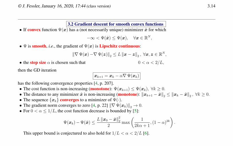
3.2 Gradient descent for smooth convex functions• If convex function Ψ(x) has a (not necessarily unique) minimizer x for which
−∞ < Ψ(x) ≤ Ψ(x), ∀x ∈ RN ,
• Ψ is smooth, i.e., the gradient of Ψ(x) is Lipschitz continuous:
‖∇Ψ(x)−∇Ψ(z)‖2 ≤ L ‖x− z‖2 , ∀x, z ∈ RN ,
• the step size α is chosen such that 0 < α < 2/L,
then the GD iterationxk+1 = xk − α∇Ψ(xk)
has the following convergence properties [4, p. 207].• The cost function is non-increasing (monotone): Ψ(xk+1) ≤ Ψ(xk), ∀k ≥ 0.• The distance to any minimizer x is non-increasing (monotone): ‖xk+1 − x‖2 ≤ ‖xk − x‖2 , ∀k ≥ 0.• The sequence {xk} converges to a minimizer of Ψ(·).• The gradient norm converges to zero [4, p. 22] ‖∇Ψ(xk)‖2 → 0.• For 0 < α ≤ 1/L, the cost function decrease is bounded by [5]:
Ψ(xk)−Ψ(x) ≤ L ‖x0 − x‖22
2max
(1
2kα + 1, (1− α)2k
).
This upper bound is conjectured to also hold for 1/L < α < 2/L [6].

© J. Fessler, January 16, 2020, 17:44 (class version) 3.15
Optimal asymptotic step size for GD (Read)
The above step size range 0 < α < 2/L is a wide range of values, and one might ask what is the best choice?
For a LS cost function f(x) = 12‖Ax− y‖2
2 , the EECS 551 notes show that the asymptotically optimalchoice of the step size is:
α∗ =2
σmax(A′A) + σmin(A′A)=
2
σmax(∇2f) + σmin(∇2f),
because ∇2f = A′A.
For more general cost functions that are twice differentiable, one can apply similar analyses to show that theasymptotically optimal choice is
α∗ =2
σmax(∇2f(x)) + σmin(∇2f(x)).
Although this formula is an interesting generalization, it is of little practical use because we do not know theminimizer x and the Hessian∇2f and its SVD are infeasible for large problems.Furthermore, the asymptotically optimal choice of α∗ may not be the best step size in the early iterationswhen the iterates are far from x.

© J. Fessler, January 16, 2020, 17:44 (class version) 3.16
Convergence rates (Read)
There are many ways to assess the convergence rate of an iterative algorithm like GD. Researchers study:
• Ψ(xk)→ Ψ(x)• ‖∇Ψ(xk)‖ → 0• ‖xk − x‖ → 0
both globally and locally...
Ψ(x)
xxk x
Ψ(x)
Ψ(xk)
‖xk − x‖
‖∇Ψ(xk)‖
Quantifying bounds on the rates of decrease of these quantities is an active research area. Even classical GDhas relatively recent results [5] that tighten up the traditional bounds. The tightest possible worst-case boundfor GD for the decrease of the cost function (with a fixed step size α = 1/L) is O(1/k):
Ψ(xk)−Ψ(x) ≤ ‖x0 − x‖22
L (4k + 2),
where L is the Lipschitz constant of the gradient∇f(x).
In contrast, Nesterov’s fast gradient method (p. 3.40) has a worst-case cost function decrease at rate at leastO(1/k2), which can be improved (and has) by only a constant factor [7].

© J. Fessler, January 16, 2020, 17:44 (class version) 3.17
Example. The following figure illustrates how slow GD can converge for a simple LS problem
with A =
[1 00 2
]and y = 0. This case used the optimal step size α∗ for illustration.
This slow convergence has been the impetus of thousands of papers on faster algorithms!
-4 -3 -2 -1 0-1
0
1
1
2
3
4
5
1
2
3
4
5
GD
The ellipses show the contours of the LS cost function ‖Ax− y‖ .
Two ways to try to accelerate convergence are to use a preconditioner and/or a line search.

© J. Fessler, January 16, 2020, 17:44 (class version) 3.18
3.3 Preconditioned steepest descent (Read)
Instead of using GD with a fixed step size α, an alternative is to do a line search to find the best step sizeat each iteration. This variation is called steepest descent (or GD with a line search) [8]. Here is howpreconditioned steepest descent for a linear LS problem works:
dk = −P ∇Ψ(xk) search direction (negative preconditioned gradient)αk = arg min
αΨ(xk + αdk) step size
xk+1 = xk + αkdk update.
• Finding αk analytically quadratic cases is a HW problem• By construction, this iteration is guaranteed to decrease the cost function monotonically, with strict de-
crease unless xk is already a minimizer, provided the preconditioner P is positive definite. Expressedmathematically:
∇Ψ(xk) 6= 0 =⇒ Ψ(xk+1) < Ψ(xk) .
• Computing αk takes some extra work, especially for non-quadratic problems. Often Nesterov’s fast gra-dient method or the optimized gradient method (OGM) [7] are preferable because they do not require aline search (if the Lipschitz constant is available).

© J. Fessler, January 16, 2020, 17:44 (class version) 3.19
Preconditioning: overview (Read)
Why use the preconditioned search direction dk = −P∇Ψ(xk) ?
Consider the least-squares cost function Ψ(x) = 12‖Ax− y‖2
2 , and define a “preconditioned” cost functionusing a change of coordinates:
f(z) , Ψ(Tz) =1
2‖ATz − y‖2
2 .
The Hessian matrix of f(·) is ∇2f(z) = T ′A′AT .Applying GD to f yields
zk+1 = zk − α∇f(zk) = T ′A′(A′Tzk − y)
=⇒ Tzk+1 = Tzk − αTT ′A′(A′Tzk − y)
=⇒ xk+1 = xk − αPA′(A′xk − y) = xk − αP∇Ψ(xk),
where xk , T zk and P , TT ′. So ordinary GD on f is the same as preconditioned GD on Ψ.
If α = 1 and T = (A′A)−1/2, then P = (A′A)−1 and x1 = (A′A)−1A′y.In this sense P = (A′A)−1 = [∇2 Ψ(xk)]
−1 is the ideal preconditioner.

© J. Fessler, January 16, 2020, 17:44 (class version) 3.20
To elaborate, when T = (A′A)−1/2, then f(z) simplifies as follows:
f(z) =1
2(ATz − y)′(ATz − y) =
1
2
(z′T ′A′ATz − 2 real{y′ATz}+ ‖y‖2
2
)=
1
2
(z′Iz − 2 real{y′ATz}+ ‖y‖2
2
)=
1
2
(‖z − T ′A′y‖2
2 − ‖T′A′y‖2
2 + ‖y‖22
).
The next figures illustrate this property of converging in 1 iteration for a quadratic cost with the ideal precon-ditioner.
Example. Effect of ideal preconditioner on quadratic cost function contours.
Contours of Ψ(x) contours of f(z)
use z0 and z∗

© J. Fessler, January 16, 2020, 17:44 (class version) 3.21
Descent direction
Define. A vector d ∈ FN descent direction for a cost function Ψ : FN 7→ R at a point x iff moving locallyfrom x along the direction d decreases the cost, i.e., (1D Picture)
∃ c = c(x,d,Ψ) > 0 s.t. ∀ε ∈ [0, c) Ψ(x + εd) ≤ Ψ(x) . (3.5)
With this definition d = 0 is always a (degenerate) descent direction.
Fact. For RN , if Ψ(x) is differentiable at x and P is positive definite, then the following vector, if nonzero,is a descent direction for Ψ at x:
d = −P∇Ψ(x) . (3.6)
Proof sketch. Taylor’s theorem yields (Read)
Ψ(x)−Ψ(x + αd) = −α 〈∇Ψ(x), d〉+o(α) = α
[d′P−1d +
o(α)
α
],
which will be positive for sufficiently small α, because d′P−1d > 0 for P � 0, and o(α)/α→ 0 as α→ 0.
From this analysis we can see that designing/selecting a preconditioner that is positive definite is crucial.The two most common choices are:• P is diagonal with positive diagonal elements,• P = QDQ′ where D is diagonal with positive diagonal elements and Q is unitary.
In this case Q is often circulant so we can use FFT operations to perform Pg efficiently.

© J. Fessler, January 16, 2020, 17:44 (class version) 3.22
Complex case (Read)
The definition of descent direction in (3.5) is perfectly appropriate for both RN and CN . However, thedirection d specified in (3.6) is problematic in general on FN because many cost functions of interest are notholomorphic so are not differentiable on FN .
However, despite not being differentiable, we can still find a descent direction for most cases of interest.
Example. The most important case of interest here is Ψ : CN 7→ R defined by Ψ(x) = 12‖Ax− y‖2
2 whereA ∈ CM×N and y ∈ CM . This function is not holomorphic. However, one can show that
d = −PA′(Ax− y)
is a descent direction for Ψ at x when P is a positive definite matrix. ( HW )
In the context of optimization problems, when we write g = ∇Ψ(x) = A′(Ax − y) for the complex case,we mean that −g is a descent direction for Ψ at x, not a derivative.
Furthermore, one can show ( HW ) that the set of minimizers of Ψ(x) is the same as the set of points thatsatisfy ∇Ψ(x) = A′(Ax − y) = 0. So again even though a derivative is not defined here, the descentdirection sure walks like a duck and talks like a duck, I mean like a (negated) derivative.

© J. Fessler, January 16, 2020, 17:44 (class version) 3.23
3.4 Descent direction for edge-preserving regularizer: complex case
Now consider an edge-preserving regularizer defined on CN :
R(x) =K∑k=1
ψ([Cx]k), where ψ(z) = f(|z|) (3.7)
for some some potential function ψ : C 7→ R defined in terms of some function f : R 7→ R.
If f(r) = r2 then it follows from p. 3.22 that C ′Cx is a descent direction for R(x) on CN .But it seems unclear in general how to define a descent direction, due to the |·| above.
To proceed, make the following assumptions about the function f :• f : R 7→ R.• 0 ≤ s ≤ t =⇒ f(s) ≤ f(t) (monotone).• f is differentiable on R.
• ωf (t) ,f(t)
tis well-defined for all t ∈ R, including t = 0.
• 0 ≤ ωf (t) ≤ ωmax <∞.Example. For the Fair potential ωf (t) = 1/ (1 + |t/δ|) ∈ (0, 1].

© J. Fessler, January 16, 2020, 17:44 (class version) 3.24
Claim. For these assumptions, a descent direction for the edge-preserving regularizer (3.7) for x ∈ FN is
−∇R(x) = −C ′ diag{ωf .(|Cx|)}Cx, (3.8)
where the |·| is evaluated element-wise, like abs.() in JULIA. Intuition: f(t) = ωf (t) t.
To prove this claim, we focus on just one term in the sum: (Read)
r(x) , ψ(v′x) = f(|v′x|), d(x) = −v ωf (|v′x|)v′x.
for some nonzero vector v ∈ CN . (A row of C in (3.7) corresponds to v′.)
Letting ω = ωf (|v′x|) ≤ ωmax we have
r(x + εd) = f(|v′(x + εd)|) = f(|v′(x− εωvv′x)|) = f(|v′x(1− εωv′v)|) = f(|v′x|
∣∣1− εω ‖v‖22
∣∣).Now when 0 ≤ ε ≤ 1/(ω ‖v‖2
2) then∣∣1− εω ‖v‖22
∣∣ = 1− εω ‖v‖22 ∈ [0, 1],
=⇒ r(x + εd) = f(|v′x|
(1− εω ‖v‖2
2
))≤ f(|v′x|) = r(x),
using the monotone property of f(·). So d(x) is a descent direction for r(x).The proof of (3.8) involves the sum of K such terms. 2

© J. Fessler, January 16, 2020, 17:44 (class version) 3.25
So with our usual reuse of ∇ to denote a (negated) descent direction, we will not write (3.3) for CN butrather we will define ωψ = ωf and write:
∇R(x) = C ′ diag{ωψ .(|Cx|)}Cx. (3.9)
If ψ(z) = ψ(|z|), ∀z ∈ C, then we can define ωψ in terms of ψ for nonnegative real arguments.
The result (3.9) is shown in [9] using Wirtinger calculus.

© J. Fessler, January 16, 2020, 17:44 (class version) 3.26
Lipschitz constant for descent direction (Read)
Having established the descent direction (3.8) for edge-preserving regularization on CN , the next step is todetermine a Lipschitz constant for that function.
Again we can write it as a composition of three functions:
C ′ diag{ωψ .(|Cx|)}Cx = h(g(f(x))), f(x) = Cx, g(u) = d.(u), h(v) = C ′v, d(z) , ωψ(|z|) z.
For real z arguments and when ψ and hence ωψ are symmetric, d(z) = ψ(z) so the Lipschitz constant is easy.
When z ∈ C, I have not yet been able to prove Lipschitz continuity of d(z). My conjecture, supported bynumerical experiments and [9, App. A], is that if ωψ(t) is a non-increasing function of t on [0,∞), in additionto the other assumptions on p. 3.23, then
Ld = ωψ(0) (3.10)
and, akin to (3.4), the Lipschitz constant for the descent direction on CN is:
L∇R = |||C|||22Ld. (3.11)
Challenge. Prove (3.10). Here are some initial steps that might help:
|d(x)− d(z)| = |ωψ(|x|)x− ωψ(|z|) z| =∣∣ωψ(|x|) |x| eı∠x − ωψ(|z|) |z| eı∠z
∣∣=∣∣∣ψ(|x|) eı∠x − ψ(|z|) eı∠z
∣∣∣ ≤ ? ≤ ωψ(0) |x− z| .

© J. Fessler, January 16, 2020, 17:44 (class version) 3.27
Practical Lipschitz constant (Read)
In general, computing |||C|||22 in (3.4) exactly would require a SVD or the power iteration, both of which areimpractical for large-scale problems.
If we use finite differences with periodic boundary conditions, then C is circulant and hence is a normalmatrix so |||C|||2 = ρ(C), where ρ(·) denotes the spectra radius. For 1D finite differences with N even, thespectral radius is 2 and for N odd is 1 + cos(π(N − 1) /N) ≈ 2. ( HW )
But for nonperiodic boundary conditions we need a different approach.
Recall that because C ′C is symmetric:
|||C|||22 = |||C ′C|||2 = σ1(C ′C) = ρ(C ′C) ≤ |||C ′C|||,
for any matrix norm |||·|||. In particular, the matrix 1-norm is convenient:
|||C ′C|||1 ≤ |||C′|||1|||C|||1 = |||C|||∞|||C|||1
=⇒ |||C|||22 ≤ |||C|||∞|||C|||1 = 2 · 2 = 4
for 1D finite differences, because there as most a single +1 and −1 in each row or column of C.Interestingly, this 1-norm approach gives us an upper bound on |||C|||22 for any boundary conditions thatmatches the exact value when using periodic boundary conditions.
So the practical choice for 1D first-order finite-differences is to use L∇R = 4Lψ, where often we scale thepotential functions so thatLψ = 1.Bottom line: never use opnorm() when working with finite differences!

© J. Fessler, January 16, 2020, 17:44 (class version) 3.28
GD step size with preconditioning
We earlier argued that the preconditioned gradient −P∇Ψ(x) can be preferable to −∇Ψ(x) as a descentdirection. But the GD convergence theorem on p. 3.14 had no P in it. So must we resort to PSD on p. 3.18that requires a line search? No!
Suppose Ψ is convex has a Lipschitz continuous gradient with Lipschitz constant L∇Ψ.Define a new function in transformed coordinate system: f(z) , Ψ(Tz) . Using the properties on p. 3.6, thisfunction also has a Lipschitz continuous gradient and
∇f(z) = T ′∇Ψ(Tz) =⇒ L∇f ≤ |||T ′T |||2L∇Ψ.
Choose a step size 0 < αf < 2/L∇f for applying GD to f , yielding
zk+1 = zk − αf∇f(zk) = zk − αfT ′∇Ψ(Tzk)
=⇒ Tzk+1 = Tzk − αfTT ′∇Ψ(Tzk)
=⇒ xk+1 = xk − αfP∇Ψ(xk),
where xk , T zk and P = TT ′. So ordinary GD on f is the same as preconditioned GD on Ψ. The step sizeshould satisfy 0 < αf < 2/L∇f so it suffices (but can be suboptimal; see HW ) to choose
0 < αf <2
|||T ′T |||2L∇Ψ
=1
|||P |||22
L∇Ψ
.

© J. Fessler, January 16, 2020, 17:44 (class version) 3.29
Finite difference implementation
For x ∈ FN we need to compute first-order finite differences dn = xn+1 − xn, n = 1, . . . , N − 1,which in matrix notation is d = Cx ∈ FN−1. Here are eight (!) different implementations in JULIA:
function loopdiff(x::AbstractVector)N = length(x)y = similar(x, N-1)for n=1:(N-1)
@inbounds y[n] = x[n+1] - x[n]endreturn y
end
d = diff(x) # built-ind = loopdiff(x)d = (circshift(x, -1) - x)[1:(N-1)]d = [x[n+1]-x[n] for n=1:(length(x)-1)] # comprehensiond = @views x[2:end] - x[1:(end-1)] # indexingd = conv(x, eltype(x).([1, -1]))[2:end-1] # using DSPd = diagm(0 => -ones(N-1), 1 => ones(N-1))[1:(N-1),:] * x # big/slowd = spdiagm(0 => -ones(N-1), 1 => ones(N-1))[1:(N-1),:] * x # SparseArrays

© J. Fessler, January 16, 2020, 17:44 (class version) 3.30
Which is fastest? https://web.eecs.umich.edu/~fessler/course/598/demo/diff1.html
Use notebook to discuss@inbounds@viewsspdiagm (column-wise storage...)LinearMaps (cf fatrix in MIRT)
Adjoint tests
y′(Ax) = (A′y)′x or equivalently 〈Ax, y〉 = 〈x, A′y〉
x = randn(N); y = randn(M);
@assert isapprox(y’*(A*x), (A’*y)’*x)
A generalization of transpose for linear maps is called the adjoint.

© J. Fessler, January 16, 2020, 17:44 (class version) 3.31
Orthogonality for steepest descent and conjugate gradients
Recall that the (preconditioned) steepest descent method has three steps:• Descent direction dk, e.g., dk = −P∇Ψ(xk)• line search: αk = arg minα fk(α), fk(α) = Ψ(xk + αdk)• update xk+1 = xk + αkdk
By construction:0 = fk(αk) = 〈dk, ∇Ψ(xk + αkdk)〉 = 〈dk, ∇Ψ(xk+1)〉 .
In other words, the gradient∇Ψ(xk+1) at the next iterate is perpendicular to the current search direction dk:
dk ⊥ ∇Ψ(xk+1) .
This orthogonality leads to the “zig-zag” nature of PSD iterates seen on p. 3.17.
The preconditioned conjugate gradient (CG) method, described in more detail in [10], replaces the standardinner product with a different inner product weighted by the Hessian of the cost function:
〈dk, ∇Ψ(xk+1)〉H = d′kH∇Ψ(xk+1), H = ∇2 Ψ(xk),
leading to faster convergence. See [10] for details.
Note that the CG method we want for optimization is the nonlinear conjugate gradient (NCG) method; in �
these notes CG means NCG.

© J. Fessler, January 16, 2020, 17:44 (class version) 3.32
3.5 General inverse problems
As mentioned previously, a typical cost function for solving inverse problems has the form
x = arg minx∈FN
1
2‖Ax− y‖2
2 + βR(x), R(x) =K∑k=1
ψ([Cx]k) = r(Cx), r(v) =K∑k=1
ψ(vk) . (3.12)
This is just one of many possible special cases of the following fairly general form
Ψ(x) =J∑j=1
fj(Bjx) =⇒ ∇Ψ(x) =J∑j=1
B′j∇fj(Bjx), (3.13)
where Bj is a Mj ×N matrix and each fj : RMj 7→ R is a (typically convex) function.
Example. For the special case (3.12), we use (3.13) with
J = 2, B1 = A, B2 = C, f1(u) =1
2‖u− y‖2
2 , f2(v) = βr(v).
We will implement several algorithms for minimize cost functions of this general form.
When ψ is the Fair potential, the (best) Lipschitz constant of ∇f2(v) is:A: 1 B: β C: β
√K D: βK E: None ??

© J. Fessler, January 16, 2020, 17:44 (class version) 3.33
Efficient line search (Read)
A naive implementation of the line search step in the PSD algorithm on p. 3.18 minimizes
hk(α) , Ψ(xk + αdk) .
When applied to a cost function of the general form (3.13) this would involve repeated matrix-vector multi-plications of the form Bj(xk + αdk), which is expensive. A more efficient approach is to precompute thematrix-vector products prior to performing the line search, noting that for the general (3.13) form:
hk(α) = Ψ(xk + αdk) =J∑j=1
fj(Bj (xk + αdk)) =J∑j=1
fj
(u
(k)j + αv
(k)j
), u
(k)j , Bjxk, v
(k)j , Bjdk.
Precomputing u(k)j and v
(k)j prior to performing the line search avoids redundant matrix-vector products.
Furthermore, algorithms with line searches like PSD and PCG have an recursive update of the form:
xk+1 = xk + αkdk.
Multiplying both sides by Bj yields an efficient recursive update for the uj vector (used in HW problems):
Bjxk+1 = Bjxk + αkBjdk =⇒ u(k+1)j = u
(k)j + αv
(k)j .
A key simplification here is that the Lipschitz constant of hk does not use operator norms of any Bj . ( HW )

© J. Fessler, January 16, 2020, 17:44 (class version) 3.34
3.6 Convergence rates
Asymptotic convergence rates
When the cost function Ψ is locally strictly convex and twice differentiable near minimizer x, one can analyzethe asymptotic convergence rates of PGD, PSD, and PCG. (See Fessler book Ch. 11.)
All three algorithms satsify inequalities of the following form for different values of c, ρ:∥∥P−1/2(xk+1 − x)∥∥
2≤ cρk
∥∥P−1/2(x0 − x)∥∥
2=⇒ lim
k→∞
∥∥P−1/2(xk − x)∥∥1/k
2≤ ρ.
PGD and PSD produce sequences {xk} that con-verge linearly [1, p. 32] to x and
supx0
limk→∞
∥∥P−1/2(xk − x)∥∥1/k
2= ρ,
where ρ is called the root convergence factor.Define H = P 1/2∇2 Ψ(x)P 1/2 and conditionnumber κ = σ1(H)/σN(H).This table shows the values of ρ.
Method ρ κ = 102
PGD standard step α =1
σ1(H)
κ− 1
κ0.99
PGD α∗ =2
σ1(H) + σN(H)
κ− 1
κ+ 10.98
PSD with perfect line searchκ− 1
κ+ 10.98
PCG with perfect line search√κ− 1√κ+ 1
0.82
PCG converges quadratically [1, p. 45] and its ρ above matches a lower bound [1, p. 68].

© J. Fessler, January 16, 2020, 17:44 (class version) 3.35
Heavy ball method
One way to seek faster convergence is to use algorithms that have momentum.An early momentum method is the heavy ball method [4, p. 64]. One way to write it is:
dk = −∇Ψ(xk) +βkdk−1
xk+1 = xk + αkdk,
where αk > 0 and βk ≥ 0. The “search direction” dk depends on both the gradient and the previous direction.Rearranging the 2nd equation to write dk = (xk+1 − xk)/αk and the combining yields this form
xk+1 = xk − αk∇Ψ(xk)︸ ︷︷ ︸usual GD
+ βk (xk − xk−1)︸ ︷︷ ︸momentum
, βk , βkαkαk−1
. (3.14)
Convergence rate analysis (Read)
To analyze the convergence rate of this method we make two simplifications.• We consider the case of constant step sizes αk = α and βk = β = βk• We focus on a quadratic cost function Ψ(x) = 1
2‖Ax− y‖2
2 where M × N A has full column rank,so there is a unique minimizer x. Note that ∇Ψ(x) = A′(Ax − y) = Hx − b, where the Hessian isH = A′A and b = A′y. The unique minimizer satisfies the normal equations: Hx = b, so ∇Ψ(x) =Hx−Hx = H(x− x).

© J. Fessler, January 16, 2020, 17:44 (class version) 3.36
EECS 551 analyzed the convergence rate of GD by relating xk+1 − x to xk − x. Here the recursion (3.14)depends on both xk and xk−1 so we analyze the following two-state recursion:[xk+1 − xxk − x
]=
[xk − α∇Ψ(xk) +β(xk − xk−1)− x
xk − x
]=
[xk − x− αH(xk − x) + β(xk − xk−1)
xk − x
]=
[xk − x− αH(xk − x) + β(xk − x)− β(xk−1 − x)
xk − x
]= G
[xk − xxk−1 − x
], G ,
[(1 + β)I − αH βI
I 0
].
Because H is Hermitian, it has a unitary eigendecomposition H = V ΛV ′, with eigenvalues λi(H) =σ2i (A). Writing the governing matrix G using this eigendecomposition:
G =
[V 00 V
] [(1 + β)I − αΛ βI
I 0
] [V 00 V
]′(diagonal blocks)
=
[V 00 V
]Π
G1 0. . .
0 GN
Π′[V 00 V
]′, Gi =
[1 + β − αλi β
1 0
],
where Π is a 2N × 2N permutation matrix. Thus eig{G} = ∪Ni=1 eig{Gi}, using several eigenvalue proper-ties. The eigenvalues of Gi are the roots of its characteristic polynomial:
z2 − (1 + β − αλi)z + β.

© J. Fessler, January 16, 2020, 17:44 (class version) 3.37
If β = 0 then the nontrivial root is at z = 1− αλi, which is an expression see in the EECS 551 notes.
Otherwise the roots (eigenvalues of Gi) are:
z =(1 + β − αλi)±
√(1 + β − αλi)2 − 4β
2.
For the fastest convergence, we would like to choose α and β to minimize maxi ρ(Gi). One can show thatthe best choice is:
α∗ =4
(σ1(A) + σN(A))2, β∗ =
σ1(A)− σN(A)
σ1(A) + σN(A).
For this choice, one can show that
ρ(G) = β∗ =σ1(A)− σN(A)
σ1(A) + σN(A)=
√κ− 1√κ+ 1
,
where κ = σ1(H)/σN(H) = σ21(A)/σ2
N(A).
Thus for the simple LS problem, the heavy ball method with its best choice of step-size parameters has thesame rate as the conjugate gradient method with a perfect line search.
Of course in practice it is usually too expensive to determine σ1(A) and σN(A), so we next seek morepractical momentum methods that do not require these values.

© J. Fessler, January 16, 2020, 17:44 (class version) 3.38
Generalized convergence analysis of PGD
Define. The gradient of Ψ is S-Lipschitz continuous on RN for an invertible matrix S iff∥∥S−1 (∇Ψ(x)−∇Ψ(z))∥∥
2≤ ‖S′ (x− z)‖2 , ∀x, z ∈ RN . (3.15)
If S =√LI , then the S-Lipschitz condition (3.15) simplifies to the classic Lipschitz continuity condition:
‖∇Ψ(x)−∇Ψ(z)‖2 ≤ L‖x− z‖2 , ∀x, z ∈ RN . (3.16)
Theorem (PGD convergence). If∇Ψ satisfies (3.15) and for some 0 < α
αP ′SS′P ≺ P + P ′, (3.17)
then (i) the PGD algorithmxk+1 = xk − αP∇Ψ(xk) (3.18)
monotonically decreases Ψ [10] because for g = ∇Ψ(xk):
Ψ(xk)−Ψ(xk+1) ≥ α
2g′ (P + P ′ − αP ′SS′P ) g,
and (ii) ‖∇Ψ(xk)‖ → 0.

© J. Fessler, January 16, 2020, 17:44 (class version) 3.39
In the usual case where P is symmetric positive definite, (3.17) simplifies to αSS′ ≺ 2P−1 and when thatcondition holds then
∥∥P−1/2(xk − x)∥∥
2converges monotonically to zero [10].
If we choose αP = (SS′)−1, then PGD is equivalent to a majorize-minimize (MM) method (discussedlater) and the cost function decrease has the following bound:
Ψ(xk)−Ψ(x) ≤ ‖S′ (x0 − x)‖2
2k, k ≥ 1. (3.19)
The bound above is the “classical” textbook formula. In 2014 the following tight bound was found [5]:
Ψ(xk)−Ψ(x) ≤ ‖S′ (x0 − x)‖2
4k + 2, k ≥ 1. (3.20)
It is tight because there is a Huber-like function Ψ for which GD meets that rate.
Why generalize? Units of Lipschitz constant
Consider Ψ(x) = 12‖Ax− y‖2
2 where A is 2×2 diagonal with units:a11 ampere x1 ohm y1 volta22 volt/m x2 m y2 volt
What are the units of the Lipschitz constant of ∇Ψ?A: ampere volt / m B: ampere2 C: volt2 / m2 D: ohm m E: none of these ??

© J. Fessler, January 16, 2020, 17:44 (class version) 3.40
Generalized Nesterov fast gradient method (FGM)
The following is a slight generalization of the fast gradient method (FGM) of Nesterov, also known asaccelerated gradient descent and Nesterov accelerated gradient (NAG):Initialize t0 = 1 and z0 = x0 then for k = 0, 1, . . .:
tk+1 =
(1 +
√1 + 4t2k
)/2
xk+1 = zk − [SS′]−1∇Ψ(zk) gradient step
zk+1 = xk+1 +tk − 1
tk+1
(xk+1 − xk) . momentum
If tk = 1 for all k then FGM reverts to ordinary GD.
Theorem If Ψ is convex and has an S-Lipschitz gradient, then this generalized FGM satisfies:
Ψ(xk)−Ψ(x) ≤ 2 ‖S′ (x0 − x)‖2
k2. (3.21)
In words, the worst-case rate of decrease of the cost function Ψ is O(1/k2).This is a huge improvement over the O(1/k) rate of PGD in (3.19).However, worst-case analysis may be pessimistic for your favorite application.For example, if Ψ is quadratic on RN , then CG converges in N iterations.

© J. Fessler, January 16, 2020, 17:44 (class version) 3.41
3.7 First-order methods
The most famous second-order method is Newton’s method:
xk+1 = xk − (∇2 Ψ(xk))−1∇Ψ(xk) .
This method is impractical for large-scale problems so we focus on first-order methods [1, p. 7].
General first-order method classes• General first-order (GFO) method:
xk+1 = function(x0,Ψ(x0),∇Ψ(x0), . . . ,Ψ(xk),∇Ψ(xk)). (3.22)
• First-order (FO) methods with fixed step-size coefficients:
xn+1 = xn −1
L
n∑k=0
hn+1,k∇Ψ(xk) . (3.23)
Which of the algorithms discussed so far are FO (fixed-step) methods?A: PGD, FGM, PSD, PCG B: PGD, FGM, PSD C: PGD, PSD D: PGD, FGM E: PGD ??

© J. Fessler, January 16, 2020, 17:44 (class version) 3.42
Example: Barzilai-Borwein gradient method
Barzilai & Borwein, 1988: [11]gk , ∇Ψ(xk)
αk =‖xk − xk−1‖2
2
〈xk − xk−1, gk − gk−1〉xk+1 = xk − αkgk.
• In “general” first-order (GFO) class, but• not in class FO with fixed step-size coefficients.
Recent research questions• Analyze convergence rate of FO for any given step-size coefficients {hn,k}• Optimize step-size coefficients {hn,k}◦ fast convergence◦ efficient recursive implementation◦ universal (design prior to iterating, independent of L)
• How much better could one do with GFO?

© J. Fessler, January 16, 2020, 17:44 (class version) 3.43
Nesterov’s fast gradient method is FO
Nesterov (1983) iteration [12, 13] expressed in efficient recursive form: Initialize: t0 = 1, z0 = x0
zn+1 = xn −1
L∇Ψ(xn) (usual GD update)
tn+1 =1
2
(1 +
√1 + 4t2n
)(magic momentum factors)
xn+1 = zn+1 +tn − 1
tn+1
(zn+1 − zn) (update with momentum)
= (1 + γn)zn+1 − γnzn, γn =tn − 1
tn+1
> 0.
FGM1 is in class FO [7] (for analysis, not implementation!):
xn+1 = xn −1
L
n∑k=0
hn+1,k∇Ψ(xk)
hn+1,k =
tn − 1
tn+1
hn,k, k = 0, . . . , n− 2
tn − 1
tn+1
(hn,n−1 − 1) , k = n− 1
1 +tn − 1
tn+1
, k = n.
1 0 0 0 0 00 1.25 0 0 0 00 0.10 1.40 0 0 00 0.05 0.20 1.50 0 00 0.03 0.11 0.29 1.57 00 0.02 0.07 0.18 0.36 1.62

© J. Fessler, January 16, 2020, 17:44 (class version) 3.44
Nesterov’s FGM1 optimal convergence rate
Shown by Nesterov to be O(1/n2) for “primary” sequence {zn} [7, eqn. (3.5)]:
Ψ(zn)−Ψ(x?) ≤L ‖x0 − x?‖2
2
2t2n−1
≤ 2L ‖x0 − x?‖22
(n+ 1)2. (3.24)
Nesterov [1, p. 59-61] constructed “the worst function in the world,” a simple quadratic function Ψ, with atridiagonal Hessian matrix similar to C ′C for first-order differences, such that, for any general FO method:
332L ‖x0 − x?‖2
2
(n+ 1)2≤ Ψ(xn)−Ψ(x?) .
Thus the O(1/n2) rate of FGM1 is “optimal” in a big-O sense.
Bound on convergence rate of “secondary” sequence {xn} [7, eqn. (5.5)]:
Ψ(xn)−Ψ(x?) ≤L ‖x0 − x?‖2
2
2t2n≤ 2L ‖x0 − x?‖2
2
(n+ 2)2. (3.25)
The bounds (3.24) and (3.25) are asymptotically tight [6].
To reach a cost within ε of the minimum Ψ(x?), how many iterations are needed?A: O(1) B: O(1/
√ε) C: O(1/ε) D: O(1/ε2) E: O(1/ε4) ??
The gap between 2 and 3/32 suggests we can do better, and we can, thanks to recent work from UM.

© J. Fessler, January 16, 2020, 17:44 (class version) 3.45
Optimized gradient method (OGM)
Recall general family of first-order (FO) methods (3.23) with fixed step-size coefficients:
xn+1 = xn −1
L
n∑k=0
hn+1,k∇Ψ(xk) .
Inspired by [5], recent work by former UM ECE PhD student Donghwan Kim [7]:
• Analyze (i.e., bound) convergence rate as a function of◦ number of iterations N◦ Lipschitz constant L◦ step-size coefficients H = {hn+1,k}◦ initial distance to a solution: R = ‖x0 − x?‖.
• Optimize H by minimizing the bound.“Optimizing the optimizer” (meta-optimization?)
• Seek an equivalent recursive form for efficient implementation.

© J. Fessler, January 16, 2020, 17:44 (class version) 3.46
(... many pages of derivations ...)• Optimized step-size coefficients [7]:
H∗ : hn+1,k =
θn − 1
θn+1
hn,k, k = 0, . . . , n− 2
θn − 1
θn+1
(hn,n−1 − 1) , k = n− 1
1 +2θn − 1
θn+1
, k = n.
θn =
1, n = 012
(1 +
√1 + 4θ2
n−1
), n = 1, . . . , N − 1
12
(1 +
√1 + 8θ2
n−1
), n = N.
• Analytical convergence bound for FO method with these optimized step-size coefficients [7, eqn. (6.17)]:
Ψ(xN)−Ψ(x?) ≤1L ‖x0 − x?‖2
2
2θ2N
≤ 1L ‖x0 − x?‖22
(N + 1)(N + 1 +√
2)≤ 1L ‖x0 − x?‖2
2
(N + 1)2. (3.26)
• Of course the bound is O(1/N2), but the constant is twice better than that of Nesterov’s FGM in (3.24).

© J. Fessler, January 16, 2020, 17:44 (class version) 3.47
Optimized gradient method (OGM) recursion
Donghwan Kim also found an efficient recursive algorithm [7]. Initialize: θ0 = 1, z0 = x0
zn+1 = xn −1
L∇Ψ(xn)
θn+1 =
12
(1 +
√1 + 4θ2
n
), n ≤ N − 2
12
(1 +
√1 + 8θ2
n
), n = N − 1
xn+1 = zn+1 +θn − 1
θn+1
(zn+1 − zn) +θnθn+1
(zn+1 − xn)︸ ︷︷ ︸new momentum
.
Reverts to Nesterov’s FGM if one removes the new term.• Very simple modification of existing Nesterov code.• Factor of 2 better bound than Nesterov’s “optimal” FGM.• Similar momentum to Güler’s 1992 proximal point algorithm [14].• Inconvenience: must pick N in advance to use bound (3.26) on Ψ(xN).• Convergence bound for every iteration of the “primary” sequence [15, eqn. (20)]:
Ψ(zn)−Ψ(x?) ≤1L ‖x0 − x?‖2
2
4t2n−1
≤ 1L ‖x0 − x?‖22
(n+ 1)2.
This bound is asymptotically tight [15, p. 198].

© J. Fessler, January 16, 2020, 17:44 (class version) 3.48
Recent refinement of OGM
Newer version OGM’ [15, p. 199]:
zn+1 = xn −1
L∇Ψ(xn)
tn+1 =1
2
(1 +
√1 + 4t2n
)(momentum factors)
xn+1 = xn −1 + tn/tn+1
L∇Ψ(xn)︸ ︷︷ ︸
over-relaxed GD
+tn − 1
tn+1
(zn+1 − zn)︸ ︷︷ ︸FGM momentum
.
• Convergence bound for every iteration on the “primary” sequence [15, eqn. (25)]:
Ψ(zn)−Ψ(x?) ≤1L ‖x0 − x?‖2
2
4t2n−1
≤ 1L ‖x0 − x?‖22
(n+ 1)2.
• Simpler and more practical implementation.• Need not pick N in advance.
One can show t2n ≥ (n+ 1)2/4 for n > 1 [15, p. 197].

© J. Fessler, January 16, 2020, 17:44 (class version) 3.49
OGM’ momentum factors illustrated
xn+1 = xn −1 + tn/tn+1
L∇Ψ(xn) +
tn − 1
tn+1
(zn+1 − zn)
Intuition:1 + tn/tn+1 → 2 as n→∞

© J. Fessler, January 16, 2020, 17:44 (class version) 3.50
Optimized gradient method (OGM) is an optimal GFO method (!)
Recall that within the class of first-order (FO) methods with fixed step sizes:
xn+1 = xn −1
L
n∑k=0
hn+1,k∇Ψ(xk),
OGM is based on optimized {hn,k} step sizes and provides the convergence rate upper bound:
Ψ(xN)−Ψ(x?) ≤L ‖x0 − x?‖2
2
2θ2N
≤ L ‖x0 − x?‖22
N2.
Recently Y. Drori [16, Thm. 3] considered the class of general FO (GFO) methods:
xn+1 = F (x0,Ψ(x0),∇Ψ(x0), . . . ,Ψ(xn),∇Ψ(xn)),
and showed for d > N (large-scale problems), any algorithm in this GFO class has a function Ψ such that
L ‖x0 − x?‖22
2θ2N
≤ Ψ(xN)−Ψ(x?),
Thus OGM has optimal (worst-case) complexity among all GFO methods, not just fixed-step FO methods.

© J. Fessler, January 16, 2020, 17:44 (class version) 3.51
Worst-case functions for OGM
From [7, eqn. (8.1)] and [15,Thm. 5.1], the worst-case behav-ior of OGM is for a Huber func-tion and a quadratic function.
For R , ‖x0 − x?‖, the worst-case behavior is:
Ψ(xN)−Ψ(x?) =LR2
2θ2N
≤ LR2
(N + 1)(N + 1 +√
2)≤ LR2
(N + 1)2.
Monotonicity
In these examples, the cost function Ψ(xn) happens to decrease monotonically. In general, neither FGM norOGM guarantee non-increasing cost functions, despite the bound 1/N2 being strictly decreasing. Nesterov[1, p. 71] states that optimal methods in general do not ensure that Ψ(xk+1) ≤ Ψ(xk).

© J. Fessler, January 16, 2020, 17:44 (class version) 3.52
3.8 Machine learning via logistic regression for binary classification
To learn weights x ∈ RN of a binary classifier given feature vectors {vm} ∈ RN (training data) andlabels {ym = ±1 : m = 1, . . . ,M}, we can minimize a cost function with a regularization parameter β > 0:
x = arg minx
Ψ(x), Ψ(x) =M∑m=1
ψ(ym 〈x, vm〉) + β1
2‖x‖2
2 . (3.27)
Want:• 〈x, vm〉 > 0 if ym = +1 and• 〈x, vm〉 < 0 if ym = −1,• i.e., 〈x, ymvm〉 > 0,
so that sign(〈x, vm〉) is a reasonable classifier.Logistic loss function has a Lipschitz derivative:
ψ(z) = log(1 + e−z
)ψ(z) =
−1
ez + 1
ψ(z) =ez
(ez + 1)2 ∈(
0,1
4
].
-2 0 2
z
0
1
8
ψ(z)
Loss functions (surrogates)
exponential
hinge
logistic
0-1

© J. Fessler, January 16, 2020, 17:44 (class version) 3.53
The logistic regression cost function (3.27) is a special case of the “general inverse problem”(3.13). (?)A: True B: False ??
J = 2, B1 = A′, B2 = I, f1(u) = 1′ ψ .(u), f2(v) = β1
2‖v‖2
2
A = [y1v1 . . . yMvM ] ∈ RM×N .
A regularization term like β2‖x‖2
2 is especially important in the typical case where the feature vector dimen-sion N is large relative to the sample size M .
For gradient-based optimization, we need the cost function gradient and a Lipschitz constant:
∇Ψ(x) = A ψ .(A′x) + βx =⇒ L∇Ψ ≤ |||A|||22Lψ + β =1
4|||A|||22 + β.
Practical implementation:• Normalizing each column of A to unit norm can help keep ez from overflowing.• Tuning β should use cross validation or other such tools from machine learning.• The cost function is convex with Lipschitz gradient, so it is well-suited for FGM and OGM.• When feature dimension N is very large, seeking a sparse weight vector x may be preferable. For that,
replace the Tikhonov regularizer ‖x‖22 with ‖x‖1 and then use FISTA (or POGM [17]) for optimization.

© J. Fessler, January 16, 2020, 17:44 (class version) 3.54
Numerical Results: logistic regression
Labeled training data (green and blue points);initial decision boundary (red);final decision boundary (magenta);ideal boundary (yellow).M = 100, N = 7 (cf “large scale” ?)
-4 -1 0 1 4
-4
-1
0
1
4

© J. Fessler, January 16, 2020, 17:44 (class version) 3.55
Numerical Results: convergence rates
0 20 40 60 800
8
GD
Nesterov FGM
OGM1
OGM faster than FGM in early iterations...

© J. Fessler, January 16, 2020, 17:44 (class version) 3.56
Adaptive restart of accelerated GD
0 20 40 60 8010
-3
10-2
10-1
100
101
FGM restart, O’Donoghue & Candès, 2015 [19]OGM restart [20]
© J. Fessler, January 16, 2020, 17:44 (class version) 3.57
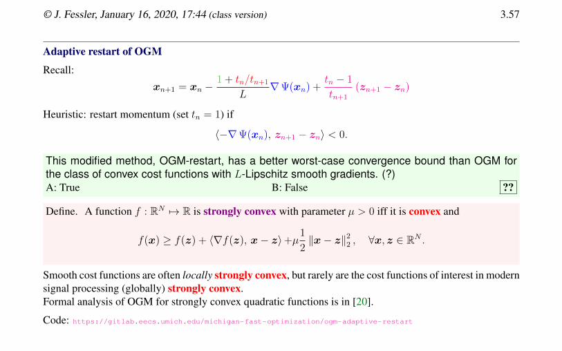
Adaptive restart of OGM
Recall:
xn+1 = xn −1 + tn/tn+1
L∇Ψ(xn) +
tn − 1
tn+1
(zn+1 − zn)
Heuristic: restart momentum (set tn = 1) if
〈−∇Ψ(xn), zn+1 − zn〉 < 0.
This modified method, OGM-restart, has a better worst-case convergence bound than OGM forthe class of convex cost functions with L-Lipschitz smooth gradients. (?)A: True B: False ??
Define. A function f : RN 7→ R is strongly convex with parameter µ > 0 iff it is convex and
f(x) ≥ f(z) + 〈∇f(z), x− z〉+µ1
2‖x− z‖2
2 , ∀x, z ∈ RN .
Smooth cost functions are often locally strongly convex, but rarely are the cost functions of interest in modernsignal processing (globally) strongly convex.Formal analysis of OGM for strongly convex quadratic functions is in [20].
Code: https://gitlab.eecs.umich.edu/michigan-fast-optimization/ogm-adaptive-restart

© J. Fessler, January 16, 2020, 17:44 (class version) 3.58
3.9 Summary
This chapter summarizes some of the most important gradient-based algorithms for solving unconstrainedoptimization problems with differentiable cost functions.
All of the methods discussed here require computing the gradient ∇Ψ(xk) each iteration, and often that isthe most expensive operation.
Some of the algorithms (PSD, PCG) also require a line search step. A line search is itself a 1D optimizationproblem that requires evaluating the cost function or its gradient multiple times, and those evaluations canadd considerable expense for general cost functions.
For cost functions of the form (3.13), where each component function fj and its gradient are easy to evaluate,one can perform a line search quite efficiently, as described on p. 3.33.
The set of cost functions of the form (3.13), where each fj has a Lipschitz continuous gradient, isa strict subset of the set of cost functions Ψ having Lipschitz continuous gradients. (?)A: True B: False ??
Recent work made a version of OGM with a line search [21].

© J. Fessler, January 16, 2020, 17:44 (class version) 3.59
Bibliography
[1] Y. Nesterov. Introductory lectures on convex optimization: A basic course. Springer, 2004 (cit. on pp. 3.8, 3.9, 3.34, 3.41, 3.44, 3.51).
[2] R. C. Fair. “On the robust estimation of econometric models”. In: Ann. Econ. Social Measurement 2 (Oct. 1974), 667–77 (cit. on p. 3.12).
[3] K. Lange. “Convergence of EM image reconstruction algorithms with Gibbs smoothing”. In: IEEE Trans. Med. Imag. 9.4 (Dec. 1990). Corrections,T-MI, 10:2(288), June 1991., 439–46 (cit. on p. 3.12).
[4] B. T. Polyak. Introduction to optimization. New York: Optimization Software Inc, 1987 (cit. on pp. 3.14, 3.35).
[5] Y. Drori and M. Teboulle. “Performance of first-order methods for smooth convex minimization: A novel approach”. In: Mathematical Programming145.1-2 (June 2014), 451–82 (cit. on pp. 3.14, 3.16, 3.39, 3.45).
[6] A. B. Taylor, J. M. Hendrickx, and Francois Glineur. “Smooth strongly convex interpolation and exact worst-case performance of first- order methods”.In: Mathematical Programming 161.1 (Jan. 2017), 307–45 (cit. on pp. 3.14, 3.44).
[7] D. Kim and J. A. Fessler. “Optimized first-order methods for smooth convex minimization”. In: Mathematical Programming 159.1 (Sept. 2016), 81–107(cit. on pp. 3.16, 3.18, 3.43, 3.44, 3.45, 3.46, 3.47, 3.51).
[8] A. Cauchy. “Methode générale pour la résolution des systems d’équations simultanées”. In: Comp. Rend. Sci. Paris 25 (1847), 536–8 (cit. on p. 3.18).
[9] A. Florescu, E. Chouzenoux, J-C. Pesquet, P. Ciuciu, and S. Ciochina. “A majorize-minimize memory gradient method for complex-valued inverseproblems”. In: Signal Processing 103 (Oct. 2014), 285–95 (cit. on pp. 3.25, 3.26).
[10] J. A. Fessler. Image reconstruction: Algorithms and analysis. Book in preparation. ., 2006 (cit. on pp. 3.31, 3.38, 3.39).
[11] J. Barzilai and J. Borwein. “Two-point step size gradient methods”. In: IMA J. Numerical Analysis 8.1 (1988), 141–8 (cit. on p. 3.42).
[12] Y. Nesterov. “A method for unconstrained convex minimization problem with the rate of convergence O(1/k2)”. In: Dokl. Akad. Nauk. USSR 269.3(1983), 543–7 (cit. on p. 3.43).
[13] Y. Nesterov. “Smooth minimization of non-smooth functions”. In: Mathematical Programming 103.1 (May 2005), 127–52 (cit. on p. 3.43).
[14] O. Güler. “New proximal point algorithms for convex minimization”. In: SIAM J. Optim. 2.4 (1992), 649–64 (cit. on p. 3.47).
[15] D. Kim and J. A. Fessler. “On the convergence analysis of the optimized gradient methods”. In: J. Optim. Theory Appl. 172.1 (Jan. 2017), 187–205(cit. on pp. 3.47, 3.48, 3.51).

© J. Fessler, January 16, 2020, 17:44 (class version) 3.60
[16] Y. Drori. “The exact information-based complexity of smooth convex minimization”. In: J. Complexity 39 (Apr. 2017), 1–16 (cit. on p. 3.50).
[17] A. B. Taylor, J. M. Hendrickx, and Francois Glineur. “Exact worst-case performance of first-order methods for composite convex optimization”. In:SIAM J. Optim. 27.3 (Jan. 2017), 1283–313 (cit. on p. 3.53).
[18] D. Böhning and B. G. Lindsay. “Monotonicity of quadratic approximation algorithms”. In: Ann. Inst. Stat. Math. 40.4 (Dec. 1988), 641–63.
[19] B. O’Donoghue and E. Candes. “Adaptive restart for accelerated gradient schemes”. In: Found. Comp. Math. 15.3 (June 2015), 715–32 (cit. on p. 3.56).
[20] D. Kim and J. A. Fessler. “Adaptive restart of the optimized gradient method for convex optimization”. In: J. Optim. Theory Appl. 178.1 (July 2018),240–63 (cit. on pp. 3.56, 3.57).
[21] Y. Drori and A. B. Taylor. Efficient first-order methods for convex minimization: a constructive approach. 2018 (cit. on p. 3.58).