Embed Size (px)
Citation preview
Chapter 3
Frailty Models Based on the
Gompertz Baseline Distribution
3.1 Introduction
Mostly Weibull distribution is considered for baseline hazard. It is well known that the Weibull
model is not suitable for modeling survival data in all situations. Gompertz distribution is one of
the most important growth models. It has many applications in, for example, medical, biological
and actuarial studies. The Gompertz distribution plays an important role in modeling human
mortality and fitting actuarial tables. It has been used as a growth model and also used to fit
the tumor growth.
This Chapter consider shared frailty models with Gompertz baseline distribution. The mate-
rial of this Chapter i.e. Shared gamma frailty model with Gompertz baseline has been accepted
by the journal Statistics and Probability Letters, 82, 1310-17, (2012) and the remaining content
of this Chapter i.e. Shared inverse Gaussian frailty model with Gompertz baseline has been
submitted for publication in the well-known international journal.
57
Gompertz Baseline Distribution 58
3.2 Gompertz Baseline Distribution
Gompertz model, used most frequently by medical researchers and biologists in modeling the
mortality ratio data, was formulated by Gompertz (1825). Gompertz distribution is a growth
model and has been used in relation with tumor development. Ahuja and Nash (1979) showed
that Gompertz distribution, with a simple conversion, related to some distributions in the Pear-
son distributions family. According to Jaheen (2003), Garg et al. (1970) obtained the maximum
likelihood estimations of the Gompertz distribution parameters. Osman (1987), used a Gompertz
distribution with two parameters, worked on the features of the distribution and offered that it
should be used in modeling the lifespan data analyzing the survival ratio in heterogenic masses.
It has been widely used, especially in actuarial and biological applications and in demography.
A continuous random variable T is said to follow a Gompertz distribution with parameters
λ > 0 and γ > 0 (T ∼ Gompertz(λ, γ)), if the baseline hazard function corresponds to
h0(t) =
λ exp(γ t) ; t > 0, λ > 0, γ ∈ R
0 ; otherwise.(3.1)
and the cumulative hazard function is
H0(t) =
λγ−1(exp(γ t)− 1) ; t > 0, λ > 0, γ ∈ R
0 ; otherwise.(3.2)
where λ and γ are scale and shape parameters, respectively. For γ = 0 the baseline hazard (3.1)
reduces to the exponential hazard.
The corresponding survival function and probability density function of Gompertz distribu-
tion are
S0(t) =
exp[−λγ−1(exp(γt)− 1)] ; t > 0, λ > 0, γ ∈ R
0 ; otherwise.(3.3)
and
f0(t) =
λ exp(γ t) exp[−λγ−1(exp(γt)− 1)] ; t > 0, λ > 0, γ ∈ R
0 ; otherwise.(3.4)
We note that for γ > 0, S0(t) goes to zero for t→∞. With γ < 0, S0(t) goes to 0 < exp(λγ−1) <
1 for t → ∞. Therefore the event never occurs for a proportion exp(λγ−1) of the population.
We therefore consider the case γ > 0.
Gompertz Baseline Distribution 59
In this Chapter, the two-parameter Gompertz distribution is considered. Let us assume that
the independent random variables T1 and T2 have Gompertz distribution with parameters λ1, γ1
and λ2, γ2, respectively. In short we say Gomp(λj , γj), (j = 1, 2).
Here, T1 and T2 are independent, thus, H(ti1, ti2) = H1(ti1) + H2(ti2), where Hj(tij) is the
integrated hazard of Tij , (i = 1, 2, ..., n; j = 1, 2).
Under this independency assumption, using equation (1.1), the resulting regression model
H(tij |Ui, Xi) = uiλjγ−1
j (exp(γj tij)− 1) exp(x′iβ), (i = 1, .....n; j = 1, 2) (3.5)
is indeed an extended cumulative proportional hazards model conditional on frailty and fixed
factors. The conditional survival function of the jth individual in the ith cluster is given by
S(tij |Ui, Xi) = exp[−uiλjγ−1
j exp(x′iβ)(exp(γj tij)− 1)], tij ≥ 0, λj > 0, γj > 0 (3.6)
Here value of Ui is common to two components in a group. When there is no variability in the
distribution of Ui, that is, when Ui has a degenerate distribution then there is no dependency.
When the distribution is not degenerate, the dependence is positive. The value of Ui can be
considered as generated from unknown values of some explanatory variables. Conditional on
Ui = ui, the bivariate survival function is
S(ti1, ti2|Ui, Xi) = S(ti1|Ui, Xi)S(ti2|Ui, Xi)
= exp[−ui exp(x′iβ){λ1γ−11 (exp(γ1ti1)− 1) + λ2γ
−12 (exp(γ2ti2)− 1)}] (3.7)
where Ui (i = 1, 2, · · · , n) follows gamma distribution and inverse Gaussian distribution given
in (1.7) and (1.18), respectively.
3.2.1 Proposed Models
Substituting cumulative hazard function for Gompertz distribution in equations (1.9) and (1.20),
we get the unconditional bivariate survival functions based on gamma frailty and inverse Gaus-
sian frailty as,
Sθ(ti1, ti2|Xi) = [1 + θ exp(x′iβ){λ1γ−11 (exp(γ1ti1)− 1) + λ2γ
−12 (exp(γ2ti2)− 1)}]−1/θ (3.8)
Gompertz Baseline Distribution 60
and
Sθ(ti1, ti2|Xi) = exp[
1− (1 + 2θ exp(x′iβ){λ1γ−11 (exp(γ1ti1)− 1) + λ2γ
−12 (exp(γ2ti2)− 1)})1/2
θ
](3.9)
Here onwards we call equations (3.8) and (3.9) as Model-I and Model-II, respectively. Thus,
Model-I is the shared gamma frailty model under Gompertz baseline hazard and Model-II is the
shared inverse Gaussian frailty model under the same Gompertz baseline hazard.
Once we have unconditional survival function of bivariate random variable (Ti1, Ti2) we can
obtain likelihood function and estimate the parameters of the model. Here onwards in this
Chapter we represent Sθ(ti1, ti2|Xi) as Sθ(ti1, ti2).
3.3 Fitting of Models
Inferential procedures for frailty models have almost exclusively focused on likelihood based
approaches (Liang et al., 1995). The likelihood function in (2.7) for the random censorship
model can be used for the estimation procedure. To estimate the parameters of the model firstly
we must have to obtain likelihood function given by (2.7) for which we need to obtain the
functions, fi1, fi2, fi3, and Fi. Differentiating survival function for each of the model given in
equations (3.8) and (3.9) for obtaining these functions.
For Model-I, we have
fi1 = (1 + θ)λ1λ2 exp(2x′iβ) exp(γ1ti1 + γ2ti2)S(1+2θ)θ (ti1, ti2)
fi2 = λ1 exp(x′iβ) exp(γ1ti1)S(1+θ)θ (ti1, wi)
fi3 = λ2 exp(x′iβ) exp(γ2ti2)S(1+θ)θ (wi, ti2)
Fi = Sθ(wi, wi)
where Sθ(., .) is given by equation (3.8).
Gompertz Baseline Distribution 61
For Model-II, we have
fi1 =λ1λ2 exp(γ1ti1 + γ2ti2)Sθ(ti1, ti2)φ2(ti1, ti2)
[φ1(ti1, ti2)]32
exp(2x′iβ)
fi2 =λ1 exp(γ1ti1)Sθ(ti1, wi)
[φ1(ti1, wi)]12
exp(x′iβ)
fi3 =λ2 exp(γ2ti2)Sθ(wi, ti2)
[φ1(wi, ti2)]12
exp(x′iβ)
Fi = Sθ(wi, wi)
where φ1(ai, bi) = 1 + 2θ{λ1γ−11 (exp(γ1ai − 1)) + λ2γ
−12 (exp(γ2bi − 1))} exp(x′iβ); φ2(ai, bi) =
θ + [φ1(ai, bi)]12 and Sθ(., .) is given by equation (3.9).
Now we apply MCMC procedure discussed in Section (2.5) to estimate the parameters of
the models. Firstly, we consider a simulation study to evaluate the performance of the Bayesian
estimation procedure and then we apply the procedure to litters of rat data.
3.4 Simulation Study
To evaluate the performance of the Bayesian estimation procedure we carried out a simulation
study. For the simulation purpose we have considered only one covariate X = X1 which we
assume to follow binomial distribution for Model-I and normal distribution for Model-II. With
one covariate, the shared gamma frailty model and the shared inverse Gaussian frailty model
given in equation (3.8) and (3.9), respectively, has six parameters. The frailty variable U is
assumed to have gamma distribution and inverse Gaussian distribution with variance θ. Lifetimes
(Ti1, Ti2) for ith pair are conditionally independent for given frailty Ui = ui. We assume that
Tij (i = 1, . . . , n; j = 1, 2) follows the Gompertz baseline distribution. As the Bayesian methods
are time consuming, we generate only fifty, seventy-five and one hundred pairs of lifetimes using
inverse transform technique.
According to the assumption, for given frailty U , lifetimes of individuals are independent.
So, the conditional survival function for an individual for given frailty U = u and a covariate X
at time t > 0 is,
S(t | U,X) = exp[−uH0(t) exp(x′iβ)] (3.10)
Gompertz Baseline Distribution 62
Equating S(t | U,X) to a random number say r (0 < r < 1) over t > 0, using (3.6), we get,
t = γ−1ln
[1 +
γA
λ
](3.11)
where A = − ln(r)u exp(xβ) . Equations (3.11) is a generator to generate lifetimes for model (3.8) and
(3.9). We have generated different random samples of size n = 50, 75 and 100 for lifetimes Ti1
and Ti2 using (3.11) and for frailty from gamma and inverse Gaussian density functions f(u)
given in (1.7) and (1.18). To generate frailty values from gamma distribution we have used direct
commands in R package but for generating frailty values from inverse Gaussian distribution we
have used different packages like ‘SuppDists’, ‘statmod’ etc. in R.
Here we have generated different random samples of size n = 50, 75 and 100 for lifetimes Ti1
and Ti2 using (3.11). But we are giving procedure for sample generation of only one sample size,
say, n = 50. Samples are generated using following procedure for Model-I and Model-II:
1. Generate a random sample of size n = 50 from gamma and inverse Gaussian distributions
having density as given in equation (1.7) and (1.18), with θ = 3.6 as shared frailties (ui)
for ith (i = 1, 2, . . . , 50) cluster.
2. Generate 50 covariate values for X from binomial distribution for Model-I and from normal
distribution for Model-II.
3. Compute exp(Xiβ) with regression coefficient β = 2 and β = 0.7 for Model-I and Model-II,
respectively.
4. Generate 50 pairs of lifetimes (ti1, ti2) for given covariate (xi) using following generators,
ti1 = γ−11 ln
[1 +
γ1Ai1λ1
](3.12)
ti2 = γ−12 ln
[1 +
γ2Ai2λ2
](3.13)
for shared frailty models Model-I and Model-II, where Ai1 = − ln(ri1)ui exp(xiβ) and Ai2 =
− ln(ri2)ui exp(xiβ) ; r1 and r2 are random variables having U(0, 1) distribution and γ1, λ1 are
respectively shape and scale parameters of baseline distribution of first survival time and
γ2, λ2 are that of second survival time.
Gompertz Baseline Distribution 63
5. Generate censoring time wi from exponential distribution with failure rate 0.9 for Model-I
and 1.5 for Model-II.
6. Observe jth individual survival time t∗ij = min(tij , wi) and censoring indicator δij for ith
cluster (i = 1, 2, . . . , 50 and j = 1, 2), where
δij =
1, ; tij ≤ wi
0, ; tij > wi
Thus we have data consists of 50 pairs of survival times (t∗i1, t∗i2) and censoring indicators
δij .
Prior distributions that we have assumed for the parameters of Model-I are respec-
tively, G(0.0001, 0.0001) for baseline parameters λ1, γ1 and γ2 and G(0.01, 0.01) for λ2;
G(0.0001, 0.0001) for frailty parameter θ and N(0, 1000) for regression parameter β. Also,
prior distributions that we have assumed for the parameters of Model-II are respectively,
G(0.0001, 0.0001) for baseline parameters λ1, λ2, γ1 and γ2; G(0.0001, 0.0001) for frailty pa-
rameter θ and N(0, 1000) for regression parameter β. Here G(a, b) is gamma distribution with
shape parameter a and scale parameter b and N(µ, σ2) represents normal distribution with mean
µ and variance σ2.
We run two parallel chains for the proposed model with the different starting points using
Metropolis-Hastings algorithm within Gibbs sampler based on normal transition kernels. We
have iterated both the chains for 95,000 times using gamma prior. For both the chains the
results were somewhat similar so we present here the analysis for only one chain (i.e. chain I)
and for only one sample size for the resulting shared frailty models.
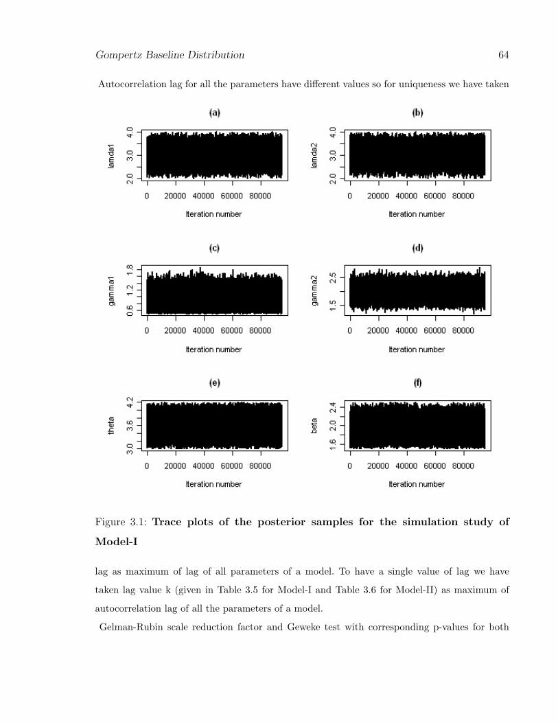
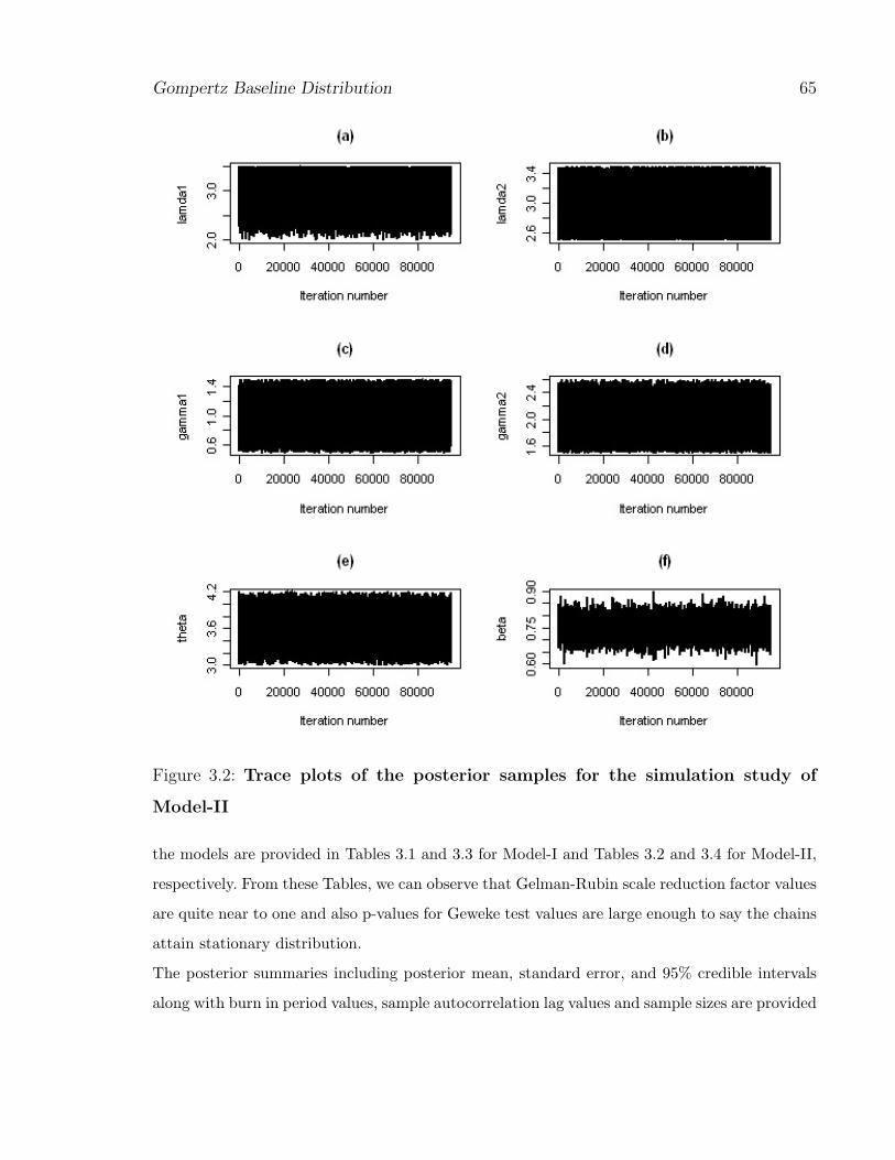
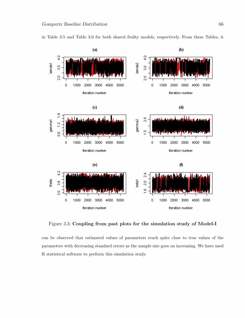
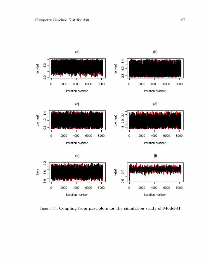
Trace plots and coupling from past plots are presented in Figures 3.1 and 3.3 for Model-I and
Figures 3.2 and 3.4 for Model-II with gamma prior assumption. These plots for other sample sizes
also have same pattern. So, we have not shown any graphs for other sample sizes, only for n = 75
with gamma prior has been shown to get the idea about these graphs. Trace plots are having
zigzag pattern which says that parameters are moving freely and appropriate for both models.
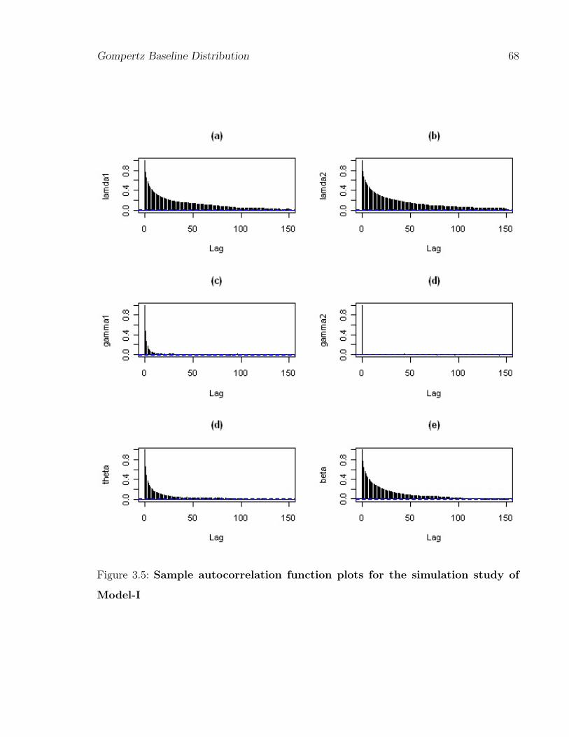
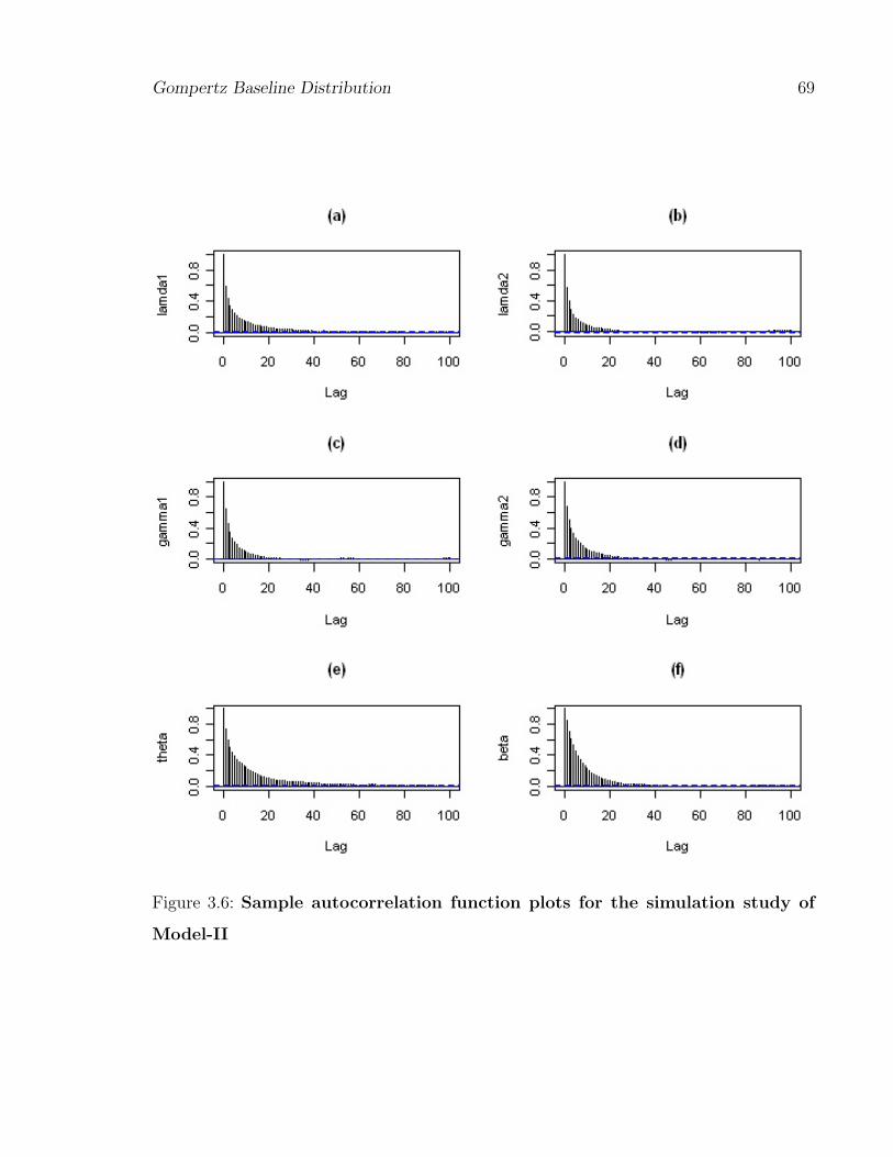
Sample autocorrelation plots are presented in Figures 3.5 and 3.6 for both models. Generated
chains have slightly higher autocorrelation lag which is decided by using sample autocorrelation
function plot.
Gompertz Baseline Distribution 64
Autocorrelation lag for all the parameters have different values so for uniqueness we have taken
Figure 3.1: Trace plots of the posterior samples for the simulation study of
Model-I
lag as maximum of lag of all parameters of a model. To have a single value of lag we have
taken lag value k (given in Table 3.5 for Model-I and Table 3.6 for Model-II) as maximum of
autocorrelation lag of all the parameters of a model.
Gelman-Rubin scale reduction factor and Geweke test with corresponding p-values for both
Gompertz Baseline Distribution 65
Figure 3.2: Trace plots of the posterior samples for the simulation study of
Model-II
the models are provided in Tables 3.1 and 3.3 for Model-I and Tables 3.2 and 3.4 for Model-II,
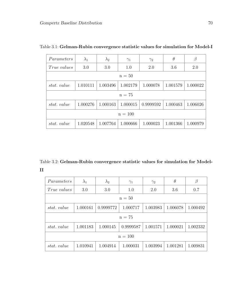
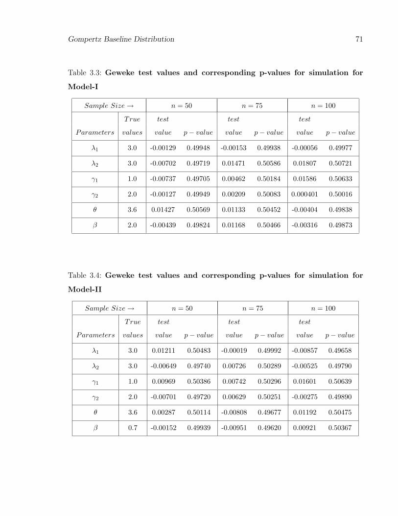
respectively. From these Tables, we can observe that Gelman-Rubin scale reduction factor values
are quite near to one and also p-values for Geweke test values are large enough to say the chains
attain stationary distribution.
The posterior summaries including posterior mean, standard error, and 95% credible intervals
along with burn in period values, sample autocorrelation lag values and sample sizes are provided
Gompertz Baseline Distribution 66
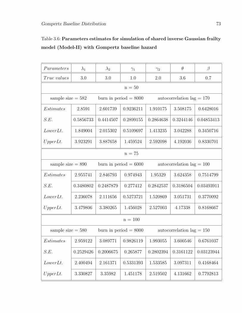
in Table 3.5 and Table 3.6 for both shared frailty models, respectively. From these Tables, it
Figure 3.3: Coupling from past plots for the simulation study of Model-I
can be observed that estimated values of parameters reach quite close to true values of the
parameters with decreasing standard errors as the sample size goes on increasing. We have used
R statistical software to perform this simulation study.
Gompertz Baseline Distribution 67
Figure 3.4: Coupling from past plots for the simulation study of Model-II
Gompertz Baseline Distribution 68
Figure 3.5: Sample autocorrelation function plots for the simulation study of
Model-I
Gompertz Baseline Distribution 69
Figure 3.6: Sample autocorrelation function plots for the simulation study of
Model-II
Gompertz Baseline Distribution 70
Table 3.1: Gelman-Rubin convergence statistic values for simulation for Model-I
Parameters λ1 λ2 γ1 γ2 θ β
True values 3.0 3.0 1.0 2.0 3.6 2.0
n = 50
stat. value 1.010111 1.003496 1.002179 1.000078 1.001579 1.000022
n = 75
stat. value 1.000276 1.000163 1.000015 0.9999592 1.000463 1.006026
n = 100
stat. value 1.020548 1.007764 1.000666 1.000023 1.001366 1.000979
Table 3.2: Gelman-Rubin convergence statistic values for simulation for Model-
II
Parameters λ1 λ2 γ1 γ2 θ β
True values 3.0 3.0 1.0 2.0 3.6 0.7
n = 50
stat. value 1.000161 0.9999772 1.000717 1.003983 1.006078 1.000492
n = 75
stat. value 1.001183 1.000145 0.9999587 1.001571 1.000021 1.002332
n = 100
stat. value 1.010941 1.004914 1.000031 1.003994 1.001281 1.009831
Gompertz Baseline Distribution 71
Table 3.3: Geweke test values and corresponding p-values for simulation for
Model-I
Sample Size→ n = 50 n = 75 n = 100
True test test test
Parameters values value p− value value p− value value p− value
λ1 3.0 -0.00129 0.49948 -0.00153 0.49938 -0.00056 0.49977
λ2 3.0 -0.00702 0.49719 0.01471 0.50586 0.01807 0.50721
γ1 1.0 -0.00737 0.49705 0.00462 0.50184 0.01586 0.50633
γ2 2.0 -0.00127 0.49949 0.00209 0.50083 0.000401 0.50016
θ 3.6 0.01427 0.50569 0.01133 0.50452 -0.00404 0.49838
β 2.0 -0.00439 0.49824 0.01168 0.50466 -0.00316 0.49873
Table 3.4: Geweke test values and corresponding p-values for simulation for
Model-II
Sample Size→ n = 50 n = 75 n = 100
True test test test
Parameters values value p− value value p− value value p− value
λ1 3.0 0.01211 0.50483 -0.00019 0.49992 -0.00857 0.49658
λ2 3.0 -0.00649 0.49740 0.00726 0.50289 -0.00525 0.49790
γ1 1.0 0.00969 0.50386 0.00742 0.50296 0.01601 0.50639
γ2 2.0 -0.00701 0.49720 0.00629 0.50251 -0.00275 0.49890
θ 3.6 0.00287 0.50114 -0.00808 0.49677 0.01192 0.50475
β 0.7 -0.00152 0.49939 -0.00951 0.49620 0.00921 0.50367

Gompertz Baseline Distribution 72
Table 3.5: Parameters estimates for simulation of shared gamma frailty model
(Model-I) with Gompertz baseline hazard
Parameters λ1 λ2 γ1 γ2 θ β
True values 3.0 3.0 1.0 2.0 3.6 2.0
n = 50
sample size = 870 burn in period = 8000 autocorrelation lag = 100
Estimates 3.339832 3.58423 0.8029933 1.898675 3.728842 1.784984
S.E. 0.5166535 0.5047603 0.2513277 0.2350126 0.3168721 0.2564108
LowerLt. 2.17248 2.030812 0.51023 1.603307 3.039895 1.519136
UpperLt. 3.935928 3.862703 1.464501 2.375263 4.159701 2.412618
n = 75
sample size = 600 burn in period = 5000 autocorrelation lag = 150
Estimates 3.275938 3.352028 0.9781125 1.990647 3.670445 1.807583
S.E. 0.4715845 0.4150472 0.2474298 0.1986308 0.2753138 0.2123236
LowerLt. 2.235856 2.462795 0.550843 1.609894 3.114257 1.521822
UpperLt. 3.927783 3.967307 1.498642 2.360427 4.147788 2.286009
n = 100
sample size = 425 burn in period = 10000 autocorrelation lag = 200
Estimates 2.818765 2.805313 1.019907 1.997276 3.601107 1.829282
S.E. 0.4173838 0.3207179 0.2032705 0.1980163 0.2688608 0.2091362
LowerLt. 2.283129 2.876453 0.5884597 1.621737 3.180849 1.516968
UpperLt. 3.783039 3.992017 1.409367 2.37215 4.156142 2.259177
Gompertz Baseline Distribution 73
Table 3.6: Parameters estimates for simulation of shared inverse Gaussian frailty
model (Model-II) with Gompertz baseline hazard
Parameters λ1 λ2 γ1 γ2 θ β
True values 3.0 3.0 1.0 2.0 3.6 0.7
n = 50
sample size = 582 burn in period = 8000 autocorrelation lag = 170
Estimates 2.8591 2.601739 0.9236211 1.910175 3.508175 0.6428016
S.E. 0.5856733 0.4414507 0.2899155 0.2864638 0.3244146 0.04853413
LowerLt. 1.849004 2.015302 0.5109697 1.413235 3.042288 0.3450716
UpperLt. 3.923291 3.887658 1.459524 2.592098 4.192036 0.8330701
n = 75
sample size = 890 burn in period = 6000 autocorrelation lag = 100
Estimates 2.955741 2.846793 0.974943 1.95329 3.624358 0.7514799
S.E. 0.3480802 0.2487879 0.277412 0.2842537 0.3186504 0.03493911
LowerLt. 2.236078 2.111656 0.5273721 1.520869 3.051731 0.3770092
UpperLt. 3.479806 3.380265 1.456028 2.527003 4.17338 0.8168667
n = 100
sample size = 580 burn in period = 8000 autocorrelation lag = 150
Estimates 2.959122 3.089771 0.9826119 1.993055 3.600546 0.6761037
S.E. 0.2529426 0.2006675 0.265877 0.2802394 0.3161122 0.03123944
LowerLt. 2.400494 2.161371 0.5331393 1.533585 3.097311 0.4168464
UpperLt. 3.330827 3.35982 1.451178 2.519502 4.131662 0.7792813
Gompertz Baseline Distribution 74
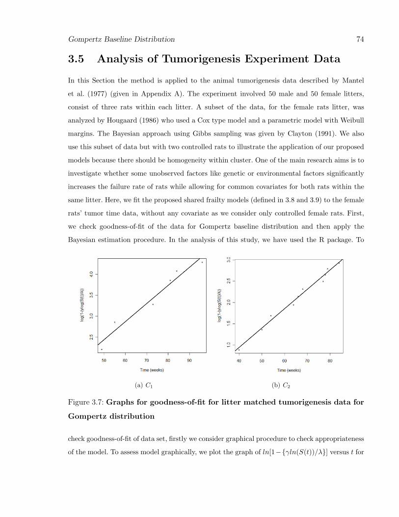
3.5 Analysis of Tumorigenesis Experiment Data
In this Section the method is applied to the animal tumorigenesis data described by Mantel
et al. (1977) (given in Appendix A). The experiment involved 50 male and 50 female litters,
consist of three rats within each litter. A subset of the data, for the female rats litter, was
analyzed by Hougaard (1986) who used a Cox type model and a parametric model with Weibull
margins. The Bayesian approach using Gibbs sampling was given by Clayton (1991). We also
use this subset of data but with two controlled rats to illustrate the application of our proposed
models because there should be homogeneity within cluster. One of the main research aims is to
investigate whether some unobserved factors like genetic or environmental factors significantly
increases the failure rate of rats while allowing for common covariates for both rats within the
same litter. Here, we fit the proposed shared frailty models (defined in 3.8 and 3.9) to the female
rats’ tumor time data, without any covariate as we consider only controlled female rats. First,
we check goodness-of-fit of the data for Gompertz baseline distribution and then apply the
Bayesian estimation procedure. In the analysis of this study, we have used the R package. To
(a) C1 (b) C2
Figure 3.7: Graphs for goodness-of-fit for litter matched tumorigenesis data for
Gompertz distribution
check goodness-of-fit of data set, firstly we consider graphical procedure to check appropriateness
of the model. To assess model graphically, we plot the graph of ln[1−{γln(S(t))/λ}] versus t for
Gompertz Baseline Distribution 75
proposed model. If the resulted plot is roughly a straight line then we can say that the underline
baseline model is appropriate. The graph of ln[1−{γln(S(t))/λ}] versus t for Gompertz baseline
distribution for both controlled rats C1 and C2, using R-program, are shown in the Figures 3.7(a)
and 3.7(b), respectively. From the Figures, we can observe that many of the points are nearly
on the straight line.
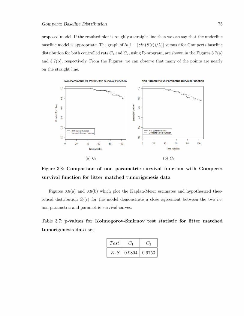
(a) C1 (b) C2
Figure 3.8: Comparison of non parametric survival function with Gompertz
survival function for litter matched tumorigenesis data
Figures 3.8(a) and 3.8(b) which plot the Kaplan-Meier estimates and hypothesized theo-
retical distribution S0(t) for the model demonstrate a close agreement between the two i.e.
non-parametric and parametric survival curves.
Table 3.7: p-values for Kolmogorov-Smirnov test statistic for litter matched
tumorigenesis data set
Test C1 C2
K-S 0.9804 0.9753
Gompertz Baseline Distribution 76
We have considered a statistical test also viz. Kolmogorov-Smirnov (K-S) test for testing
composite goodness-of-fit hypotheses to the Gompertz baseline distribution for models (3.8)
and (3.9). Test procedure is developed for testing goodness-of-fit with data subjected to random
right censoring. Here, we assume that survival times of rats are conditionally independent so
we apply K-S test to the survival times of both rats separately. The p-values of K-S test for
baseline distribution are presented in Table 3.7 which are very large approximately close to 1.
Thus, from different goodness-of-fit graphs (see Figures 3.7(a) and 3.7(b)) and p-values of K-S
test (see Table 3.7) we can say that there is no statistical evidence to reject the hypothesis that
data are from Gompertz distribution.
In the analysis, we have used the R program. Given the model assumptions, this program
performs the Gibbs sampler by simulating from the full conditional distributions. We run two
parallel chains for both shared frailty models using two sets of prior distributions with the
different starting points using Metropolis-Hastings algorithm within Gibbs sampler based on
normal transition kernels. In our study of this data, the prior distribution we use for frailty
parameter θ is gamma distribution with mean one and large variance, say Γ(φ, φ), with a small
choice of φ. Since, we do not have any prior information about baseline parameters, λ1, γ1, λ2,
and γ2, therefore, prior distributions of these parameters are assumed to be flat. We consider
two different sets of prior distributions for baseline parameters, one is Γ(a, b) and another is
U(c, d). All the hyper-parameters φ, a, b, c, and d are known. Here Γ(a, b) is gamma distribution
with shape parameter a and scale parameter b and U(c, d) represents uniform distribution over
the interval c to d. We set hyper-parameters as
• for Model-I
φ = 0.00001, a = 1; b = 0.0001, c = 0 and d = 100.
• for Model-II
φ = 0.00001; a = 1, b = 0.0001 for λ1, λ2, γ1, and γ2; and c = 0, d = 100 for λ1, λ2, γ2,
and c = 0, d = 60 for γ1.
We implemented 95,000 iterations of the algorithm. To diminish the effect of the starting
distribution, we generally discard the early iterations of each sequence and focus attention on
the remaining.
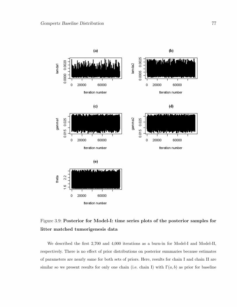
Gompertz Baseline Distribution 77
Figure 3.9: Posterior for Model-I: time series plots of the posterior samples for
litter matched tumorigenesis data
We described the first 2,700 and 4,000 iterations as a burn-in for Model-I and Model-II,
respectively. There is no effect of prior distributions on posterior summaries because estimates
of parameters are nearly same for both sets of priors. Here, results for chain I and chain II are
similar so we present results for only one chain (i.e. chain I) with Γ(a, b) as prior for baseline
Gompertz Baseline Distribution 78
parameters.
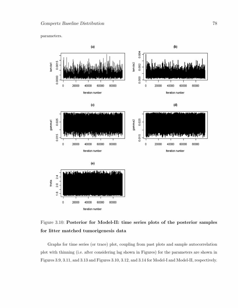
Figure 3.10: Posterior for Model-II: time series plots of the posterior samples
for litter matched tumorigenesis data
Graphs for time series (or trace) plot, coupling from past plots and sample autocorrelation
plot with thinning (i.e. after considering lag shown in Figures) for the parameters are shown in
Figures 3.9, 3.11, and 3.13 and Figures 3.10, 3.12, and 3.14 for Model-I and Model-II, respectively.
Gompertz Baseline Distribution 79
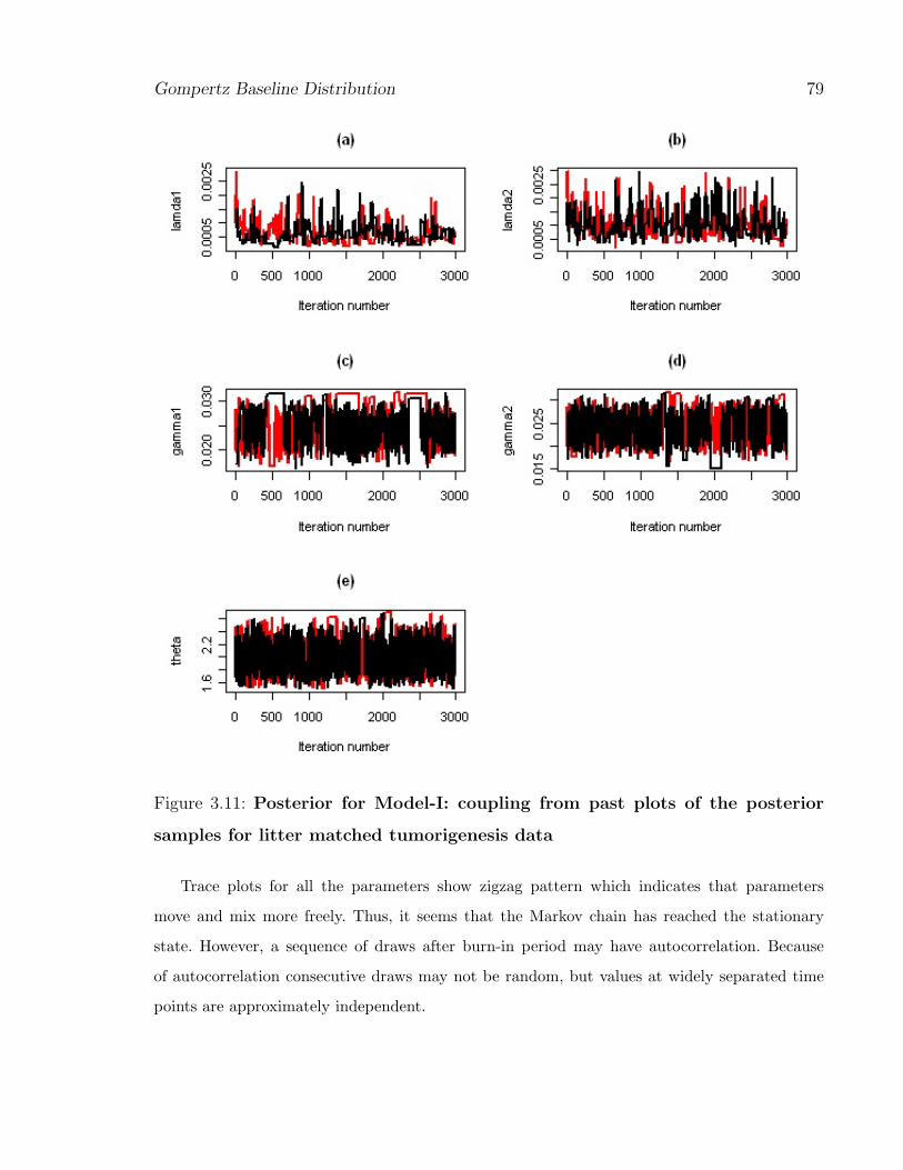
Figure 3.11: Posterior for Model-I: coupling from past plots of the posterior
samples for litter matched tumorigenesis data
Trace plots for all the parameters show zigzag pattern which indicates that parameters
move and mix more freely. Thus, it seems that the Markov chain has reached the stationary
state. However, a sequence of draws after burn-in period may have autocorrelation. Because
of autocorrelation consecutive draws may not be random, but values at widely separated time
points are approximately independent.
Gompertz Baseline Distribution 80
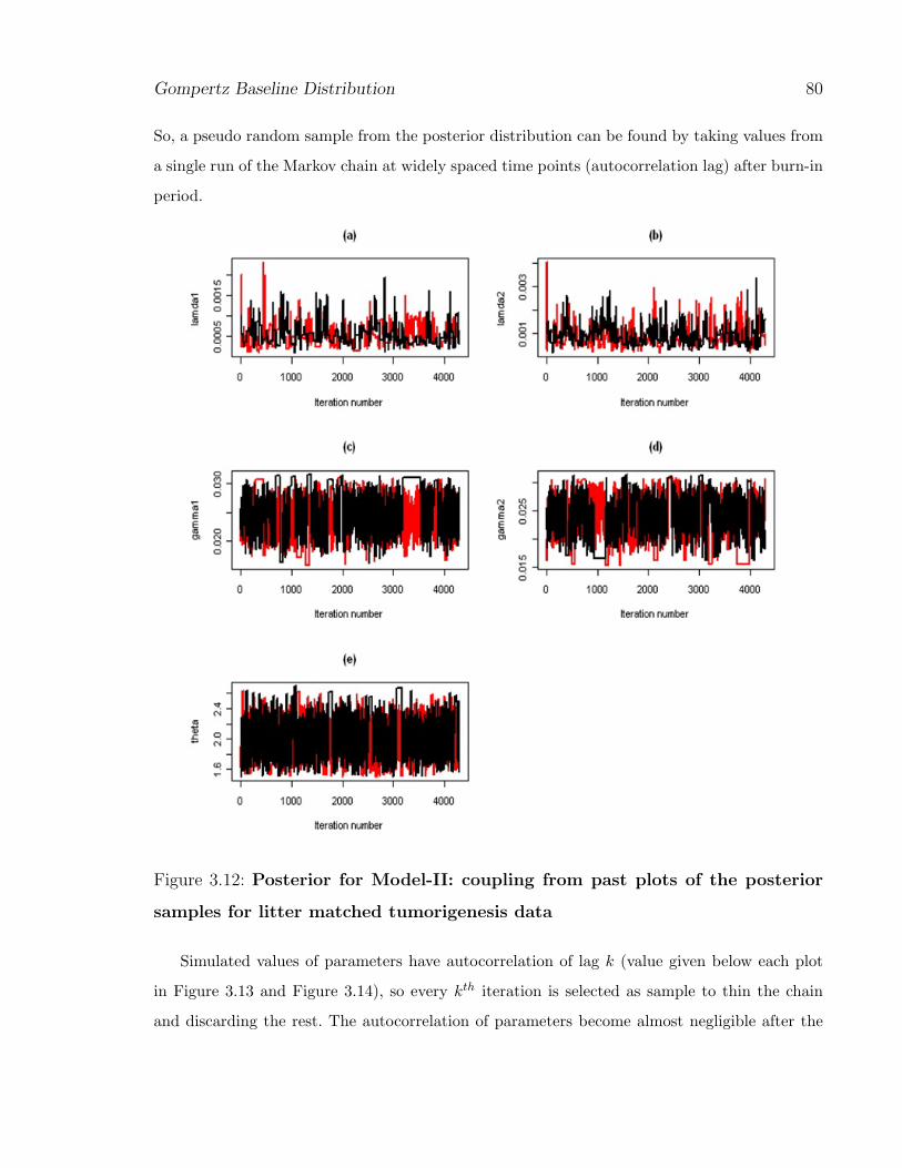
So, a pseudo random sample from the posterior distribution can be found by taking values from
a single run of the Markov chain at widely spaced time points (autocorrelation lag) after burn-in
period.
Figure 3.12: Posterior for Model-II: coupling from past plots of the posterior
samples for litter matched tumorigenesis data
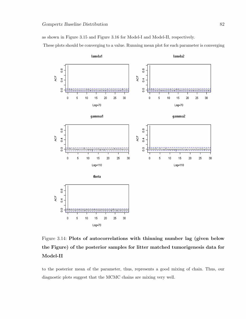
Simulated values of parameters have autocorrelation of lag k (value given below each plot
in Figure 3.13 and Figure 3.14), so every kth iteration is selected as sample to thin the chain
and discarding the rest. The autocorrelation of parameters become almost negligible after the
Gompertz Baseline Distribution 81
defined lag, given in Figures.
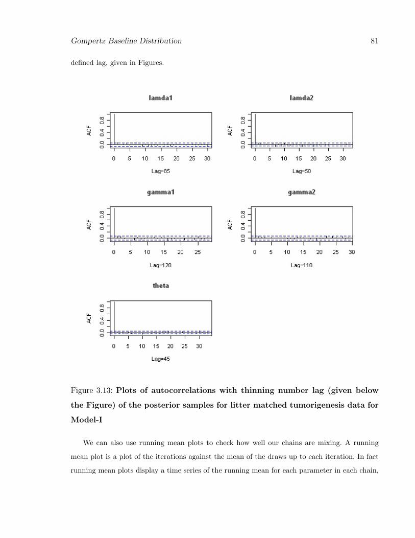
Figure 3.13: Plots of autocorrelations with thinning number lag (given below
the Figure) of the posterior samples for litter matched tumorigenesis data for
Model-I
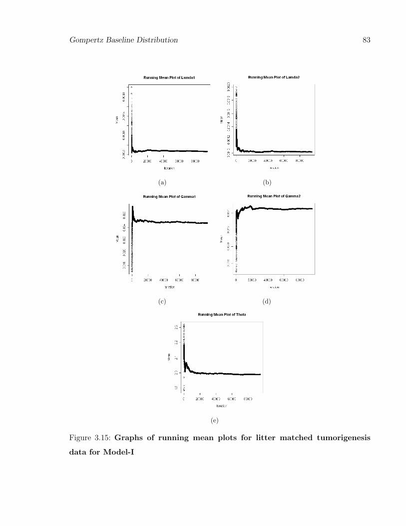
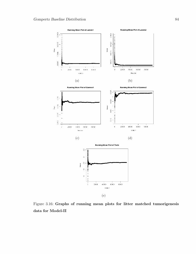
We can also use running mean plots to check how well our chains are mixing. A running
mean plot is a plot of the iterations against the mean of the draws up to each iteration. In fact
running mean plots display a time series of the running mean for each parameter in each chain,
Gompertz Baseline Distribution 82
as shown in Figure 3.15 and Figure 3.16 for Model-I and Model-II, respectively.
These plots should be converging to a value. Running mean plot for each parameter is converging
Figure 3.14: Plots of autocorrelations with thinning number lag (given below
the Figure) of the posterior samples for litter matched tumorigenesis data for
Model-II
to the posterior mean of the parameter, thus, represents a good mixing of chain. Thus, our
diagnostic plots suggest that the MCMC chains are mixing very well.
Gompertz Baseline Distribution 83
(a) (b)
(c) (d)
(e)
Figure 3.15: Graphs of running mean plots for litter matched tumorigenesis
data for Model-I
Gompertz Baseline Distribution 84
(a) (b)
(c) (d)
(e)
Figure 3.16: Graphs of running mean plots for litter matched tumorigenesis
data for Model-II
Gompertz Baseline Distribution 85
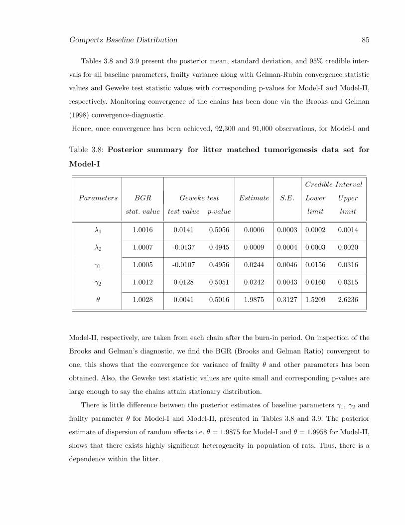
Tables 3.8 and 3.9 present the posterior mean, standard deviation, and 95% credible inter-
vals for all baseline parameters, frailty variance along with Gelman-Rubin convergence statistic
values and Geweke test statistic values with corresponding p-values for Model-I and Model-II,
respectively. Monitoring convergence of the chains has been done via the Brooks and Gelman
(1998) convergence-diagnostic.
Hence, once convergence has been achieved, 92,300 and 91,000 observations, for Model-I and
Table 3.8: Posterior summary for litter matched tumorigenesis data set for
Model-I
Credible Interval
Parameters BGR Geweke test Estimate S.E. Lower Upper
stat. value test value p-value limit limit
λ1 1.0016 0.0141 0.5056 0.0006 0.0003 0.0002 0.0014
λ2 1.0007 -0.0137 0.4945 0.0009 0.0004 0.0003 0.0020
γ1 1.0005 -0.0107 0.4956 0.0244 0.0046 0.0156 0.0316
γ2 1.0012 0.0128 0.5051 0.0242 0.0043 0.0160 0.0315
θ 1.0028 0.0041 0.5016 1.9875 0.3127 1.5209 2.6236
Model-II, respectively, are taken from each chain after the burn-in period. On inspection of the
Brooks and Gelman’s diagnostic, we find the BGR (Brooks and Gelman Ratio) convergent to
one, this shows that the convergence for variance of frailty θ and other parameters has been
obtained. Also, the Geweke test statistic values are quite small and corresponding p-values are
large enough to say the chains attain stationary distribution.
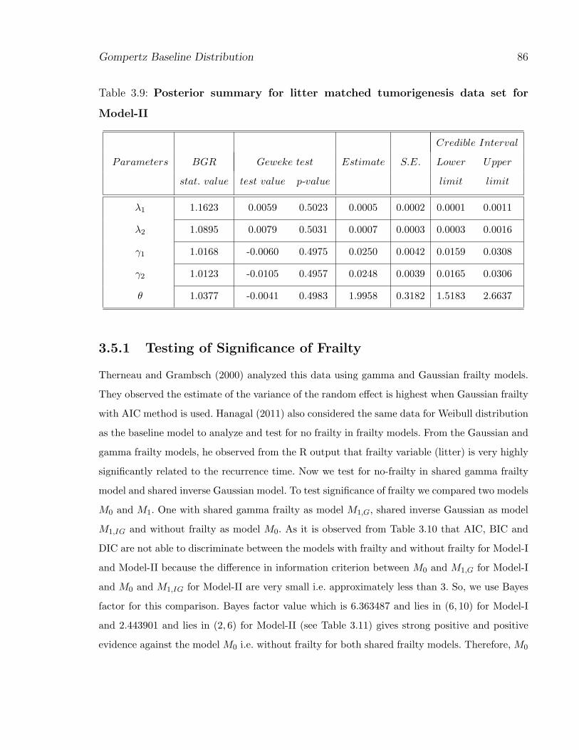
There is little difference between the posterior estimates of baseline parameters γ1, γ2 and
frailty parameter θ for Model-I and Model-II, presented in Tables 3.8 and 3.9. The posterior
estimate of dispersion of random effects i.e. θ = 1.9875 for Model-I and θ = 1.9958 for Model-II,
shows that there exists highly significant heterogeneity in population of rats. Thus, there is a
dependence within the litter.
Gompertz Baseline Distribution 86
Table 3.9: Posterior summary for litter matched tumorigenesis data set for
Model-II
Credible Interval
Parameters BGR Geweke test Estimate S.E. Lower Upper
stat. value test value p-value limit limit
λ1 1.1623 0.0059 0.5023 0.0005 0.0002 0.0001 0.0011
λ2 1.0895 0.0079 0.5031 0.0007 0.0003 0.0003 0.0016
γ1 1.0168 -0.0060 0.4975 0.0250 0.0042 0.0159 0.0308
γ2 1.0123 -0.0105 0.4957 0.0248 0.0039 0.0165 0.0306
θ 1.0377 -0.0041 0.4983 1.9958 0.3182 1.5183 2.6637
3.5.1 Testing of Significance of Frailty
Therneau and Grambsch (2000) analyzed this data using gamma and Gaussian frailty models.
They observed the estimate of the variance of the random effect is highest when Gaussian frailty
with AIC method is used. Hanagal (2011) also considered the same data for Weibull distribution
as the baseline model to analyze and test for no frailty in frailty models. From the Gaussian and
gamma frailty models, he observed from the R output that frailty variable (litter) is very highly
significantly related to the recurrence time. Now we test for no-frailty in shared gamma frailty
model and shared inverse Gaussian model. To test significance of frailty we compared two models
M0 and M1. One with shared gamma frailty as model M1,G, shared inverse Gaussian as model
M1,IG and without frailty as model M0. As it is observed from Table 3.10 that AIC, BIC and
DIC are not able to discriminate between the models with frailty and without frailty for Model-I
and Model-II because the difference in information criterion between M0 and M1,G for Model-I
and M0 and M1,IG for Model-II are very small i.e. approximately less than 3. So, we use Bayes
factor for this comparison. Bayes factor value which is 6.363487 and lies in (6, 10) for Model-I
and 2.443901 and lies in (2, 6) for Model-II (see Table 3.11) gives strong positive and positive
evidence against the model M0 i.e. without frailty for both shared frailty models. Therefore, M0

Gompertz Baseline Distribution 87
is worse than M1 based on Bayes factor and all other criterion. Thus, it is observed from the
results that frailty variable i.e litter effect is very highly significantly related to the recurrence
time of rats.
Table 3.10: AIC, BIC and DIC values for test of significance for frailty under
Model-I & Model-II fitted to litter matched tumorigenesis data set
Models Frailty AIC AICc BIC DIC log-likelihood
I with (M1,G) 267.649 269.014 279.114 261.457 -128.825
II with (M1,IG) 266.3979 267.7615 278.2191 260.9202 -128.1989
I&II without (M0) 265.2342 266.123 275.2299 261.9294 -128.6171
Table 3.11: Bayes factor values and decision for test of significance for frailty
under Model-I & Model-II fitted to litter matched tumorigenesis data set
numerator model
Models against 2loge(B10) range Evidence against
denominator model model in denominator
I M1,G against M0 6.363487 ≥ 6 and ≤ 10 Strong Positive
II M1,IG against M0 2.443901 ≥ 2and ≤ 6 Positive
3.6 Discussion
In this Chapter, shared gamma frailty model and shared inverse Gaussian frailty model with
Gompertz baseline distribution has been introduced. We have developed the Bayesian estimation
procedure to estimate the parameters of the models. Firstly we have considered simulation study
to see the performance of the models and then applied to the litter matched tumorigenesis data.
In case of simulation, we have chosen the gamma as prior distribution to check the effect of sample
Gompertz Baseline Distribution 88
size on the posterior estimates. It was observed from all results of Tables and Figures that the
posterior summary estimates with gamma prior assumptions were close to true parameter values.
In this Chapter, we have considered the litter matched tumorigenesis experiment study. Here,
we have discussed the Bayesian estimation procedure including Gibbs sampling for computing
the estimation of the unknown parameters for litter matched tumorigenesis data set. For this
data set we have no covariate as we have considered only controlled rats and also, we were
mainly interested to see the effect of frailty. We have discussed Kolmogorov-Smirnov statistical
tests for testing goodness-of-fit to Gompertz distribution. K-S test gives the statistical evidence
of not rejecting the hypotheses that data follows Gompertz baseline distribution.
For estimation purpose, we have run two parallel chains with two sets of priors from different
starting points and considered the “burn-in” interval for each chain. We have provided 95,000
iterations to perform the analysis. We have clearly written the steps involved in the iteration
procedure, using R-program, given in Appendix B. The quality of convergence was checked
graphically by trace plots and running mean plots and statistically by Geweke test statistics
and Gelman-Rubin statistics (see Brooks and Gelman, 1998). The values of the Gelman-Rubin
statistics in this case are quite close to one. Thus, the sample can be considered to have arisen
from stationary distribution. Thus, all convergence diagnostics suggest that the MCMC chains
are mixing very well, converging to a value, and attain stationary distribution.
We have given the complete posterior summary of the data set including posterior mean,
standard error, and 95% credible interval for both shared frailty models. We have compared
the model with frailty and model without frailty using some information criteria such as, log-
likelihood, AIC, AICc, BIC, DIC, and Bayes factor for both shared frailty models. From the
value of all these criteria we conclude that the shared frailty model provide a suitable choice
for modeling the life time model of litter matched tumorigenesis data as compared to without
frailty model. From the tests for heterogeneity and posterior estimates of frailty parameter set
we can conclude that there is highly significant heterogeneity among the rats. Data analysis of
tumorigenesis experiment indicates that the performance of Bayesian estimation method is quite
satisfactory.


![Frailty pathway [970kb]](https://img.pdfslide.us/doc/110x75/588da5761a28ab737b8b4e2c/frailty-pathway-970kb.jpg)


![Classes of Ordinary Differential Equations Obtained for ... · distribution [19], bivariate Gompertz [20], Gompertz-power . Abstract — In this paper, the differential calculus was](https://img.pdfslide.us/doc/110x75/5c0865ae09d3f23a458c07be/classes-of-ordinary-differential-equations-obtained-for-distribution-19.jpg)