Embed Size (px)
Citation preview

Chapter 3
Expectation
CHAPTER OUTLINE
Section 1 The Discrete CaseSection 2 The Absolutely Continuous CaseSection 3 Variance, Covariance and CorrelationSection 4 Generating FunctionsSection 5 Conditional ExpectationSection 6 InequalitiesSection 7 General Expectations (Advanced)Section 8 Further Proofs (Advanced)
In the first two chapters we learned about probability models, random variables, anddistributions. There is one more concept that is fundamental to all of probability theory,that of expected value.
Intuitively, the expected value of a random variable is the average value that therandom variable takes on. For example, if half the time X = 0, and the other half ofthe time X = 10, then the average value of X is 5. We shall write this as E(X) = 5.Similarly, if one-third of the time Y = 6 while two-thirds of the time Y = 15, thenE(Y ) = 12.
Another interpretation of expected value is in terms of fair gambling. Supposesomeone offers you a ticket (e.g., a lottery ticket) worth a certain random amount X .How much would you be willing to pay to buy the ticket? It seems reasonable that youwould be willing to pay the expected value E(X) of the ticket, but no more. However,this interpretation does have certain limitations; see Example 3.1.12.
To understand expected value more precisely, we consider discrete and absolutelycontinuous random variables separately.
3.1 The Discrete CaseWe begin with a definition.
129

130 Section 3.1: The Discrete Case
Definition 3.1.1 Let X be a discrete random variable. Then the expected value (ormean value or mean) of X , written E(X) (or µX ), is defined by
E(X) =x∈R1
x P(X = x) =x∈R1
x pX (x).
We will have P(X = x) = 0 except for those values x that are possible values of X .Hence, an equivalent definition is the following.
Definition 3.1.2 Let X be a discrete random variable, taking on distinct valuesx1, x2, . . . , with pi = P(X = xi ). Then the expected value of X is given by
E(X) =i
xi pi .
The definition (in either form) is best understood through examples.
EXAMPLE 3.1.1Suppose, as above, that P(X = 0) = P(X = 10) = 1/2. Then
E(X) = (0)(1/2)+ (10)(1/2) = 5,
as predicted.
EXAMPLE 3.1.2Suppose, as above, that P(Y = 6) = 1/3, and P(Y = 15) = 2/3. Then
E(Y ) = (6)(1/3)+ (15)(2/3) = 2+ 10 = 12,
again as predicted.
EXAMPLE 3.1.3Suppose that P(Z = −3) = 0.2, and P(Z = 11) = 0.7, and P(Z = 31) = 0.1. Then
E(Z) = (−3)(0.2)+ (11)(0.7)+ (31)(0.1) = −0.6+ 7.7+ 3.1 = 10.2.
EXAMPLE 3.1.4Suppose that P(W = −3) = 0.2, and P(W = −11) = 0.7, and P(W = 31) = 0.1.Then
E(W) = (−3)(0.2)+ (−11)(0.7)+ (31)(0.1) = −0.6− 7.7+ 3.1 = −5.2.
In this case, the expected value of W is negative.
We thus see that, for a discrete random variable X , once we know the probabilities thatX = x (or equivalently, once we know the probability function pX ), it is straightfor-ward (at least in simple cases) to compute the expected value of X .
We now consider some of the common discrete distributions introduced in Sec-tion 2.3.

Chapter 3: Expectation 131
EXAMPLE 3.1.5 Degenerate DistributionsIf X ≡ c is a constant, then P(X = c) = 1, so
E(X) = (c)(1) = c,
as it should.
EXAMPLE 3.1.6 The Bernoulli(θ) Distribution and Indicator FunctionsIf X ∼ Bernoulli(θ), then P(X = 1) = θ and P(X = 0) = 1− θ , so
E(X) = (1)(θ)+ (0)(1− θ) = θ.As a particular application of this, suppose we have a response s taking values in a
sample S and A ⊂ S. Letting X (s) = IA (s) , we have that X is the indicator functionof the set A and so takes the values 0 and 1. Then we have that P(X = 1) = P (A) ,and so X ∼ Bernoulli(P (A)) . This implies that
E (X) = E (IA) = P(A).
Therefore, we have shown that the expectation of the indicator function of the set A isequal to the probability of A.
EXAMPLE 3.1.7 The Binomial(n, θ) DistributionIf Y ∼ Binomial(n, θ), then
P(Y = k) = n
kθk(1− θ)n−k
for k = 0, 1, . . . , n. Hence,
E(Y ) =n
k=0
k P(Y = k) =n
k=0
kn
kθk(1− θ)n−k
=n
k=0
kn!
k! (n − k)!θk(1− θ)n−k =
n
k=1
n!(k − 1)! (n − k)!
θk(1− θ)n−k
=n
k=1
n (n − 1)!(k − 1)! (n − k)!
θk(1− θ)n−k =n
k=1
nn − 1k − 1
θk(1− θ)n−k .
Now, the binomial theorem says that for any a and b and any positive integer m,
(a + b)m =m
j=0
m
ja jbm− j .
Using this, and setting j = k − 1, we see that
E(Y ) =n
k=1
nn − 1
k − 1θk(1− θ)n−k =
n−1
j=0
nn − 1
jθ j+1(1− θ)n− j−1
= nθn−1
j=0
n − 1j
θ j (1− θ)n− j−1 = nθ (θ + 1− θ)n−1 = nθ.

132 Section 3.1: The Discrete Case
Hence, the expected value of Y is nθ . Note that this is precisely n times the ex-pected value of X , where X ∼ Bernoulli(θ) as in Example 3.1.6. We shall see inExample 3.1.15 that this is not a coincidence.
EXAMPLE 3.1.8 The Geometric(θ) DistributionIf Z ∼ Geometric(θ), then P(Z = k) = (1− θ)kθ for k = 0, 1, 2, . . . . Hence,
E(Z) =∞
k=0
k(1− θ)kθ. (3.1.1)
Therefore, we can write
(1− θ)E(Z) =∞
=0
(1− θ) +1θ.
Using the substitution k = + 1, we compute that
(1− θ)E(Z) =∞
k=1
(k − 1) (1− θ)kθ. (3.1.2)
Subtracting (3.1.2) from (3.1.1), we see that
θE(Z) = (E(Z))− ((1− θ)E(Z)) =∞
k=1
(k − (k − 1)) (1− θ)kθ
=∞
k=1
(1− θ)kθ = 1− θ1− (1− θ)θ = 1− θ.
Hence, θE(Z) = 1− θ , and we obtain E(Z) = (1− θ)/θ .
EXAMPLE 3.1.9 The Poisson(λ) DistributionIf X ∼ Poisson(λ), then P(X = k) = e−λλk/k! for k = 0, 1, 2, . . . . Hence, setting= k − 1,
E(X) =∞
k=0
ke−λ λk
k!=
∞
k=1
e−λ λk
(k − 1)!= λe−λ
∞
k=1
λk−1
(k − 1)!
= λ e−λ∞
=0
λ
!= λ e−λeλ = λ,
and we conclude that E(X) = λ.
It should be noted that expected values can sometimes be infinite, as the followingexample demonstrates.
EXAMPLE 3.1.10Let X be a discrete random variable, with probability function pX given by
pX (2k) = 2−k

Chapter 3: Expectation 133
for k = 1, 2, 3, . . . , with pX (x) = 0 for other values of x . That is, pX (2) = 1/2,pX (4) = 1/4, pX (8) = 1/8, etc., while pX (1) = pX (3) = pX (5) = pX (6) = · · · = 0.
Then it is easily checked that pX is indeed a valid probability function (i.e., pX (x) ≥0 for all x , with x pX (x) = 1). On the other hand, we compute that
E(X) =∞
k=1
(2k)(2−k) =∞
k=1
(1) =∞.
We therefore say that E(X) =∞, i.e., that the expected value of X is infinite.
Sometimes the expected value simply does not exist, as in the following example.
EXAMPLE 3.1.11Let Y be a discrete random variable, with probability function pY given by
pY (y) = 1/2y y = 2, 4, 8, 16, . . .
1/2|y| y = −2,−4,−8,−16, . . .0 otherwise.
That is, pY (2) = pY (−2) = 1/4, pY (4) = pY (−4) = 1/8, pY (8) = pY (−8) =1/16, etc. Then it is easily checked that pY is indeed a valid probability function (i.e.,pY (y) ≥ 0 for all y, with y pY (y) = 1).
On the other hand, we compute that
E(Y ) =y
y pY (y) =∞
k=1
(2k)(1/2 2k)+∞
k=1
(−2k)(1/2 2k)
=∞
k=1
(1/2)−∞
k=1
(1/2) =∞−∞,
which is undefined. We therefore say that E(Y ) does not exist, i.e., that the expectedvalue of Y is undefined in this case.
EXAMPLE 3.1.12 The St. Petersburg ParadoxSuppose someone makes you the following deal. You will repeatedly flip a fair coinand will receive an award of 2Z pennies, where Z is the number of tails that appearbefore the first head. How much would you be willing to pay for this deal?
Well, the probability that the award will be 2z pennies is equal to the probability thatyou will flip z tails and then one head, which is equal to 1/2z+1. Hence, the expectedvalue of the award (in pennies) is equal to
∞
z=0
(2z)(1/2z+1) =∞
z=0
1/2 =∞.
In words, the average amount of the award is infinite!Hence, according to the “fair gambling” interpretation of expected value, as dis-
cussed at the beginning of this chapter, it seems that you should be willing to pay aninfinite amount (or, at least, any finite amount no matter how large) to get the award

134 Section 3.1: The Discrete Case
promised by this deal! How much do you think you should really be willing to pay forit?1
EXAMPLE 3.1.13 The St. Petersburg Paradox, TruncatedSuppose in the St. Petersburg paradox (Example 3.1.12), it is agreed that the award willbe truncated at 230 cents (which is just over $10 million!). That is, the award will bethe same as for the original deal, except the award will be frozen once it exceeds 230
cents. Formally, the award is now equal to 2min(30,Z) pennies, where Z is as before.How much would you be willing to pay for this new award? Well, the expected
value of the new award (in cents) is equal to
∞
z=1
(2min(30,z))(1/2z+1) =30
z=1
(2z)(1/2z+1)+∞
z=31
(230)(1/2z+1)
=30
z=1
(1/2)+ (230)(1/231) = 31/2 = 15.5.
That is, truncating the award at just over $10 million changes its expected value enor-mously, from infinity to less than 16 cents!
In utility theory, it is often assumed that each person has a utility function U suchthat, if they win x cents, their amount of “utility” (i.e., benefit or joy or pleasure) isequal to U(x). In this context, the truncation of Example 3.1.13 may be thought ofnot as changing the rules of the game but as corresponding to a utility function of theform U(x) = min(x, 230). In words, this says that your utility is equal to the amountof money you get, until you reach 230 cents (approximately $10 million), after whichpoint you don’t care about money2 anymore. The result of Example 3.1.13 then saysthat, with this utility function, the St. Petersburg paradox is only worth 15.5 cents toyou — even though its expected value is infinite.
We often need to compute expected values of functions of random variables. For-tunately, this is not too difficult, as the following theorem shows.
Theorem 3.1.1(a) Let X be a discrete random variable, and let g : R1 → R1 be some function
such that the expectation of the random variable g(X) exists. Then
E (g(X)) =x
g(x) P(X = x).
(b) Let X and Y be discrete random variables, and let h : R2 → R1 be somefunction such that the expectation of the random variable h(X, Y ) exists. Then
E (h(X,Y )) =x,y
h(x, y)P(X = x, Y = y).
1When one of the authors first heard about this deal, he decided to try it and agreed to pay $1. In fact, hegot four tails before the first head, so his award was 16 cents, but he still lost 84 cents overall.
2Or, perhaps, you think it is unlikely you will be able to collect the money!

Chapter 3: Expectation 135
PROOF We prove part (b) here. Part (a) then follows by simply setting h(x, y) =g(x) and noting that
x,yg(x) P(X = x, Y = y) =
xg(x) P(X = x).
Let Z = h(X,Y ).We have that
E(Z) =z
z P(Z = z) =z
z P(h(X, Y ) = z)
=z
zx,y
h(x,y)=z
P(X = x, Y = y) =x,y z
z=h(x,y)
z P(X = x, Y = y)
=x,y
h(x, y) P(X = x, Y = y),
as claimed.
One of the most important properties of expected value is that it is linear, stated asfollows.
Theorem 3.1.2 (Linearity of expected values) Let X and Y be discrete randomvariables, let a and b be real numbers, and put Z = aX + bY . Then E(Z) =aE(X)+ bE(Y ).
PROOF Let pX,Y be the joint probability function of X and Y . Then using Theo-rem 3.1.1,
E(Z) =x,y(ax + by) pX,Y (x, y) = a
x,yx pX,Y (x, y)+ b
x,yy pX,Y (x, y)
= ax
xy
pX,Y (x, y)+ by
yx
pX,Y (x, y).
Because y pX,Y (x, y) = pX (x) and x pX,Y (x, y) = pY (y), we have that
E(Z) = ax
x pX (x)+ by
y pY (y) = aE(X)+ bE(Y ),
as claimed.
EXAMPLE 3.1.14Let X ∼ Binomial(n, θ1), and let Y ∼ Geometric(θ2). What is E(3X − 2Y )?
We already know (Examples 3.1.6 and 3.1.7) that E(X) = n θ1 and E(Y ) = (1−θ2) / θ2. Hence, by Theorem 3.1.2, E(3X − 2Y ) = 3E(X)− 2E(Y ) = 3nθ1 − 2(1−θ2)/θ2.
EXAMPLE 3.1.15Let Y ∼ Binomial(n, θ). Then we know (cf. Example 2.3.3) that we can think ofY = X1 + · · · + Xn, where each Xi ∼ Bernoulli(θ) (in fact, Xi = 1 if the i th coin is

136 Section 3.1: The Discrete Case
heads, otherwise Xi = 0). Because E(Xi ) = θ for each i , it follows immediately fromTheorem 3.1.2 that
E(Y ) = E(X1)+ · · · + E(Xn) = θ + · · · + θ = nθ.
This gives the same answer as Example 3.1.7, but much more easily.
Suppose that X is a random variable and Y = c is a constant. Then from Theorem3.1.2, we have that E(X + c) = E(X) + c. From this we see that the mean value µXof X is a measure of the location of the probability distribution of X. For example, ifX takes the value x with probability p and the value y with probability 1− p, then themean of X is µX = px + (1− p)y which is a value between x and y. For a constant c,the probability distribution of X + c is concentrated on the points x+c and y+ c, withprobabilities p and 1− p, respectively. The mean of X+c is µX+c,which is betweenthe points x + c and y + c, i.e., the mean shifts with the probability distribution. It isalso true that if X is concentrated on the finite set of points x1 < x2 < · · · < xk, thenx1 ≤ µX ≤ xk, and the mean shifts exactly as we shift the distribution. This is depictedin Figure 3.1.1 for a distribution concentrated on k = 4 points. Using the results ofSection 2.6.1, we have that pX+c(x) = pX (x − c).
x1 x2 x3 x4
pX
•E(X)
x1+c x2+c x3+c x4+c•
E(X+c)
pX+c
Figure 3.1.1: The probability functions and means of discrete random variables X and X + c.
Theorem 3.1.2 says, in particular, that E(X + Y ) = E(X) + E(Y ), i.e., that ex-pectation preserves sums. It is reasonable to ask whether the same property holds forproducts. That is, do we necessarily have E(XY ) = E(X)E(Y )? In general, theanswer is no, as the following example shows.

Chapter 3: Expectation 137
EXAMPLE 3.1.16Let X and Y be discrete random variables, with joint probability function given by
pX,Y (x, y) =
1/2 x = 3, y = 51/6 x = 3, y = 91/6 x = 6, y = 51/6 x = 6, y = 90 otherwise.
Then
E(X) =x
x P(X = x) = (3)(1/2+ 1/6)+ (6)(1/6+ 1/6) = 4
and
E(Y ) =y
y P(Y = y) = (5)(1/2+ 1/6)+ (9)(1/6+ 1/6) = 19/3,
while
E(XY ) =z
z P(XY = z)
= (3)(5)(1/2)+ (3)(9)(1/6)+ (6)(5)(1/6)+ (6)(9)(1/6)= 26.
Because (4)(19/3) = 26, we see that E(X) E(Y ) = E(XY ) in this case.
On the other hand, if X and Y are independent, then we do have E(X)E(Y ) =E(XY ).
Theorem 3.1.3 Let X and Y be discrete random variables that are independent.Then E(XY ) = E(X)E(Y ).
PROOF Independence implies (see Theorem 2.8.3) that P(X = x, Y = y) =P(X = x) P(Y = y). Using this, we compute by Theorem 3.1.1 that
E(XY ) =x,y
xy P(X = x, Y = y) =x,y
xy P(X = x) P(Y = y)
=x
x P(X = x)y
y P(Y = y) = E(X) E(Y ),
as claimed.
Theorem 3.1.3 will be used often in subsequent chapters, as will the following impor-tant property.
Theorem 3.1.4 (Monotonicity) Let X and Y be discrete random variables, andsuppose that X ≤ Y . (Remember that this means X (s) ≤ Y (s) for all s ∈ S.) ThenE(X) ≤ E(Y ).
138 Section 3.1: The Discrete Case
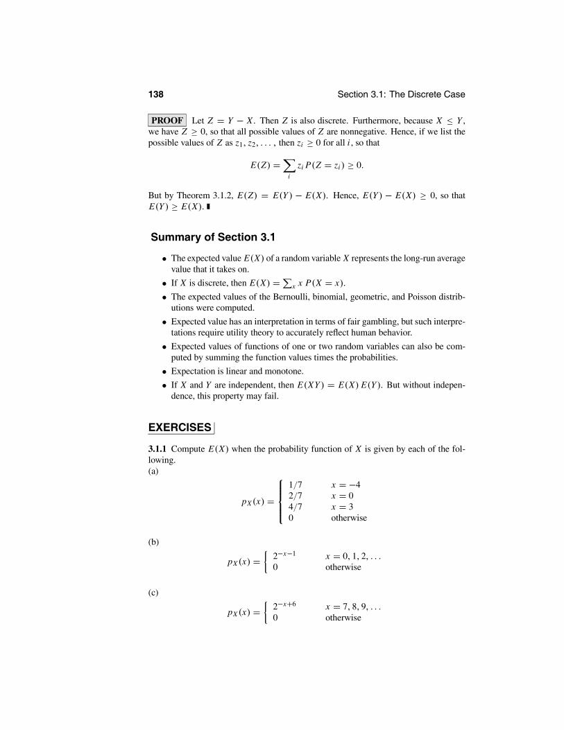
PROOF Let Z = Y − X . Then Z is also discrete. Furthermore, because X ≤ Y ,we have Z ≥ 0, so that all possible values of Z are nonnegative. Hence, if we list thepossible values of Z as z1, z2, . . . , then zi ≥ 0 for all i , so that
E(Z) =i
zi P(Z = zi ) ≥ 0.
But by Theorem 3.1.2, E(Z) = E(Y ) − E(X). Hence, E(Y ) − E(X) ≥ 0, so thatE(Y ) ≥ E(X).
Summary of Section 3.1
• The expected value E(X) of a random variable X represents the long-run averagevalue that it takes on.
• If X is discrete, then E(X) = x x P(X = x).
• The expected values of the Bernoulli, binomial, geometric, and Poisson distrib-utions were computed.
• Expected value has an interpretation in terms of fair gambling, but such interpre-tations require utility theory to accurately reflect human behavior.
• Expected values of functions of one or two random variables can also be com-puted by summing the function values times the probabilities.
• Expectation is linear and monotone.
• If X and Y are independent, then E(XY ) = E(X) E(Y ). But without indepen-dence, this property may fail.
EXERCISES
3.1.1 Compute E(X) when the probability function of X is given by each of the fol-lowing.(a)
pX (x) =
1/7 x = −42/7 x = 04/7 x = 30 otherwise
(b)
pX (x) = 2−x−1 x = 0, 1, 2, . . .0 otherwise
(c)
pX (x) = 2−x+6 x = 7, 8, 9, . . .0 otherwise

Chapter 3: Expectation 139
3.1.2 Let X and Y have joint probability function given by
pX,Y (x, y) =
1/7 x = 5, y = 01/7 x = 5, y = 31/7 x = 5, y = 43/7 x = 8, y = 01/7 x = 8, y = 40 otherwise,
as in Example 2.7.5. Compute each of the following.(a) E(X)(b) E(Y )(c) E(3X + 7Y )(d) E(X2)(e) E(Y 2)(f) E(XY )(g) E(XY + 14)3.1.3 Let X and Y have joint probability function given by
pX,Y (x, y) =
1/2 x = 2, y = 101/6 x = −7, y = 101/12 x = 2, y = 121/12 x = −7, y = 121/12 x = 2, y = 141/12 x = −7, y = 140 otherwise.
Compute each of the following.(a) E(X).(b) E(Y )(c) E(X2)(d) E(Y 2)(e) E(X2 + Y 2)(f) E(XY − 4Y )
3.1.4 Let X ∼ Bernoulli(θ1) and Y ∼ Binomial(n, θ2). Compute E(4X − 3Y ).3.1.5 Let X ∼ Geometric(θ) and Y ∼ Poisson(λ). Compute E(8X − Y + 12).3.1.6 Let Y ∼ Binomial(100, 0.3), and Z ∼ Poisson(7). Compute E(Y + Z).3.1.7 Let X ∼ Binomial(80, 1/4), and let Y ∼ Poisson(3/2). Assume X and Y areindependent. Compute E(XY ).3.1.8 Starting with one penny, suppose you roll one fair six-sided die and get paid anadditional number of pennies equal to three times the number showing on the die. LetX be the total number of pennies you have at the end. Compute E(X).3.1.9 Suppose you start with eight pennies and flip one fair coin. If the coin comes upheads, you get to keep all your pennies; if the coin comes up tails, you have to givehalf of them back. Let X be the total number of pennies you have at the end. ComputeE(X).

140 Section 3.1: The Discrete Case
3.1.10 Suppose you flip two fair coins. Let Y = 3 if the two coins show the sameresult, otherwise let Y = 5. Compute E(Y ).3.1.11 Suppose you roll two fair six-sided dice.(a) Let Z be the sum of the two numbers showing. Compute E(Z).(b) Let W be the product of the two numbers showing. Compute E(W ).3.1.12 Suppose you flip one fair coin and roll one fair six-sided die. Let X be theproduct of the numbers of heads (i.e., 0 or 1) times the number showing on the die.Compute E(X). (Hint: Do not forget Theorem 3.1.3.)3.1.13 Suppose you roll one fair six-sided die and then flip as many coins as the num-ber showing on the die. (For example, if the die shows 4, then you flip four coins.) LetY be the number of heads obtained. Compute E(Y ).3.1.14 Suppose you roll three fair coins, and let X be the cube of the number of headsshowing. Compute E(X).
PROBLEMS
3.1.15 Suppose you start with one penny and repeatedly flip a fair coin. Each time youget heads, before the first time you get tails, you get two more pennies. Let X be thetotal number of pennies you have at the end. Compute E(X).3.1.16 Suppose you start with one penny and repeatedly flip a fair coin. Each time youget heads, before the first time you get tails, your number of pennies is doubled. Let Xbe the total number of pennies you have at the end. Compute E(X).3.1.17 Let X ∼ Geometric(θ), and let Y = min(X, 100).(a) Compute E(Y ).(b) Compute E(Y − X).3.1.18 Give an example of a random variable X such that E min(X, 100) = E(X).3.1.19 Give an example of a random variable X such that E(min(X, 100)) = E(X)/2.3.1.20 Give an example of a joint probability function pX,Y for random variables Xand Y , such that X ∼ Bernoulli(1/4) and Y ∼ Bernoulli(1/2), but E(XY ) = 1/8.3.1.21 For X ∼ Hypergeometric(N,M, n), prove that E(X) = nM/N .
3.1.22 For X ∼ Negative-Binomial (r, θ), prove that E(X) = r(1 − θ)/θ. (Hint:Argue that if X1, . . . , Xr are independent and identically distributed Geometric(θ) ,then X = X1 + · · · + Xr ∼ Negative-Binomial(r, θ) .)3.1.23 Suppose that (X1, X2, X3) ∼Multinomial(n, θ1, θ2, θ3) . Prove thatE(Xi ) = nθ i .
CHALLENGES
3.1.24 Let X ∼ Geometric(θ). Compute E(X2).3.1.25 Suppose X is a discrete random variable, such that E (min(X, M)) = E(X).Prove that P(X > M) = 0.

Chapter 3: Expectation 141
DISCUSSION TOPICS
3.1.26 How much would you be willing to pay for the deal corresponding to the St. Pe-tersburg paradox (see Example 3.1.12)? Justify your answer.3.1.27 What utility function U (as in the text following Example 3.1.13) best describesyour own personal attitude toward money? Why?
3.2 The Absolutely Continuous CaseSuppose now that X is absolutely continuous, with density function fX . How canwe compute E(X) then? By analogy with the discrete case, we might try computing
x x P(X = x), but because P(X = x) is always zero, this sum is always zero aswell.
On the other hand, if is a small positive number, then we could try approximatingE(X) by
E(X) ≈i
i P(i ≤ X < (i + 1) ),
where the sum is over all integers i . This makes sense because, if is small andi ≤ X < (i + 1) , then X ≈ i .
Now, we know that
P(i ≤ X < (i + 1) ) =(i+1)
ifX (x) dx.
This tells us that
E(X) ≈i
(i+1)
ii fX (x) dx.
Furthermore, in this integral, i ≤ x < (i + 1) . Hence, i ≈ x . We therefore see that
E(X) ≈i
(i+1)
ix fX (x) dx =
∞
−∞x fX (x) dx .
This prompts the following definition.
Definition 3.2.1 Let X be an absolutely continuous random variable, with densityfunction fX . Then the expected value of X is given by
E(X) =∞
−∞x fX (x) dx.
From this definition, it is not too difficult to compute the expected values of manyof the standard absolutely continuous distributions.

142 Section 3.2: The Absolutely Continuous Case
EXAMPLE 3.2.1 The Uniform[0, 1] DistributionLet X ∼ Uniform[0, 1] so that the density of X is given by
fX (x) = 1 0 ≤ x ≤ 10 otherwise.
Hence,
E(X) =∞
−∞x fX (x) dx =
1
0x dx = x2
2
x=1
x=0= 1/2,
as one would expect.
EXAMPLE 3.2.2 The Uniform[L, R] DistributionLet X ∼ Uniform[L, R] so that the density of X is given by
fX (x) = 1/(R − L) L ≤ x ≤ R0 otherwise.
Hence,
E(X) =∞
−∞x fX (x) dx =
R
Lx
1R − L
dx = x2
2(R − L)
x=R
x=L
= R2 − L2
2(R − L)= (R − L)(R + L)
2(R − L)= R + L
2,
again as one would expect.
EXAMPLE 3.2.3 The Exponential(λ) DistributionLet Y ∼ Exponential(λ) so that the density of Y is given by
fY (y) = λe−λy y ≥ 00 y < 0.
Hence, integration by parts, with u = y and dv = λ e−λy (so du = dy, v = −e−λy),leads to
E(Y ) =∞
−∞y fY (y) dy =
∞
0y λ e−λy dy = − ye−λy ∞0 +
∞
0e−λy dy
=∞
0e−λy dy = − e−λy
λ
∞
0= −0− 1
λ= 1
λ.
In particular, if λ = 1, then Y ∼ Exponential(1), and E(Y ) = 1.
EXAMPLE 3.2.4 The N(0, 1) DistributionLet Z ∼ N(0, 1) so that the density of Z is given by
fZ (z) = φ(z) = 1√2π
e−z2/2.

Chapter 3: Expectation 143
Hence,
E(Z) =∞
−∞z fZ (z) dz
=∞
−∞z
1√2π
e−z2/2 dz
=0
−∞z
1√2π
e−z2/2 dz +∞
0z
1√2π
e−z2/2 dz. (3.2.1)
But using the substitution w = −z, we see that
0
−∞z
1√2π
e−z2/2 dz =∞
0(−w) 1√
2πe−w2/2 dw.
Then the two integrals in (3.2.1) cancel each other out, and leaving us with E(Z) = 0.
As with discrete variables, means of absolutely continuous random variables canalso be infinite or undefined.
EXAMPLE 3.2.5Let X have density function given by
fX (x) = 1/x2 x ≥ 10 otherwise.
Then
E(X) =∞
−∞x fX (x) dx =
∞
1x (1/x2) dx =
∞
1(1/x) dx = log x
x=∞x=1
=∞.
Hence, the expected value of X is infinite.
EXAMPLE 3.2.6Let Y have density function given by
fY (y) = 1/2y2 y ≥ 1
1/2y2 y ≤ −10 otherwise.
Then
E(Y ) =∞
−∞y fY (y) dy =
−1
−∞y(1/y2) dy +
∞
1y(1/y2) dy
= −∞
1(1/y) dy +
∞
1(1/y) dy = −∞+∞,
which is undefined. Hence, the expected value of Y is undefined (i.e., does not exist)in this case.

144 Section 3.2: The Absolutely Continuous Case
Theorem 3.1.1 remains true in the continuous case, as follows.
Theorem 3.2.1(a) Let X be an absolutely continuous random variable, with density function fX ,and let g : R1 → R1 be some function. Then when the expectation of g(X) exists,
E (g(X)) =∞
−∞g(x) fX (x) dx .
(b) Let X and Y be jointly absolutely continuous random variables, with joint den-sity function fX,Y , and let h : R2 → R1 be some function. Then when the expecta-tion of h(X,Y ) exists,
E (h(X, Y )) =∞
−∞
∞
−∞h(x, y) fX,Y (x, y) dx dy.
We do not prove Theorem 3.2.1 here; however, we shall use it often. For a first useof this result, we prove that expected values for absolutely continuous random variablesare still linear.
Theorem 3.2.2 (Linearity of expected values) Let X and Y be jointly absolutelycontinuous random variables, and let a and b be real numbers. Then E(aX+bY ) =aE(X)+ bE(Y ).
PROOF Let fX,Y be the joint density function of X and Y . Then using Theo-rem 3.2.1, we compute that
E(Z) =∞
−∞
∞
−∞(ax + by) fX,Y (x, y) dx dy
= a∞
−∞
∞
−∞x fX,Y (x, y) dx dy + b
∞
−∞
∞
−∞y fX,Y (x, y) dx dy
= a∞
−∞x
∞
−∞fX,Y (x, y) dy dx
+b∞
−∞y
∞
−∞fX,Y (x, y) dx dy.
But ∞−∞ fX,Y (x, y) dy = fX (x) and ∞
−∞ fX,Y (x, y) dx = fY (y), so
E(Z) = a∞
−∞x fX (x) dx + b
∞
−∞y fY (y) dy = aE(X)+ bE(Y ),
as claimed.
Just as in the discrete case, we have that E(X + c) = E(X) + c for an absolutelycontinuous random variable X. Note, however, that this is not implied by Theorem3.2.2 because the constant c is a discrete, not absolutely continuous, random variable.

Chapter 3: Expectation 145
In fact, we need a more general treatment of expectation to obtain this result (see Sec-tion 3.7). In any case, the result is true and we again have that the mean of a randomvariable serves as a measure of the location of the probability distribution of X. InFigure 3.2.1, we have plotted the densities and means of the absolutely continuous ran-dom variables X and X + c. The change of variable results from Section 2.6.2 givefX+c(x) = fX (x − c) .
•E(X)
•E(X+c)
fX
fX+c
x
x
Figure 3.2.1: The densities and means of absolutely continuous random variables X andX + c.
EXAMPLE 3.2.7 The N(µ, σ 2) DistributionLet X ∼ N(µ, σ 2). Then we know (cf. Exercise 2.6.3) that if Z = (X − µ) / σ , thenZ ∼ N(0, 1). Hence, we can write X = µ+ σ Z , where Z ∼ N(0, 1). But we know(see Example 3.2.4) that E(Z) = 0 and (Example 3.1.5) that E(µ) = µ. Hence, usingTheorem 3.2.2, E(X) = E(µ+ σ Z) = E(µ)+ σ E(Z) = µ+ σ (0) = µ.
If X and Y are independent, then the following results show that we again haveE(XY ) = E(X) E(Y ).
Theorem 3.2.3 Let X and Y be jointly absolutely continuous random variables thatare independent. Then E(XY ) = E(X)E(Y ).
PROOF Independence implies (Theorem 2.8.3) that fX,Y (x, y) = fX (x) fY (y).Using this, along with Theorem 3.2.1, we compute
E(XY ) =∞
−∞
∞
−∞xy fX,Y (x, y) dx dy =
∞
−∞
∞
−∞xy fX (x) fY (y) dx dy
=∞
−∞x fX (x) dx
∞
−∞y fY (y) dy = E(X)E(Y ),
as claimed.

146 Section 3.2: The Absolutely Continuous Case
The monotonicity property (Theorem 3.1.4) still holds as well.
Theorem 3.2.4 (Monotonicity) Let X and Y be jointly continuous random vari-ables, and suppose that X ≤ Y . Then E(X) ≤ E(Y ).
PROOF Let fX,Y be the joint density function of X and Y . Because X ≤ Y , thedensity fX,Y can be chosen so that fX,Y (x, y) = 0 whenever x > y. Now let Z =Y − X . Then by Theorem 3.2.1(b),
E(Z) =∞
−∞
∞
−∞(y − x) fX,Y (x, y) dx dy .
Because fX,Y (x, y) = 0 whenever x > y, this implies that E(Z) ≥ 0. But by Theo-rem 3.2.2, E(Z) = E(Y )− E(X). Hence, E(Y )− E(X) ≥ 0, so that E(Y ) ≥ E(X).
Summary of Section 3.2
• If X is absolutely continuous, then E(X) = x fX (x) dx .
• The expected values of the uniform, exponential, and normal distributions werecomputed.
• Expectation for absolutely continuous random variables is linear and monotone.
• If X and Y are independent, then we still have E(XY ) = E(X) E(Y ).
EXERCISES
3.2.1 Compute C and E(X) when the density function of X is given by each of thefollowing.(a)
fX (x) = C 5 ≤ x ≤ 90 otherwise
(b)
fX (x) = C(x + 1) 6 ≤ x ≤ 80 otherwise
(c)
fX (x) = Cx4 −5 ≤ x ≤ −20 otherwise
3.2.2 Let X and Y have joint density
fX,Y (x, y) = 4x2y + 2y5 0 ≤ x ≤ 1 , 0 ≤ y ≤ 10 otherwise,
as in Examples 2.7.6 and 2.7.7. Compute each of the following.(a) E(X)
Chapter 3: Expectation 147
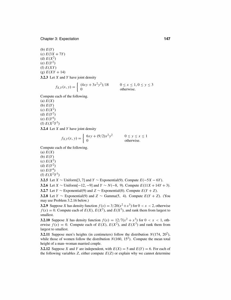
(b) E(Y )(c) E(3X + 7Y )(d) E(X2)(e) E(Y 2)(f) E(XY )(g) E(XY + 14)3.2.3 Let X and Y have joint density
fX,Y (x, y) = (4xy + 3x2y2)/18 0 ≤ x ≤ 1, 0 ≤ y ≤ 30 otherwise.
Compute each of the following.(a) E(X)(b) E(Y )(c) E(X2)(d) E(Y 2)(e) E(Y 4)(f) E(X2Y 3)
3.2.4 Let X and Y have joint density
fX,Y (x, y) = 6xy + (9/2)x2y2 0 ≤ y ≤ x ≤ 10 otherwise.
Compute each of the following.(a) E(X)(b) E(Y )(c) E(X2)(d) E(Y 2)(e) E(Y 4)(f) E(X2Y 3)
3.2.5 Let X ∼ Uniform[3, 7] and Y ∼ Exponential(9). Compute E(−5X − 6Y ).3.2.6 Let X ∼ Uniform[−12,−9] and Y ∼ N(−8, 9). Compute E(11X + 14Y + 3).3.2.7 Let Y ∼ Exponential(9) and Z ∼ Exponential(8). Compute E(Y + Z).3.2.8 Let Y ∼ Exponential(9) and Z ∼ Gamma(5, 4). Compute E(Y + Z). (Youmay use Problem 3.2.16 below.)3.2.9 Suppose X has density function f (x) = 3/20(x2+x3) for 0 < x < 2, otherwisef (x) = 0. Compute each of E(X), E(X2), and E(X3), and rank them from largest tosmallest.3.2.10 Suppose X has density function f (x) = 12/7(x2 + x3) for 0 < x < 1, oth-erwise f (x) = 0. Compute each of E(X), E(X2), and E(X3) and rank them fromlargest to smallest.3.2.11 Suppose men’s heights (in centimeters) follow the distribution N(174, 202),while those of women follow the distribution N(160, 152). Compute the mean totalheight of a man–woman married couple.3.2.12 Suppose X and Y are independent, with E(X) = 5 and E(Y ) = 6. For each ofthe following variables Z , either compute E(Z) or explain why we cannot determine

148 Section 3.2: The Absolutely Continuous Case
E(Z) from the available information:(a) Z = X + Y(b) Z = XY(c) Z = 2X − 4Y(d) Z = 2X (3+ 4Y )(e) Z = (2+ X)(3+ 4Y )(f) Z = (2+ X)(3X + 4Y )
3.2.13 Suppose darts are randomly thrown at a wall. Let X be the distance (in cen-timeters) from the left edge of the dart’s point to the left end of the wall, and let Y bethe distance from the right edge of the dart’s point to the left end of the wall. Assumethe dart’s point is 0.1 centimeters thick, and that E(X) = 214. Compute E(Y ).3.2.14 Let X be the mean height of all citizens measured from the top of their head,and let Y be the mean height of all citizens measured from the top of their head or hat(whichever is higher). Must we have E(Y ) ≥ E(X)? Why or why not?3.2.15 Suppose basketball teams A and B each have five players and that each memberof team A is being “guarded” by a unique member of team B. Suppose it is noticed thateach member of team A is taller than the corresponding gusrf from team B. Does itnecessarily follow that the mean height of team A is larger than the mean height ofteam B? Why or why not?
PROBLEMS
3.2.16 Let α > 0 and λ > 0, and let X ∼ Gamma(α, λ). Prove that E(X) = α/λ.(Hint: The computations are somewhat similar to those of Problem 2.4.15. You willalso need property (2.4.7) of the gamma function.)3.2.17 Suppose that X follows the logistic distribution (see Problem 2.4.18). Provethat E(X) = 0.3.2.18 Suppose that X follows the Weibull(α) distribution (see Problem 2.4.19). Provethat E(X) = α−1 + 1 .
3.2.19 Suppose that X follows the Pareto(α) distribution (see Problem 2.4.20) for α >1. Prove that E(X) = 1/ (α − 1) .What is E(X) when 0 < α ≤ 1?3.2.20 Suppose that X follows the Cauchy distribution (see Problem 2.4.21). Arguethat E(X) does not exist. (Hint: Compute the integral in two parts, where the integrandis positive and where the integrand is negative.)3.2.21 Suppose that X follows the Laplace distribution (see Problem 2.4.22). Provethat E(X) = 0.3.2.22 Suppose that X follows the Beta(a, b) distribution (see Problem 2.4.24). Provethat E(X) = a/(a + b).
3.2.23 Suppose that (X1, X2) ∼ Dirichlet(α1, α2, α3) (see Problem 2.7.17). Provethat E(Xi ) = αi/ (α1 + α2 + α3) .

Chapter 3: Expectation 149
3.3 Variance, Covariance, and CorrelationNow that we understand expected value, we can use it to define various other quantitiesof interest. The numerical values of these quantities provide information about thedistribution of random variables.
Given a random variable X , we know that the average value of X will be E(X).However, this tells us nothing about how far X tends to be from E(X). For that, wehave the following definition.
Definition 3.3.1 The variance of a random variable X is the quantity
σ 2x = Var(X) = E (X − µX )
2 , (3.3.1)
where µX = E(X) is the mean of X .
We note that it is also possible to write (3.3.1) as Var(X) = E (X − E(X))2 ; how-ever, the multiple uses of “E” may be confusing. Also, because (X − µX )
2 is alwaysnonnegative, its expectation is always defined, so the variance of X is always defined.
Intuitively, the variance Var(X) is a measure of how spread out the distribution ofX is, or how random X is, or how much X varies, as the following example illustrates.
EXAMPLE 3.3.1Let X and Y be two discrete random variables, with probability functions
pX (x) = 1 x = 100 otherwise
and
pY (y) = 1/2 y = 5
1/2 y = 150 otherwise,
respectively.Then E(X) = E(Y ) = 10. However,
Var(X) = (10− 10)2(1) = 0,
whileVar(Y ) = (5− 10)2(1/2)+ (15− 10)2(1/2) = 25.
We thus see that, while X and Y have the same expected value, the variance of Y ismuch greater than that of X . This corresponds to the fact that Y is more random thanX ; that is, it varies more than X does.

150 Section 3.3: Variance, Covariance, and Correlation
EXAMPLE 3.3.2Let X have probability function given by
pX (x) =
1/2 x = 21/6 x = 31/6 x = 41/6 x = 50 otherwise.
Then E(X) = (2)(1/2)+ (3)(1/6)+ (4)(1/6)+ (5)(1/6) = 3. Hence,
Var(X) = ((2− 3)2)12+ ((3− 3)2)
16+ ((4− 3)2)
16+ ((5− 3)2)
16= 4/3.
EXAMPLE 3.3.3Let Y ∼ Bernoulli(θ). Then E(Y ) = θ . Hence,
Var(Y ) = E((Y − θ)2) = ((1− θ)2)(θ)+ ((0− θ)2)(1− θ)= θ − 2θ2 + θ3 + θ2 − θ3 = θ − θ2 = θ(1− θ).
The square in (3.3.1) implies that the “scale” of Var(X) is different from the scaleof X . For example, if X were measuring a distance in meters (m), then Var(X) wouldbe measuring in meters squared (m2). If we then switched from meters to feet, wewould have to multiply X by about 3.28084 but would have to multiply Var(X) byabout (3.28084)2.
To correct for this “scale” problem, we can simply take the square root, as follows.
Definition 3.3.2 The standard deviation of a random variable X is the quantity
σ X = Sd(X) = Var(X) = E((X − µX )2).
It is reasonable to ask why, in (3.3.1), we need the square at all. Now, if we simplyomitted the square and considered E((X − µX )), we would always get zero (becauseµX = E(X)), which is useless. On the other hand, we could instead use E(|X −µX |).This would, like (3.3.1), be a valid measure of the average distance of X from µX .Furthermore, it would not have the “scale problem” that Var(X) does. However, weshall see that Var(X) has many convenient properties. By contrast, E(|X − µX |) isvery difficult to work with. Thus, it is purely for convenience that we define varianceby E((X − µX )
2) instead of E(|X − µX |).Variance will be very important throughout the remainder of this book. Thus, we
pause to present some important properties of Var.
Theorem 3.3.1 Let X be any random variable, with expected value µX = E(X),and variance Var(X). Then the following hold true:(a) Var(X) ≥ 0.(b) If a and b are real numbers, Var(aX + b) = a2 Var(X).(c) Var(X) = E(X2)− (µX )
2 = E(X2)− E(X)2. (That is, variance is equal to thesecond moment minus the square of the first moment.)(d) Var(X) ≤ E(X2).

Chapter 3: Expectation 151
PROOF (a) This is immediate, because we always have (X − µX )2 ≥ 0.
(b) We note that µaX+b = E(aX + b) = aE(X)+ b = aµX + b, by linearity. Hence,again using linearity,
Var(aX + b) = E (aX + b − µaX+b)2 = E (aX + b− aµX + b)2
= a2E (X − µX )2 = a2 Var(X).
(c) Again, using linearity,
Var(X) = E (X − µX )2 = E X2 − 2XµX + (µX )
2
= E(X2)− 2E(X)µX + (µX )2 = E(X2)− 2(µX )
2 + (µX )2
= E(X2)− (µX )2.
(d) This follows immediately from part (c) because we have −(µX )2 ≤ 0.
Theorem 3.3.1 often provides easier ways of computing variance, as in the follow-ing examples.
EXAMPLE 3.3.4 Variance of the Exponential(λ) DistributionLet W ∼ Exponential(λ), so that fW (w) = λe−λw. Then E(W ) = 1/λ. Also, usingintegration by parts,
E(W 2) =∞
0w2λe−λwdw =
∞
02we−λwdw
= (2/λ)∞
0wλe−λwdw = (2/λ)E(W ) = 2/λ2.
Hence, by part (c) of Theorem 3.3.1,
Var(W ) = E(W 2)− (E(W ))2 = (2/λ2)− (1/λ)2 = 1/λ2.
EXAMPLE 3.3.5Let W ∼ Exponential(λ), and let Y = 5W + 3. Then from the above example,Var(W ) = 1/λ2. Then, using part (b) of Theorem 3.3.1,
Var(Y ) = Var(5W + 3) = 25 Var(W ) = 25/λ2.
Because√
a2 = |a|, part (b) of Theorem 3.3.1 immediately implies a correspond-ing fact about standard deviation.
Corollary 3.3.1 Let X be any random variable, with standard deviation Sd(X), andlet a be any real number. Then Sd(aX) = |a|Sd(X).
EXAMPLE 3.3.6Let W ∼ Exponential(λ), and let Y ∼ 5W + 3. Then using the above examples, wesee that Sd(W) = (Var(W ))1/2 = 1/λ2 1/2 = 1/λ. Also, Sd(Y ) = (Var(Y ))1/2 =25/λ2 1/2 = 5/λ. This agrees with Corollary 3.3.1, since Sd(Y ) = |5|Sd(W ).

152 Section 3.3: Variance, Covariance, and Correlation
EXAMPLE 3.3.7 Variance and Standard Deviation of the N(µ, σ 2) DistributionSuppose that X ∼ N(µ, σ 2). In Example 3.2.7 we established that E (X) = µ. Nowwe compute Var(X) .
First consider Z ∼ N(0, 1). Then from Theorem 3.3.1(c) we have that
Var (Z) = E Z2 =∞
−∞z2 1√
2πexp − z2
2dz.
Then, putting u = z, dv = z exp −z2/2 (so du = 1, v = − exp −z2/2 ), and usingintegration by parts, we obtain
Var (Z) = − 1√2π
z exp −z2/2∞
−∞+
∞
−∞1√2π
exp − z2
2dz = 1
and Sd(Z) = 1.Now, for σ > 0, put X = µ+ σ Z . We then have X ∼ N(µ, σ 2). From Theorem
3.3.1(b) we have that
Var (X) = Var (µ+ σ Z) = σ 2 Var (Z) = σ 2
and Sd(X) = σ. This establishes the variance of the N(µ, σ 2) distribution as σ 2 andthe standard deviation as σ.
In Figure 3.3.1, we have plotted three normal distributions, all with mean 0 butdifferent variances.
-5 -4 -3 -2 -1 0 1 2 3 4 5
0.2
0.4
0.6
0.8
1.0
x
f
Figure 3.3.1: Plots of the the N(0, 1) (solid line), the N(0, 1/4) (dashed line) and theN(0, 4) (dotted line) density functions.
The effect of the variance on the amount of spread of the distribution about the meanis quite clear from these plots. As σ 2 increases, the distribution becomes more diffuse;as it decreases, it becomes more concentrated about the mean 0.
So far we have considered the variance of one random variable at a time. How-ever, the related concept of covariance measures the relationship between two randomvariables.

Chapter 3: Expectation 153
Definition 3.3.3 The covariance of two random variables X and Y is given by
Cov(X,Y ) = E ((X − µX )(Y − µY )) ,
where µX = E(X) and µY = E(Y ).
EXAMPLE 3.3.8Let X and Y be discrete random variables, with joint probability function pX,Y givenby
pX,Y (x, y) =
1/2 x = 3, y = 41/3 x = 3, y = 61/6 x = 5, y = 60 otherwise.
Then E(X) = (3)(1/2) + (3)(1/3) + (5)(1/6) = 10/3, and E(Y ) = (4)(1/2) +(6)(1/3)+ (6)(1/6) = 5. Hence,
Cov(X, Y ) = E((X − 10/3)(Y − 5))
= (3− 10/3) (4− 5)/2+ (3− 10/3) (6− 5)/3+ (5− 10/3) (6− 5)/6
= 1/3.
EXAMPLE 3.3.9Let X be any random variable with Var(X) > 0. Let Y = 3X , and let Z = −4X . ThenµY = 3µX and µZ = −4µX . Hence,
Cov(X, Y ) = E((X − µX )(Y − µY )) = E((X − µX )(3X − 3µX ))
= 3 E((X − µX )2) = 3 Var(X),
while
Cov(X, Z) = E((X − µX )(Z − µZ )) = E((X − µX )((−4)X − (−4)µX ))
= (−4)E((X − µX )2) = −4 Var(X).
Note in particular that Cov(X,Y ) > 0, while Cov(X, Z) < 0. Intuitively, this says thatY increases when X increases, whereas Z decreases when X increases.
We begin with some simple facts about covariance. Obviously, we always haveCov(X, Y ) =Cov(Y, X).We also have the following result.
Theorem 3.3.2 (Linearity of covariance) Let X , Y , and Z be three random vari-ables. Let a and b be real numbers. Then
Cov(aX + bY, Z) = a Cov(X, Z)+ b Cov(Y, Z).

154 Section 3.3: Variance, Covariance, and Correlation
PROOF Note that by linearity, µaX+bY ≡ E(aX + bY ) = aE(X) + bE(Y ) ≡aµX + bµY . Hence,
Cov(aX + bY, Z) = E (aX + bY − µaX+bY )(Z − µZ )
= E ((aX + bY − aµX − bµY )(Z − µZ ))
= E ((aX − aµX + bY − bµY )(Z − µZ ))
= aE ((X − µX )(Z − µZ ))+ bE ((Y − µY )(Z − µZ ))
= a Cov(X, Z)+ b Cov(Y, Z),
and the result is established.
We also have the following identity, which is similar to Theorem 3.3.1(c).
Theorem 3.3.3 Let X and Y be two random variables. Then
Cov(X, Y ) = E(XY )− E(X)E(Y ).
PROOF Using linearity, we have
Cov(X,Y ) = E ((X − µX )(Y − µY )) = E (XY − µXY − XµY + µXµY )
= E(XY )− µX E(Y )− E(X)µY + µXµY
= E(XY )− µXµY − µXµY + µXµY = E(XY )− µXµY .
Corollary 3.3.2 If X and Y are independent, then Cov(X, Y ) = 0.
PROOF Because X and Y are independent, we know (Theorems 3.1.3 and 3.2.3)that E(XY ) = E(X) E(Y ). Hence, the result follows immediately from Theorem 3.3.3.
We note that the converse to Corollary 3.3.2 is false, as the following exampleshows.
EXAMPLE 3.3.10 Covariance 0 Does Not Imply Independence.Let X and Y be discrete random variables, with joint probability function pX,Y givenby
pX,Y (x, y) =
1/4 x = 3, y = 51/4 x = 4, y = 91/4 x = 7, y = 51/4 x = 6, y = 90 otherwise.
Then E(X) = (3)(1/4) + (4)(1/4) + (7)(1/4) + (6)(1/4) = 5, E(Y ) = (5)(1/4) +(9)(1/4) + (5)(1/4) + (9)(1/4) = 7, and E(XY ) = (3)(5)(1/4) + (4)(9)(1/4) +(7)(5)(1/4) + (6)(9)(1/4) = 35. We obtain Cov(X,Y ) = E(XY ) − E(X) E(Y ) =35− (5)(7) = 0.
Chapter 3: Expectation 155
On the other hand, X and Y are clearly not independent. For example, P(X =4) > 0 and P(Y = 5) > 0, but P(X = 4, Y = 5) = 0, so P(X = 4, Y = 5) =P(X = 4) P(Y = 5).
There is also an important relationship between variance and covariance.
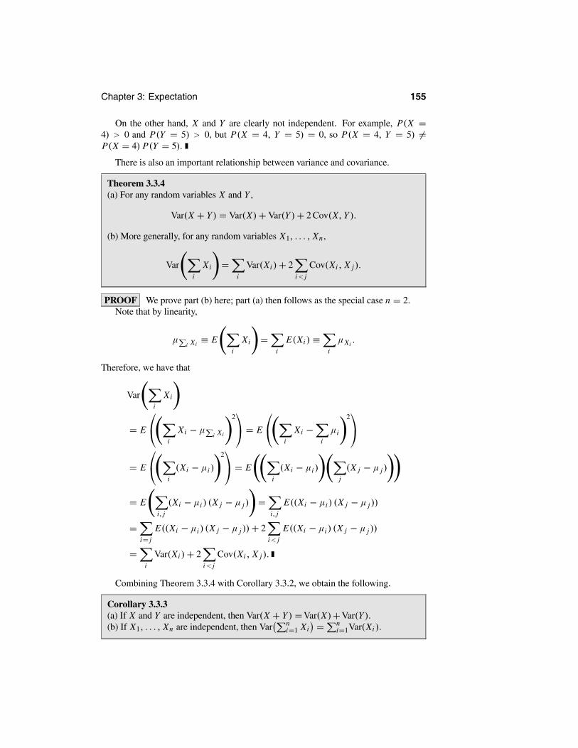
Theorem 3.3.4(a) For any random variables X and Y ,
Var(X + Y ) = Var(X)+ Var(Y )+ 2 Cov(X, Y ).
(b) More generally, for any random variables X1, . . . , Xn ,
Vari
Xi =i
Var(Xi )+ 2i< j
Cov(Xi , X j).
PROOF We prove part (b) here; part (a) then follows as the special case n = 2.Note that by linearity,
µi Xi
≡ Ei
Xi =i
E(Xi ) ≡i
µXi.
Therefore, we have that
Vari
Xi
= E
i
Xi − µ i Xi
2 = E
i
Xi −i
µi
2
= E
i
(Xi − µi )
2 = E
i
(Xi − µi )j
(X j − µ j )
= Ei, j
(Xi − µi ) (X j − µ j ) =i, j
E((Xi − µi ) (X j − µ j ))
=i= j
E((Xi − µi ) (X j − µ j ))+ 2i< j
E((Xi − µi ) (X j − µ j ))
=i
Var(Xi )+ 2i< j
Cov(Xi , X j ).
Combining Theorem 3.3.4 with Corollary 3.3.2, we obtain the following.
Corollary 3.3.3(a) If X and Y are independent, then Var(X + Y ) =Var(X)+Var(Y ).(b) If X1, . . . , Xn are independent, then Var n
i=1 Xi = ni=1Var(Xi ).

156 Section 3.3: Variance, Covariance, and Correlation
One use of Corollary 3.3.3 is the following.
EXAMPLE 3.3.11Let Y ∼ Binomial(n, θ). What is Var(Y )? Recall that we can write
Y = X1 + X2 + · · · + Xn,
where the Xi are independent, with Xi ∼ Bernoulli(θ). We have already seen thatVar(Xi ) = θ(1− θ). Hence, from Corollary 3.3.3,
Var(Y ) = Var(X1)+Var(X2)+ · · · + Var(Xn)
= θ(1− θ)+ θ(1− θ)+ · · · + θ(1− θ) = nθ(1− θ).Another concept very closely related to covariance is correlation.
Definition 3.3.4 The correlation of two random variables X and Y is given by
Corr(X,Y ) = Cov(X, Y )Sd(X)Sd(Y )
= Cov(X, Y )√Var(X)Var(Y )
provided Var(X) <∞ and Var(Y ) <∞.EXAMPLE 3.3.12As in Example 3.3.2, let X be any random variable with Var(X) > 0, let Y = 3X , andlet Z = −4X . Then Cov(X,Y ) = 3 Var(X) and Cov(X, Z) = −4 Var(X). But byCorollary 3.3.1, Sd(Y ) = 3 Sd(X) and Sd(Z) = 4 Sd(X). Hence,
Corr(X, Y ) = Cov(X,Y )Sd(X)Sd(Y )
= 3 Var(X)Sd(X)3 Sd(X)
= Var(X)
Sd(X)2= 1,
because Sd(X)2 = Var(X). Also, we have that
Corr(X, Z) = Cov(X, Z)Sd(X)Sd(Z)
= −4 Var(X)Sd(X)4 Sd(X)
= −Var(X)
Sd(X)2= −1.
Intuitively, this again says that Y increases when X increases, whereas Z decreaseswhen X increases. However, note that the scale factors 3 and −4 have cancelled out;only their signs were important.
We shall see later, in Section 3.6, that we always have −1 ≤Corr(X,Y ) ≤ 1, forany random variables X and Y . Hence, in Example 3.3.12, Y has the largest possiblecorrelation with X (which makes sense because Y increases whenever X does, withoutexception), while Z has the smallest possible correlation with X (which makes sensebecause Z decreases whenever X does). We will also see that Corr(X, Y ) is a measureof the extent to which a linear relationship exists between X and Y .
EXAMPLE 3.3.13 The Bivariate Normal(µ1, µ2, σ 1, σ 2, ρ) DistributionWe defined this distribution in Example 2.7.9. It turns out that when (X,Y ) follows thisjoint distribution then, (from Problem 2.7.13) X ∼ N(µ1, σ
21) and Y ∼ N(µ2, σ
22).
Further, we have that (see Problem 3.3.17) Corr(X,Y ) = ρ. In the following graphs,

Chapter 3: Expectation 157
we have plotted samples of n = 1000 values of (X, Y ) from bivariate normal distrib-utions with µ1 = µ2 = 0, σ 2
1 = σ 22 = 1, and various values of ρ. Note that we used
(2.7.1) to generate these samples.From these plots we can see the effect of ρ on the joint distribution. Figure 3.3.2
shows that when ρ = 0, the point cloud is roughly circular. It becomes elliptical inFigure 3.3.3 with ρ = 0.5, and more tightly concentrated about a line in Figure 3.3.4with ρ = 0.9. As we will see in Section 3.6, the points will lie exactly on a line whenρ = 1.
Figure 3.3.5 demonstrates the effect of a negative correlation. With positive corre-lations, the value of Y tends to increase with X, as reflected in the upward slope of thepoint cloud. With negative correlations, Y tends to decrease with X, as reflected in thenegative slope of the point cloud.
543210-1-2-3-4-5
4
3
2
1
0
-1
-2
-3
-4
X
Y
Figure 3.3.2: A sample of n = 1000 values (X,Y ) from the Bivariate Normal (0, 0, 1, 1, 0)distribution.
543210-1-2-3-4-5
4
3
2
1
0
-1
-2
-3
-4
X
Y
Figure 3.3.3: A sample of n = 1000 values (X, Y ) from the Bivariate Normal(0, 0, 1, 1, 0.5) distribution.

158 Section 3.3: Variance, Covariance, and Correlation
543210-1-2-3-4-5
4
3
2
1
0
-1
-2
-3
-4
X
YFigure 3.3.4: A sample of n = 1000 values (X,Y ) from the Bivariate Normal(0, 0, 1, 1, 0.9) distribution.
543210-1-2-3-4-5
4
3
2
1
0
-1
-2
-3
-4
X
Y
Figure 3.3.5: A sample of n = 1000 values (X,Y ) from the Bivariate Normal(0, 0, 1, 1,−0.9) distribution.
Summary of Section 3.3
• The variance of a random variable X measures how far it tends to be from itsmean and is given by Var(X) = E((X − µX )
2) = E(X2)− (E(X))2.
• The variances of many standard distributions were computed.
• The standard deviation of X equals Sd(X) = √Var(X).
• Var(X) ≥ 0, and Var(aX + b) = a2 Var(X); also Sd(aX + b) = |a|Sd(X).
• The covariance of random variables X and Y measures how they are related andis given by Cov(X,Y ) = E((X − µX )(Y − µy)) = E(XY )− E(X) E(Y ).
• If X and Y are independent, then Cov(X,Y ) = 0.
• Var(X + Y ) =Var(X)+Var(Y ) + 2 Cov(X,Y ). If X and Y are independent,this equals Var(X)+Var(Y ) .
• The correlation of X and Y is Corr(X, Y ) =Cov(X,Y )/(Sd(X)Sd(Y )).

Chapter 3: Expectation 159
EXERCISES
3.3.1 Suppose the joint probability function of X and Y is given by
pX,Y (x, y) =
1/2 x = 3, y = 51/6 x = 3, y = 91/6 x = 6, y = 51/6 x = 6, y = 90 otherwise,
with E(X) = 4, E(Y ) = 19/3, and E(XY ) = 26, as in Example 3.1.16.(a) Compute Cov(X, Y ).(b) Compute Var(X) and Var(Y ).(c) Compute Corr(X,Y ).3.3.2 Suppose the joint probability function of X and Y is given by
pX,Y (x, y) =
1/7 x = 5, y = 01/7 x = 5, y = 31/7 x = 5, y = 43/7 x = 8, y = 01/7 x = 8, y = 40 otherwise,
as in Example 2.7.5.(a) Compute E(X) and E(Y ).(b) Compute Cov(X, Y ).(c) Compute Var(X) and Var(Y ).(d) Compute Corr(X, Y ).3.3.3 Let X and Y have joint density
fX,Y (x, y) = 4x2y + 2y5 0 ≤ x ≤ 1, 0 ≤ y ≤ 10 otherwise,
as in Exercise 3.2.2. Compute Corr(X,Y ).3.3.4 Let X and Y have joint density
fX,Y (x, y) = 15x3y4 + 6x2y7 0 ≤ x ≤ 1, 0 ≤ y ≤ 10 otherwise.
Compute E(X), E(Y ), Var(X), Var(Y ), Cov(X,Y ), and Corr(X,Y ).3.3.5 Let Y and Z be two independent random variables, each with positive variance.Prove that Corr(Y, Z) = 0.3.3.6 Let X , Y , and Z be three random variables, and suppose that X and Z are inde-pendent. Prove that Cov(X + Y, Z) =Cov(Y, Z).3.3.7 Let X ∼ Exponential(3) and Y ∼ Poisson(5). Assume X and Y are independent.Let Z = X + Y .(a) Compute Cov(X, Z).(b) Compute Corr(X, Z).

160 Section 3.3: Variance, Covariance, and Correlation
3.3.8 Prove that the variance of the Uniform[L, R] distribution is given by the expres-sion (R − L)2/12.3.3.9 Prove that Var(X) = E(X (X − 1)) − E(X)E(X − 1). Use this to computedirectly from the probability function that when X ∼ Binomial(n, θ), then Var(X) =nθ (1− θ) .3.3.10 Suppose you flip three fair coins. Let X be the number of heads showing, andlet Y = X2. Compute E(X), E(Y ), Var(X), Var(Y ), Cov(X, Y ), and Corr(X, Y ).3.3.11 Suppose you roll two fair six-sided dice. Let X be the number showing on thefirst die, and let Y be the sum of the numbers showing on the two dice. Compute E(X),E(Y ), E(XY ), and Cov(X, Y ).3.3.12 Suppose you flip four fair coins. Let X be the number of heads showing, andlet Y be the number of tails showing. Compute Cov(X,Y ) and Corr(X, Y ).3.3.13 Let X and Y be independent, with X ∼Bernoulli(1/2) and Y ∼Bernoulli(1/3).Let Z = X + Y and W = X − Y . Compute Cov(Z,W) and Corr(Z,W ).3.3.14 Let X and Y be independent, with X ∼ Bernoulli(1/2) and Y ∼ N(0, 1). LetZ = X+Y and W = X−Y . Compute Var(Z), Var(W ), Cov(Z,W ), and Corr(Z,W).3.3.15 Suppose you roll one fair six-sided die and then flip as many coins as the num-ber showing on the die. (For example, if the die shows 4, then you flip four coins.) LetX be the number showing on the die, and Y be the number of heads obtained. ComputeCov(X,Y ).
PROBLEMS
3.3.16 Let X ∼ N (0, 1), and let Y = cX .(a) Compute limc 0 Cov(X,Y ).(b) Compute limc 0 Cov(X, Y ).(c) Compute limc 0 Corr(X,Y ).(d) Compute limc 0 Corr(X, Y ).(e) Explain why the answers in parts (c) and (d) are not the same.3.3.17 Let X and Y have the bivariate normal distribution, as in Example 2.7.9. Provethat Corr(X,Y ) = ρ. (Hint: Use (2.7.1).)3.3.18 Prove that the variance of the Geometric(θ) distribution is given by (1− θ) /θ2.(Hint: Use Exercise 3.3.9 and (1− θ)x = x (x − 1) (1− θ)x−2 .)3.3.19 Prove that the variance of the Negative-Binomial(r, θ) distribution is given byr(1− θ)/θ2. (Hint: Use Problem 3.3.18.)3.3.20 Let α > 0 and λ > 0, and let X ∼ Gamma(α, λ). Prove that Var(X) = α/λ2.(Hint: Recall Problem 3.2.16.)3.3.21 Suppose that X ∼ Weibull(α) distribution (see Problem 2.4.19). Prove thatVar(X) = (2/α + 1)− 2 (1/α + 1) . (Hint: Recall Problem 3.2.18.)3.3.22 Suppose that X ∼ Pareto(α) (see Problem 2.4.20) for α > 2. Prove thatVar(X) = α/((α − 1)2 (α − 2)). (Hint: Recall Problem 3.2.19.)3.3.23 Suppose that X follows the Laplace distribution (see Problem 2.4.22). Provethat Var(X) = 2. (Hint: Recall Problem 3.2.21.)

Chapter 3: Expectation 161
3.3.24 Suppose that X ∼ Beta(a, b) (see Problem 2.4.24). Prove that Var(X) =ab/((a + b)2(a + b+ 1)). (Hint: Recall Problem 3.2.22.)3.3.25 Suppose that (X1, X2, X3) ∼Multinomial(n, θ1, θ2, θ3). Prove that
Var(Xi ) = nθ i (1− θ i ), Cov(Xi , X j ) = −nθ iθ j , when i = j.
(Hint: Recall Problem 3.1.23.)3.3.26 Suppose that (X1, X2) ∼ Dirichlet(α1, α2, α3) (see Problem 2.7.17). Provethat
Var(Xi ) = αi (α1 + α2 + α3 − αi )
(α1 + α2 + α3)2 (α1 + α2 + α3 + 1)
,
Cov (X1, X2) = −α1α2
(α1 + α2 + α3)2 (α1 + α2 + α3 + 1)
.
(Hint: Recall Problem 3.2.23.)3.3.27 Suppose that X ∼ Hypergeometric(N,M, n). Prove that
Var(X) = nM
N1− M
N
N − n
N − 1.
(Hint: Recall Problem 3.1.21 and use Exercise 3.3.9.)3.3.28 Suppose you roll one fair six-sided die and then flip as many coins as the num-ber showing on the die. (For example, if the die shows 4, then you flip four coins.) LetX be the number showing on the die, and Y be the number of heads obtained. ComputeCorr(X, Y ).
CHALLENGES
3.3.29 Let Y be a nonnegative random variable. Prove that E(Y ) = 0 if and only ifP(Y = 0) = 1. (You may assume for simplicity that Y is discrete, but the result is truefor any Y .)3.3.30 Prove that Var(X) = 0 if and only if there is a real number c with P(X = c) =1. (You may use the result of Challenge 3.3.29.)3.3.31 Give an example of a random variable X , such that E(X) = 5, and Var(X) =∞.
3.4 Generating FunctionsLet X be a random variable. Recall that the cumulative distribution function of X ,defined by FX (x) = P(X ≤ x), contains all the information about the distribution ofX (see Theorem 2.5.1). It turns out that there are other functions — the probability-generating function and the moment-generating function — that also provide informa-tion (sometimes all the information) about X and its expected values.
Definition 3.4.1 Let X be a random variable (usually discrete). Then we define itsprobability-generating function, rX , by rX (t) = E(t X ) for t ∈ R1.

162 Section 3.4: Generating Functions
Consider the following examples of probability-generating functions.
EXAMPLE 3.4.1 The Binomial(n, θ) DistributionIf X ∼ Binomial(n, θ), then
rX (t) = E(t X ) =n
i=0
P(X = i)t i =n
i=0
n
iθ i(1− θ)n−i t i
=n
i=0
n
i(tθ)i (1− θ)n−i = (tθ + 1− θ)n,
using the binomial theorem.
EXAMPLE 3.4.2 The Poisson(λ) DistributionIf Y ∼ Poisson(λ), then
rY (t) = E(tY ) =∞
i=0
P(Y = i)t i =∞
i=0
e−λ λi
i!t i
=∞
i=0
e−λ (λt)i
i!= e−λeλt = eλ(t−1).
The following theorem tells us that once we know the probability-generating func-tion rX (t), then we can compute all the probabilities P(X = 0), P(X = 1), P(X = 2),etc.
Theorem 3.4.1 Let X be a discrete random variable, whose possible values are allnonnegative integers. Assume that rX (t0) <∞ for some t0 > 0. Then
rX (0) = P(X = 0),
rX (0) = P(X = 1),
rX (0) = 2 P(X = 2),
etc. In general,r (k)X (0) = k! P(X = k),
where r (k)X is the kth derivative of rX .
PROOF Because the possible values are all nonnegative integers of the form i =0, 1, 2, . . . , we have
rX (t) = E(t X ) =x
t x P(X = x) =∞
i=0
t i P(X = i)
= t0 P(X = 0)+ t1 P(X = 1)+ t2 P(X = 2)+ t3 P(X = 3)+ · · · ,so that
rX (t) = 1P(X = 0)+ t1 P(X = 1)+ t2 P(X = 2)+ t3 P(X = 3)+ · · · . (3.4.1)

Chapter 3: Expectation 163
Substituting t = 0 into (3.4.1), every term vanishes except the first one, and we obtainrX (0) = P(X = 0). Taking derivatives of both sides of (3.4.1), we obtain
rX (t) = 1P(X = 1)+ 2t1 P(X = 2)+ 3t2 P(X = 3)+ · · · ,and setting t = 0 gives rX (0) = P(X = 1). Taking another derivative of both sidesgives
rX (t) = 2P(X = 2)+ 3 · 2 t1 P(X = 3)+ · · ·and setting t = 0 gives rX (0) = 2 P(X = 2). Continuing in this way, we obtain thegeneral formula.
We now apply Theorem 3.4.1 to the binomial and Poisson distributions.
EXAMPLE 3.4.3 The Binomial(n, θ) DistributionFrom Example 3.4.1, we have that
rX (0) = (1− θ)nrX (0) = n(tθ + 1− θ)n−1(θ)
t=0= n(1− θ)n−1θ
rX (0) = n(n − 1)(tθ + 1− θ)n−2(θ)(θ)t=0= n(n − 1)(1− θ)n−2θ2,
etc. It is thus verified directly that
P(X = 0) = rX (0)
P(X = 1) = rX (0)
2 P(X = 2) = rX (0),
etc.
EXAMPLE 3.4.4 The Poisson(λ) DistributionFrom Example 3.4.2, we have that
rX (0) = e−λ
rX (0) = λe−λ
rX (0) = λ2e−λ,
etc. It is again verified that
P(X = 0) = rX (0)
P(X = 1) = rX (0)
2 P(X = 2) = rX (0),
etc.
From Theorem 3.4.1, we can see why rX is called the probability-generating func-tion. For, at least in the discrete case with the distribution concentrated on the non-negative integers, we can indeed generate the probabilities for X from rX . We thus

164 Section 3.4: Generating Functions
see immediately that for a random variable X that takes values only in {0, 1, 2, . . .},rX is unique. By this we mean that if X and Y are concentrated on {0, 1, 2, . . .} andrX = rY , then X and Y have the same distribution. This uniqueness property of theprobability-generating function can be very useful in trying to determine the distribu-tion of a random variable that takes only values in {0, 1, 2, . . .} .
It is clear that the probability-generating function tells us a lot — in fact, everything— about the distribution of random variables concentrated on the nonnegative integers.But what about other random variables? It turns out that there are other quantities,called moments, associated with random variables that are quite informative about theirdistributions.
Definition 3.4.2 Let X be a random variable, and let k be a positive integer. Thenthe kth moment of X is the quantity E(Xk), provided this expectation exists.
Note that if E(Xk) exists and is finite, it can be shown that E(Xl) exists and is finitewhen 0 ≤ l < k.
The first moment is just the mean of the random variable. This can be taken asa measure of where the central mass of probability for X lies in the real line, at leastwhen this distribution is unimodal (has a single peak) and is not too highly skewed. Thesecond moment E(X2), together with the first moment, gives us the variance throughVar(X) = E(X2)− (E(X))2 . Therefore, the first two moments of the distribution tellus about the location of the distribution and the spread, or degree of concentration, ofthat distribution about the mean. In fact, the higher moments also provide informationabout the distribution.
Many of the most important distributions of probability and statistics have all oftheir moments finite; in fact, they have what is called a moment-generating function.
Definition 3.4.3 Let X be any random variable. Then its moment-generating func-tion mX is defined by mX (s) = E(esX ) at s ∈ R1.
The following example computes the moment-generating function of a well-knowndistribution.
EXAMPLE 3.4.5 The Exponential(λ) DistributionLet X ∼ Exponential(λ). Then for s < λ,
mX (s) = E(esX ) =∞
−∞esx fX (x) dx =
∞
0esxλe−λx dx
=∞
0λ e(s−λ)x dx = λ e(s−λ)x
s − λx=∞x=0
= −λe(s−λ)0
s − λ= − λ
s − λ = λ(λ− s)−1.
A comparison of Definitions 3.4.1 and 3.4.3 immediately gives the following.
Theorem 3.4.2 Let X be any random variable. Then mX (s) = rX (es).

Chapter 3: Expectation 165
This result can obviously help us evaluate some moment-generating functions whenwe have rX already.
EXAMPLE 3.4.6Let Y ∼ Binomial(n, θ). Then we know that rY (t) = (tθ + 1− θ)n . Hence, mY (s) =rY (es) = (esθ + 1− θ)n .EXAMPLE 3.4.7Let Z ∼ Poisson(λ). Then we know that rZ (t) = eλ(t−1). Hence, mZ (s) = rZ (es) =eλ(e
s−1).
The following theorem tells us that once we know the moment-generating functionmX (t), we can compute all the moments E(X), E(X2), E(X3), etc.
Theorem 3.4.3 Let X be any random variable. Suppose that for some s0 > 0, it istrue that mX (s) <∞ whenever s ∈ (−s0, s0). Then
mX (0) = 1
mX (0) = E(X)
mX (0) = E(X2),
etc. In general,m(k)X (0) = E(Xk),
where m(k)X is the kth derivative of mX .
PROOF We know that mX (s) = E(esX ). We have
mX (0) = E(e0X ) = E(e0) = E(1) = 1.
Also, taking derivatives, we see3 that mX (s) = E(X esX ), so
mX (0) = E(X e0X ) = E(Xe0) = E(X).
Taking derivatives again, we see that mX (s) = E(X2esX ), so
mX (0) = E(X2 e0X ) = E(X2e0) = E(X2).
Continuing in this way, we obtain the general formula.
We now consider an application of Theorem 3.4.3.
EXAMPLE 3.4.8 The Mean and Variance of the Exponential(λ) DistributionUsing the moment-generating function computed in Example 3.4.5, we have
mX (s) = (−1)λ(λ− s)−2(−1) = λ(λ− s)−2.
3Strictly speaking, interchanging the order of derivative and expectation is justified by analytic functiontheory and requires that mX (s) <∞ whenever |s| < s0.

166 Section 3.4: Generating Functions
Therefore,E(X) = mX (0) = λ(λ− 0)−2 = λ/λ2 = 1/λ,
as it should. Also,
E(X2) = mX (0) = (−2)λ(λ− 0)−3(−1) = 2λ/λ3 = 2/λ2,
so we have
Var(X) = E(X2)− (E(X)) = (2/λ2)− (1/λ)2 = 1/λ2.
This provides an easy way of computing the variance of X .
EXAMPLE 3.4.9 The Mean and Variance of the Poisson(λ) DistributionIn Example 3.4.7, we obtained mZ (s) = exp (λ(es − 1)) . So we have
E(X) = mX (0) = λe0 exp λ(e0 − 1) = λ
E(X2) = mX (0) = λe0 exp λ(e0 − 1) + λe02
exp λ(e0 − 1) = λ+ λ2.
Therefore, Var(X) = E(X2)− (E(X))2 = λ+ λ2 − λ2 = λ.Computing the moment-generating function of a normal distribution is also impor-
tant, but it is somewhat more difficult.
Theorem 3.4.4 If X ∼ N(0, 1), then mX (s) = es2/2.
PROOF Because X has density φ(x) = (2π)−1/2 e−x2/2, we have that
mX (s) = E(esX ) =∞
−∞esxφ(x) dx =
∞
−∞esx 1√
2πe−x2/2 dx
= 1√2π
∞
−∞esx−(x2/2) dx = 1√
2π
∞
−∞e−(x−s)2/2+(s2/2) dx
= es2/2 1√2π
∞
−∞e−(x−s)2/2 dx.
Setting y = x − s (so that dy = dx), this becomes (using Theorem 2.4.2)
mX (s) = es2/2 1√2π
∞
−∞e−y2/2 dy = es2/2
∞
−∞φ(y) dy = es2/2,
as claimed.
One useful property of both probability-generating and moment-generating func-tions is the following.
Theorem 3.4.5 Let X and Y be random variables that are independent. Then wehave(a) rX+Y (t) = rX (t) rY (t), and(b) mX+Y (t) = mX (t)mY (t).

Chapter 3: Expectation 167
PROOF Because X and Y are independent, so are t X and tY (by Theorem 2.8.5).Hence, we know (by Theorems 3.1.3 and 3.2.3) that E(t X tY ) = E(t X ) E(tY ). Usingthis, we have
rX+Y (t) = E t X+Y = E t X tY = E(t X )E(tY ) = rX (t)rY (t).
Similarly,
mX+Y (t) = E et (X+Y ) = E etX etY = E(et X ) E(etY ) = mX (t)mY (t).
EXAMPLE 3.4.10Let Y ∼ Binomial(n, θ). Then, as in Example 3.1.15, we can write
Y = X1 + · · · + Xn,
where the {Xi } are i.i.d. with Xi ∼ Bernoulli(θ). Hence, Theorem 3.4.5 says we musthave rY (t) = rX1(t) rX2(t) · · · rXn (t). But for any i ,
rXi (t) =x
t x P(X = x) = t1θ + t0(1− θ) = θ t + 1− θ.
Hence, we must have
rY (t) = (θ t + 1− θ)(θ t + 1− θ) · · · (θ t + 1− θ) = (θ t + 1− θ)n,as already verified in Example 3.4.1.
Moment-generating functions, when defined in a neighborhood of 0, completelydefine a distribution in the following sense. (We omit the proof, which is advanced.)
Theorem 3.4.6 (Uniqueness theorem) Let X be a random variable, such that forsome s0 > 0, we have mX (s) < ∞ whenever s ∈ (−s0, s0). Then if Y is someother random variable with mY (s) = mX (s) whenever s ∈ (−s0, s0), then X and Yhave the same distribution.
Theorems 3.4.1 and 3.4.6 provide a powerful technique for identifying distribu-tions. For example, if we determine that the moment-generating function of X ismX (t) = exp s2/2 , then we know, from Theorems 3.4.4 and 3.4.6, that X ∼N(0, 1).We can use this approach to determine the distributions of some complicatedrandom variables.
EXAMPLE 3.4.11Suppose that Xi ∼ N(µi , σ
2i ) for i = 1, . . . , n and that these random variables are
independent. Consider the distribution of Y = ni=1 Xi .
When n = 1 we have (from Problem 3.4.15)
mY (s) = exp µ1s +σ 2
1s2
2.

168 Section 3.4: Generating Functions
Then, using Theorem 3.4.5, we have that
mY (s) =n
i=1
mXi (s) =n
i=1
exp µi s +σ 2
i s2
2
= expn
i=1
µi s +ni=1 σ
2i s2
2.
From Problem 3.4.15, and applying Theorem 3.4.6, we have that
Y ∼ Nn
i=1
µi ,n
i=1
σ 2i .
Generating functions can also help us with compound distributions, which are de-fined as follows.
Definition 3.4.4 Let X1, X2, . . . be i.i.d., and let N be a nonnegative, integer-valuedrandom variable which is independent of the {Xi }. Let
S =N
i=1
Xi . (3.4.2)
Then S is said to have a compound distribution.
A compound distribution is obtained from a sum of i.i.d. random variables, wherethe number of terms in the sum is randomly distributed independently of the terms inthe sum. Note that S = 0 when N = 0. Such distributions have applications in ar-eas like insurance, where the X1, X2, . . . are claims and N is the number of claimspresented to an insurance company during a period. Therefore, S represents the totalamount claimed against the insurance company during the period. Obviously, the in-surance company wants to study the distribution of S, as this will help determine whatit has to charge for insurance to ensure a profit.
The following theorem is important in the study of compound distributions.
Theorem 3.4.7 If S has a compound distribution as in (3.4.2), then(a) E(S) = E(X1)E(N).(b) mS(s) = rN (mX1(s)).
PROOF See Section 3.8 for the proof of this result.
3.4.1 Characteristic Functions (Advanced)
One problem with moment-generating functions is that they can be infinite in any openinterval about s = 0. Consider the following example.

Chapter 3: Expectation 169
EXAMPLE 3.4.12Let X be a random variable having density
fX (x) = 1/x2 x ≥ 10 otherwise.
Then
mX (s) = E(esX ) =∞
1esx(1/x2) dx.
For any s > 0, we know that esx grows faster than x2, so that limx→∞ esx/x2 = ∞.Hence, mX (s) =∞ whenever s > 0.
Does X have any finite moments? We have that
E(X) =∞
1x(1/x2) dx =
∞
1(1/x) dx = ln x |x=∞x=1 =∞,
so, in fact, the first moment does not exist. From this we conclude that X does not haveany moments.
The random variable X in the above example does not satisfy the condition ofTheorem 3.4.3 that mX (s) < ∞ whenever |s| < s0, for some s0 > 0. Hence, The-orem 3.4.3 (like most other theorems that make use of moment-generating functions)does not apply. There is, however, a similarly defined function that does not sufferfrom this defect, given by the following definition.
Definition 3.4.5 Let X be any random variable. Then we define its characteristicfunction, cX , by
cX (s) = E(eisX ) (3.4.3)
for s ∈ R1.
So the definition of cX is just like the definition of mX , except for the introductionof the imaginary number i = √−1. Using properties of complex numbers, we seethat (3.4.3) can also be written as cX (s) = E(cos(sX))+ i E(sin(sX)) for s ∈ R1.
Consider the following examples.
EXAMPLE 3.4.13 The Bernoulli DistributionLet X ∼ Bernoulli(θ). Then
cX (s) = E(eisX ) = (eis0)(1− θ)+ (eis1)(θ)
= (1)(1− θ)+ eis(θ) = 1− θ + θeis
= 1− θ + θ cos s + iθ sin s.
EXAMPLE 3.4.14Let X have probability function given by
pX (x) =
1/6 x = 21/3 x = 31/2 x = 40 otherwise.

170 Section 3.4: Generating Functions
Then
cX (s) = E(eisX ) = (eis2)(1/6)+ (eis3)(1/3)+ (eis4)(1/2)
= (1/6) cos 2s + (1/3) cos 3s + (1/2) cos 4s
+(1/6)i sin 2s + (1/3)i sin 3s + i(1/2) sin 4s.
EXAMPLE 3.4.15Let Z have probability function given by
pZ (z) = 1/2 z = 1
1/2 z = −10 otherwise.
Then
cZ (s) = E(eisZ ) = (eis)(1/2)+ (e−is)(1/2)
= (1/2) cos(s)+ (1/2) cos(−s)+ (1/2) sin(s)+ (1/2) sin(−s)
= (1/2) cos s + (1/2) cos s + (1/2) sin s − (1/2) sin s = cos s.
Hence, in this case, cZ (s) is a real (not complex) number for all s ∈ R1.Once we overcome our “fear” of imaginary and complex numbers, we can see
that the characteristic function is actually much better in some ways than the moment-generating function. The main advantage is that, because eisX = cos(sX)+ i sin(sX)and |eisX | = 1, the characteristic function (unlike the moment-generating function) isalways finite (although it could be a complex number).
Theorem 3.4.8 Let X be any random variable, and let s be any real number. ThencX (s) is finite.
The characteristic function has many properties similar to the moment-generatingfunction. In particular, we have the following. (The proof is just like the proof ofTheorem 3.4.3.)
Theorem 3.4.9 Let X be any random variable with its first k moments finite. ThencX (0) = 1, cX (0) = i E(X), cX (0) = i2E(X2) = −E(X2), etc. In general,
c(k)X (0) = ik E(Xk), where i = √−1, and where c(k)X is the kth derivative of cX .
We also have the following. (The proof is just like the proof of Theorem 3.4.5.)
Theorem 3.4.10 Let X and Y be random variables which are independent. ThencX+Y (s) = cX (s) cY (s).
For simplicity, we shall generally not use characteristic functions in this book.However, it is worth keeping in mind that whenever we do anything with moment-generating functions, we could usually do the same thing in greater generality usingcharacteristic functions.

Chapter 3: Expectation 171
Summary of Section 3.4
• The probability-generating function of a random variable X is rX (t) = E(t X ).
• If X is discrete, then the derivatives of rX satisfy r (k)X (0) = k! P(X = k).
• The kth moment of a random variable X is E(Xk).
• The moment-generating function of a random variable X is mX (s) = E(esX ) =rX (es).
• The derivatives of mX satisfy m(k)X (0) = E(Xk), for k = 0, 1, 2, . . . .
• If X and Y are independent, then rX+Y (t) = rX (t) rY (y) and mX+Y (s) =mX (s)mY (s).
• If mX (s) is finite in a neighborhood of s = 0, then it uniquely characterizes thedistribution of X .
• The characteristic function cX (s) = E(eisX ) can be used in place of mX (s) toavoid infinities.
EXERCISES
3.4.1 Let Z be a discrete random variable with P(Z = z) = 1/2z for z = 1, 2, 3, . . . .(a) Compute rZ (t). Verify that rZ (0) = P(Z = 1) and rZ (0) = 2 P(Z = 2).(b) Compute mZ (t). Verify that mZ (0) = E(Z) and mZ (0) = E(Z2).3.4.2 Let X ∼ Binomial(n, θ). Use mX to prove that Var(X) = nθ(1− θ).3.4.3 Let Y ∼ Poisson(λ). Use mY to compute the mean and variance of Y .3.4.4 Let Y = 3X + 4. Compute rY (t) in terms of rX .3.4.5 Let Y = 3X + 4. Compute mY (s) in terms of mX .3.4.6 Let X ∼ Binomial(n, θ). Compute E(X3), the third moment of X .3.4.7 Let Y ∼ Poisson(λ). Compute E(Y 3), the third moment of Y .3.4.8 Suppose P(X = 2) = 1/2, P(X = 5) = 1/3, and P(X = 7) = 1/6.(a) Compute rX (t) for t ∈ R1.(b) Verify that rX (0) = P(X = 1) and rX (0) = 2P(X = 2).(c) Compute mX (s) for s ∈ R1.(d) Verify that mX (0) = E(X) and mX (0) = E(X2).
PROBLEMS
3.4.9 Suppose fX (x) = 1/10 for 0 < x < 10, with fX (x) = 0 otherwise.(a) Compute mX (s) for s ∈ R1.(b) Verify that mX (0) = E(X). (Hint: L’Hôpital’s rule.)3.4.10 Let X ∼ Geometric(θ). Compute rX (t) and rX (0)/2.3.4.11 Let X ∼ Negative-Binomial(r, θ). Compute rX (t) and rX (0)/2.3.4.12 Let X ∼ Geometric(θ).(a) Compute mX (s).(b) Use mX to compute the mean of X .(c) Use mX to compute the variance of X .

172 Section 3.4: Generating Functions
3.4.13 Let X ∼ Negative-Binomial(r, θ).(a) Compute mX (s).(b) Use mX to compute the mean of X .(c) Use mX to compute the variance of X .3.4.14 If Y = a + bX, where a and b are constants, then show that rY (t) = tarX (tb)and mY (t) = eatmX (bt).
3.4.15 Let Z ∼ N(µ, σ 2). Show that
mZ (s) = exp µs + σ2s2
2.
(Hint: Write Z = µ+ σ X where X ∼ N(0, 1), and use Theorem 3.4.4.)3.4.16 Let Y be distributed according to the Laplace distribution (see Problem 2.4.22).(a) Compute mY (s). (Hint: Break up the integral into two pieces.)(b) Use mY to compute the mean of Y .(c) Use mY to compute the variance of Y .3.4.17 Compute the kth moment of the Weibull(α) distribution in terms of (seeProblem 2.4.19).3.4.18 Compute the kth moment of the Pareto(α) distribution (see Problem 2.4.20).(Hint: Make the transformation u = (1+ x)−1 and recall the beta distribution.)3.4.19 Compute the kth moment of the Log-normal(τ) distribution (see Problem 2.6.17).(Hint: Make the transformation z = ln x and use Problem 3.4.15.)3.4.20 Prove that the moment-generating function of the Gamma(α, λ) distribution isgiven by λα/ (λ− t)α when t < λ.3.4.21 Suppose that Xi ∼ Poisson(λi ) and X1, . . . , Xn are independent. Using moment-generating functions, determine the distribution of Y = n
i=1 Xi .
3.4.22 Suppose that Xi ∼ Negative-Binomial(ri , θ) and X1, . . . , Xn are independent.Using moment-generating functions, determine the distribution of Y = n
i=1 Xi .
3.4.23 Suppose that Xi ∼ Gamma(αi , λ) and X1, . . . , Xn are independent. Usingmoment-generating functions, determine the distribution of Y = n
i=1 Xi .
3.4.24 Suppose X1, X2, . . . is i.i.d. Exponential(λ) and N ∼ Poisson(λ) independentof the {Xi }. Determine the moment-generating function of SN . Determine the firstmoment of this distribution by differentiating this function.3.4.25 Suppose X1, X2, . . . are i.i.d. Exponential(λ) random variables and N ∼Geometric(θ) , independent of the {Xi }. Determine the moment-generating functionof SN . Determine the first moment of this distribution by differentiating this function.3.4.26 Let X ∼ Bernoulli(θ). Use cX (s) to compute the mean of X .3.4.27 Let Y ∼ Binomial(n, θ).(a) Compute the characteristic function cY (s). (Hint: Make use of cX (s) in Problem3.4.26.)(b) Use cY (s) to compute the mean of Y .3.4.28 The characteristic function of the Cauchy distribution (see Problem 2.4.21) isgiven by c(t) = e−|t|. Use this to determine the characteristic function of the sample

Chapter 3: Expectation 173
mean
X = 1n
n
i=1
Xi
based on a sample of n from the Cauchy distribution. Explain why this implies that thesample mean is also Cauchy distributed. What do you find surprising about this result?3.4.29 The kth cumulant (when it exists) of a random variable X is obtained by cal-culating the kth derivative of ln cX (s) with respect to s, evaluating this at s = 0, anddividing by ik . Evaluate cX (s) and all the cumulants of the N(µ, σ 2) distribution.
3.5 Conditional ExpectationWe have seen in Sections 1.5 and 2.8 that conditioning on some event, or some randomvariable, can change various probabilities. Now, because expectations are defined interms of probabilities, it seems reasonable that expectations should also change whenconditioning on some event or random variable. Such modified expectations are calledconditional expectations, as we now discuss.
3.5.1 Discrete Case
The simplest case is when X is a discrete random variable, and A is some event ofpositive probability. We have the following.
Definition 3.5.1 Let X be a discrete random variable, and let A be some event withP(A) > 0. Then the conditional expectation of X, given A, is equal to
E(X | A) =x∈R1
x P(X = x | A) =x∈R1
xP(X = x, A)
P(A).
EXAMPLE 3.5.1Consider rolling a fair six-sided die, so that S = {1, 2, 3, 4, 5, 6}. Let X be the numbershowing, so that X (s) = s for s ∈ S. Let A = {3, 5, 6} be the event that the die shows3, 5, or 6. What is E(X | A)?
Here we know that
P(X = 3 | A) = P(X = 3 | X = 3, 5, or 6) = 1/3
and that, similarly, P(X = 5 | A) = P(X = 6 | A) = 1/3. Hence,
E(X | A) =x∈R1
x P(X = x | A)
= 3 P(X = 3 | A)+ 5 P(X = 5 | A)+ 6 P(X = 6 | A)= 3(1/3)+ 5(1/3)+ 6(1/3) = 14/3.
Often we wish to condition on the value of some other random variable. If the otherrandom variable is also discrete, and if the conditioned value has positive probability,then this works as above.

174 Section 3.5: Conditional Expectation
Definition 3.5.2 Let X and Y be discrete random variables, with P(Y = y) > 0.Then the conditional expectation of X, given Y = y, is equal to
E(X |Y = y) =x∈R1
x P(X = x |Y = y) =x∈R1
xpX,Y (x, y)
pY (y).
EXAMPLE 3.5.2Suppose the joint probability function of X and Y is given by
pX,Y (x, y) =
1/7 x = 5, y = 01/7 x = 5, y = 31/7 x = 5, y = 43/7 x = 8, y = 01/7 x = 8, y = 40 otherwise.
Then
E(X |Y = 0) =x∈R1
x P(X = x |Y = 0)
= 5P(X = 5 |Y = 0)+ 8P(X = 8 |Y = 0)
= 5P(X = 5, Y = 0)
P(Y = 0)+ 8
P(X = 8, Y = 0)P(Y = 0)
= 51/7
1/7+ 3/7+ 8
3/71/7+ 3/7
= 294.
Similarly,
E(X |Y = 4) =x∈R1
x P(X = x |Y = 4)
= 5P(X = 5 |Y = 4)+ 8P(X = 8 |Y = 4)
= 51/7
1/7+ 1/7+ 8
1/71/7+ 1/7
= 13/2 .
Also,
E(X |Y = 3) =x∈R1
x P(X = x |Y = 3) = 5P(X = 5 |Y = 3)
= 51/71/7
= 5.
Sometimes we wish to condition on a random variable Y , without specifying in ad-vance on what value of Y we are conditioning. In this case, the conditional expectationE(X |Y ) is itself a random variable — namely, it depends on the (random) value of Ythat occurs.

Chapter 3: Expectation 175
Definition 3.5.3 Let X and Y be discrete random variables. Then the conditionalexpectation of X, given Y , is the random variable E(X |Y ), which is equal toE(X |Y = y) when Y = y. In particular, E(X |Y ) is a random variable thatdepends on the random value of Y .
EXAMPLE 3.5.3Suppose again that the joint probability function of X and Y is given by
pX,Y (x, y) =
1/7 x = 5, y = 01/7 x = 5, y = 31/7 x = 5, y = 43/7 x = 8, y = 01/7 x = 8 y = 40 otherwise.
We have already computed that E(X |Y = 0) = 29/4, E(X |Y = 4) = 13/2, andE(X |Y = 3) = 5. We can express these results together by saying that
E(X |Y ) = 29/4 Y = 0
5 Y = 313/2 Y = 4.
That is, E(X |Y ) is a random variable, which depends on the value of Y . Note that,because P(Y = y) = 0 for y = 0, 3, 4, the random variable E(X |Y ) is undefined inthat case; but this is not a problem because that case will never occur.
Finally, we note that just like for regular expectation, conditional expectation islinear.
Theorem 3.5.1 Let X1, X2, and Y be random variables; let A be an event; let a, b,and y be real numbers; and let Z = aX1 + bX2. Then(a) E(Z | A) = aE(X1 | A)+ bE(X2 | A).(b) E(Z |Y = y) = aE(X1 |Y = y)+ bE(X2 |Y = y).(c) E(Z |Y ) = aE(X1 |Y )+ bE(X2 |Y ).
3.5.2 Absolutely Continuous Case
Suppose now that X and Y are jointly absolutely continuous. Then conditioning onY = y, for some particular value of y, seems problematic, because P(Y = y) = 0.However, we have already seen in Section 2.8.2 that we can define a conditional densityfX |Y (x |y) that gives us a density function for X , conditional on Y = y. And becausedensity functions give rise to expectations, similarly conditional density functions giverise to conditional expectations, as follows.

176 Section 3.5: Conditional Expectation
Definition 3.5.4 Let X and Y be jointly absolutely continuous random variables,with joint density function fX,Y (x, y). Then the conditional expectation of X, givenY = y, is equal to
E(X |Y = y) =x∈R1
x fX |Y (x | y) dx =x∈R1
xfX,Y (x, y)
fY (y)dx .
EXAMPLE 3.5.4Let X and Y be jointly absolutely continuous, with joint density function fX,Y givenby
fX,Y (x, y) = 4x2y + 2y5 0 ≤ x ≤ 1, 0 ≤ y ≤ 10 otherwise.
Then for 0 < y < 1,
fY (y) =∞
−∞fX,Y (x, y) dx =
1
0(4x2y + 2y5) dx = 4y/3+ 2y5.
Hence,
E(X |Y = y) =x∈R1
xfX,Y (x, y)
fY (y)dx =
1
0x
4x2y + 2y5
4y/3+ 2y5 dx
= y + y5
4y/3+ 2y5= 1+ y4
4/3+ 2y4.
As in the discrete case, we often wish to condition on a random variable withoutspecifying in advance the value of that variable. Thus, E(X |Y ) is again a randomvariable, depending on the random value of Y .
Definition 3.5.5 Let X and Y be jointly absolutely continuous random variables.Then the conditional expectation of X, given Y , is the random variable E(X |Y ),which is equal to E(X |Y = y) when Y = y. Thus, E(X |Y ) is a random variablethat depends on the random value of Y .
EXAMPLE 3.5.5Let X and Y again have joint density
fX,Y (x, y) = 4x2y + 2y5 0 ≤ x ≤ 1, 0 ≤ y ≤ 10 otherwise.
We already know that E(X |Y = y) = 1+ y4 / 4/3+ 2y4 . This formula is validfor any y between 0 and 1, so we conclude that E(X |Y ) = 1+ Y 4 / 4/3+ 2Y 4 .Note that in this last formula, Y is a random variable, so E(X |Y ) is also a randomvariable.
Finally, we note that in the absolutely continuous case, conditional expectation isstill linear, i.e., Theorem 3.5.1 continues to hold.
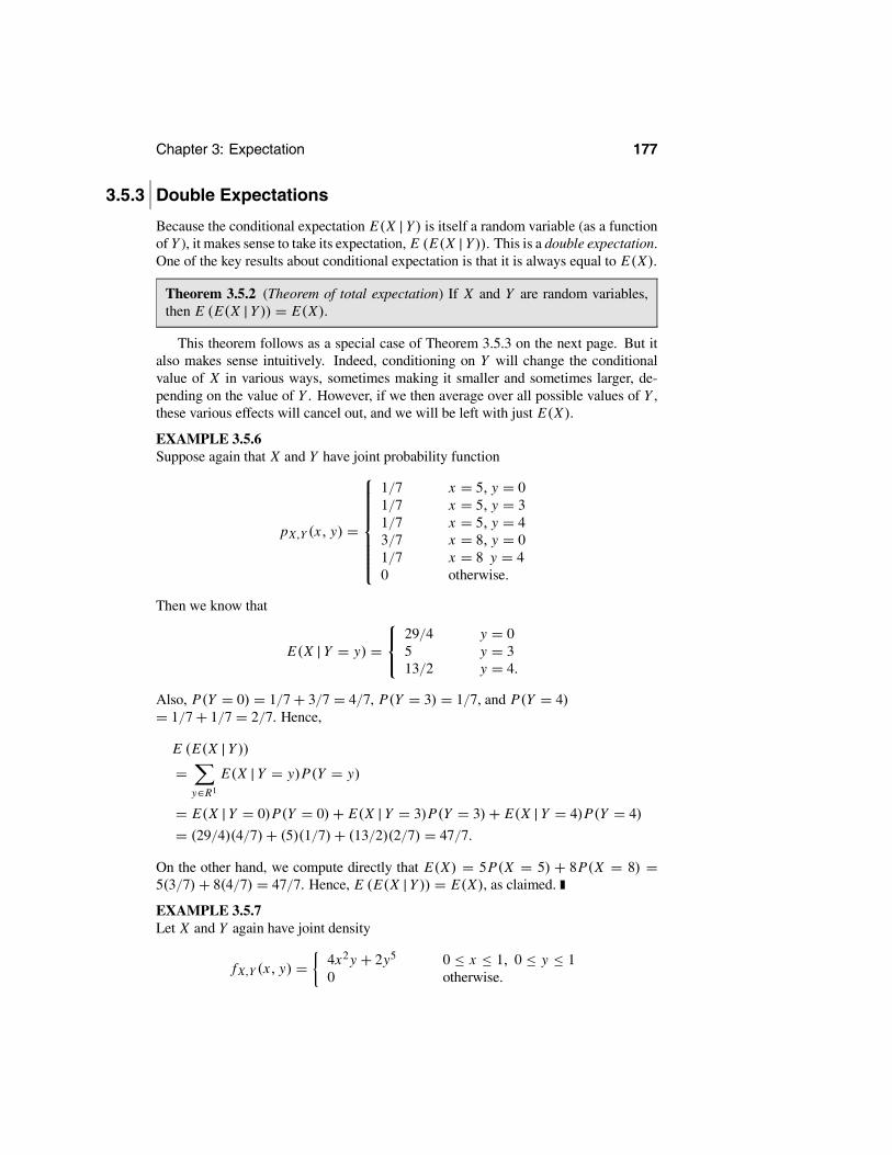
Chapter 3: Expectation 177
3.5.3 Double Expectations
Because the conditional expectation E(X |Y ) is itself a random variable (as a functionof Y ), it makes sense to take its expectation, E (E(X |Y )). This is a double expectation.One of the key results about conditional expectation is that it is always equal to E(X).
Theorem 3.5.2 (Theorem of total expectation) If X and Y are random variables,then E (E(X |Y )) = E(X).
This theorem follows as a special case of Theorem 3.5.3 on the next page. But italso makes sense intuitively. Indeed, conditioning on Y will change the conditionalvalue of X in various ways, sometimes making it smaller and sometimes larger, de-pending on the value of Y . However, if we then average over all possible values of Y ,these various effects will cancel out, and we will be left with just E(X).
EXAMPLE 3.5.6Suppose again that X and Y have joint probability function
pX,Y (x, y) =
1/7 x = 5, y = 01/7 x = 5, y = 31/7 x = 5, y = 43/7 x = 8, y = 01/7 x = 8 y = 40 otherwise.
Then we know that
E(X |Y = y) = 29/4 y = 0
5 y = 313/2 y = 4.
Also, P(Y = 0) = 1/7+ 3/7 = 4/7, P(Y = 3) = 1/7, and P(Y = 4)= 1/7+ 1/7 = 2/7. Hence,
E (E(X |Y ))=
y∈R1
E(X |Y = y)P(Y = y)
= E(X |Y = 0)P(Y = 0)+ E(X |Y = 3)P(Y = 3)+ E(X |Y = 4)P(Y = 4)
= (29/4)(4/7)+ (5)(1/7)+ (13/2)(2/7) = 47/7.
On the other hand, we compute directly that E(X) = 5P(X = 5) + 8P(X = 8) =5(3/7)+ 8(4/7) = 47/7. Hence, E (E(X |Y )) = E(X), as claimed.
EXAMPLE 3.5.7Let X and Y again have joint density
fX,Y (x, y) = 4x2y + 2y5 0 ≤ x ≤ 1, 0 ≤ y ≤ 10 otherwise.

178 Section 3.5: Conditional Expectation
We already know that
E(X |Y ) = 1+ Y 4 / 4/3+ 2Y 4
and that fY (y) = 4y/3+ 2y5 for 0 ≤ y ≤ 1. Hence,
E (E(X |Y ))= E
1+ Y 4
4/3+ 2Y 4 =∞
−∞E(X |Y = y) fY (y) dy
=1
0
1+ y4
4/3+ 2y4 (4y/3+ 2y5) dy =1
0(y + y5) dy = 1/2+ 1/6 = 2/3.
On the other hand,
E(X) =∞
−∞
∞
−∞x fX,Y (x, y) dy dx =
1
0
1
0x (4x2y + 2y5) dy dx
=1
0x (2x2 + 2/6) dx =
1
0(2x3 + x/3) dx = 2/4+ 1/6 = 2/3 .
Hence, E (E(X |Y )) = E(X), as claimed.
Theorem 3.5.2 is a special case (with g(y) ≡ 1) of the following more generalresult, which in fact characterizes conditional expectation.
Theorem 3.5.3 Let X and Y be random variables, and let g : R1 → R1 be anyfunction. Then E(g(Y )E(X |Y )) = E(g(Y )X).
PROOF See Section 3.8 for the proof of this result.
We also note the following related result. It says that, when conditioning on Y , anyfunction of Y can be factored out since it is effectively a constant.
Theorem 3.5.4 Let X and Y be random variables, and let g : R1 → R1 be anyfunction. Then E(g(Y )X |Y ) = g(Y )E(X |Y ).
PROOF See Section 3.8 for the proof of this result.
Finally, because conditioning twice on Y is the same as conditioning just once onY , we immediately have the following.
Theorem 3.5.5 Let X and Y be random variables. Then E(E(X |Y )|Y ) = E(X |Y ).
3.5.4 Conditional Variance (Advanced)
In addition to defining conditional expectation, we can define conditional variance. Asusual, this involves the expected squared distance of a random variable to its mean.
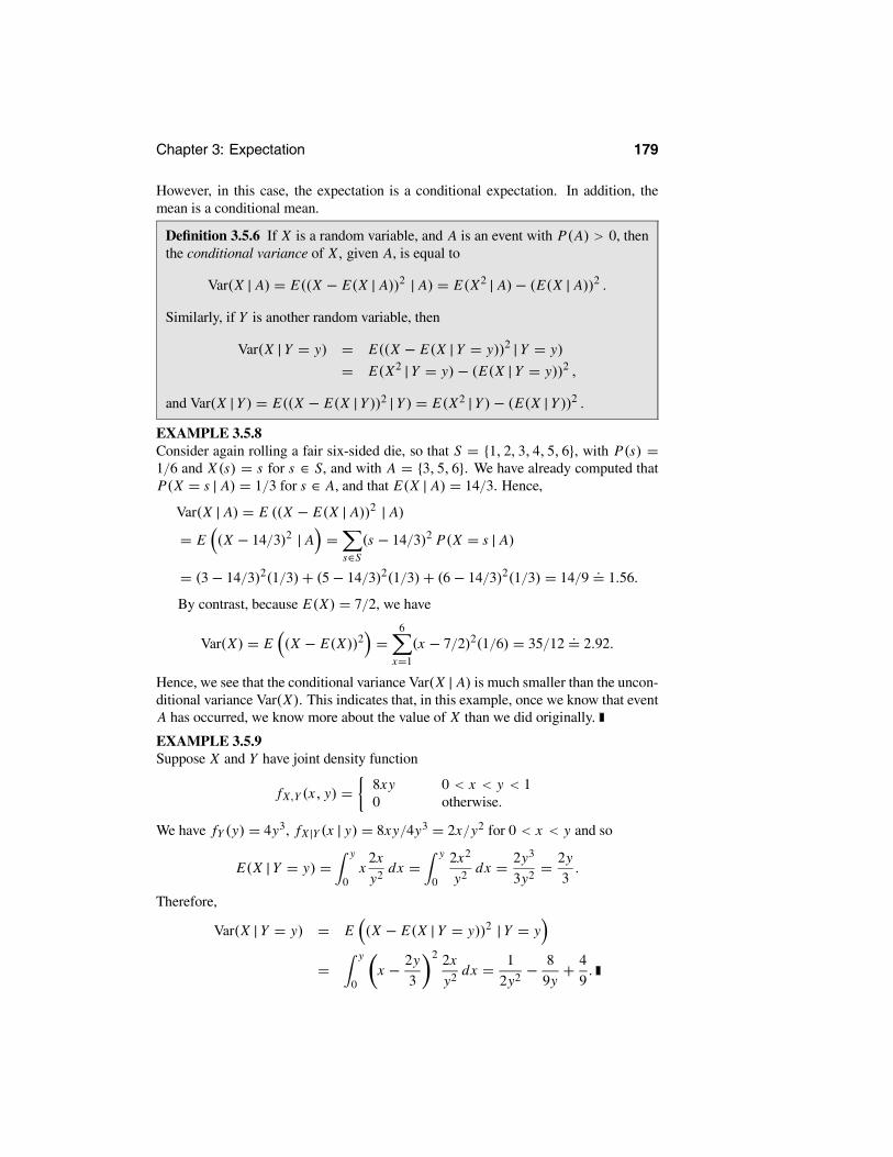
Chapter 3: Expectation 179
However, in this case, the expectation is a conditional expectation. In addition, themean is a conditional mean.
Definition 3.5.6 If X is a random variable, and A is an event with P(A) > 0, thenthe conditional variance of X, given A, is equal to
Var(X | A) = E((X − E(X | A))2 | A) = E(X2 | A)− (E(X | A))2 .Similarly, if Y is another random variable, then
Var(X |Y = y) = E((X − E(X |Y = y))2 |Y = y)
= E(X2 |Y = y)− (E(X |Y = y))2 ,
and Var(X |Y ) = E((X − E(X |Y ))2 |Y ) = E(X2 |Y )− (E(X |Y ))2 .EXAMPLE 3.5.8Consider again rolling a fair six-sided die, so that S = {1, 2, 3, 4, 5, 6}, with P(s) =1/6 and X (s) = s for s ∈ S, and with A = {3, 5, 6}. We have already computed thatP(X = s | A) = 1/3 for s ∈ A, and that E(X | A) = 14/3. Hence,
Var(X | A) = E ((X − E(X | A))2 | A)= E (X − 14/3)2 | A =
s∈S
(s − 14/3)2 P(X = s | A)
= (3− 14/3)2(1/3)+ (5− 14/3)2(1/3)+ (6− 14/3)2(1/3) = 14/9.= 1.56.
By contrast, because E(X) = 7/2, we have
Var(X) = E (X − E(X))2 =6
x=1
(x − 7/2)2(1/6) = 35/12.= 2.92.
Hence, we see that the conditional variance Var(X | A) is much smaller than the uncon-ditional variance Var(X). This indicates that, in this example, once we know that eventA has occurred, we know more about the value of X than we did originally.
EXAMPLE 3.5.9Suppose X and Y have joint density function
fX,Y (x, y) = 8xy 0 < x < y < 10 otherwise.
We have fY (y) = 4y3, fX |Y (x | y) = 8xy/4y3 = 2x/y2 for 0 < x < y and so
E(X |Y = y) =y
0x
2x
y2dx =
y
0
2x2
y2dx = 2y3
3y2= 2y
3.
Therefore,
Var(X |Y = y) = E (X − E(X |Y = y))2 |Y = y
=y
0x − 2y
3
2 2x
y2dx = 1
2y2− 8
9y+ 4
9.

180 Section 3.5: Conditional Expectation
Finally, we note that conditional expectation and conditional variance satisfy thefollowing useful identity.
Theorem 3.5.6 For random variables X and Y ,
Var(X) = Var (E(X |Y ))+ E (Var(X |Y )) .
PROOF See Section 3.8 for the proof of this result.
Summary of Section 3.5
• If X is discrete, then the conditional expectation of X, given an event A, is equalto E(X | A) = x∈R1 x P(X = x | A).
• If X and Y are discrete random variables, then E(X |Y ) is itself a random vari-able, with E(X |Y ) equal to E(X |Y = y) when Y = y.
• If X and Y are jointly absolutely continuous, then E(X |Y ) is itself a randomvariable, with E(X |Y ) equal to E(X |Y = y) when Y = y, where E(X |Y =y) = x fX |Y (x | y) dx .
• Conditional expectation is linear.
• We always have that E (g(Y ) E(X |Y )) = E (g(Y ) X), and E (E(X |Y )|Y ) =E(X |Y ).
• Conditional variance is given by Var(X |Y ) = E(X2 |Y )− (E(X |Y ))2.
EXERCISES
3.5.1 Suppose X and Y are discrete, with
pX,Y (x, y) =
1/5 x = 2, y = 31/5 x = 3, y = 21/5 x = 3, y = 31/5 x = 2, y = 21/5 x = 3, y = 170 otherwise.
(a) Compute E(X |Y = 3).(b) Compute E(Y | X = 3).(c) Compute E(X |Y ).(d) Compute E(Y | X).3.5.2 Suppose X and Y are jointly absolutely continuous, with
fX,Y (x, y) = 9(xy + x5y5)/16, 000, 900 0 ≤ x ≤ 4, 0 ≤ y ≤ 50 otherwise.
(a) Compute fX (x).

Chapter 3: Expectation 181
(b) Compute fY (y).(c) Compute E(X |Y ).(d) Compute E(Y | X).(e) Compute E (E(X |Y )), and verify that it is equal to E(X).3.5.3 Suppose X and Y are discrete, with
pX,Y (x, y) =
1/11 x = −4, y = 22/11 x = −4, y = 34/11 x = −4, y = 71/11 x = 6, y = 21/11 x = 6, y = 31/11 x = 6, y = 71/11 x = 6, y = 130 otherwise.
(a) Compute E(Y | X = 6).(b) Compute E(Y | X = −4).(c) Compute E(Y | X).3.5.4 Let pX,Y be as in the previous exercise.(a) Compute E(X |Y = 2).(b) Compute E(X |Y = 3).(c) Compute E(X |Y = 7).(d) Compute E(X |Y = 13).(e) Compute E(X |Y ).3.5.5 Suppose that a student must choose one of two summer job offers. If it is not nec-essary to take a summer course, then a job as a waiter will produce earnings (roundedto the nearest $1000) with the following probability distribution.
$1000 $2000 $3000 $40000.1 0.3 0.4 0.2
If it is necessary to take a summer course, then a part-time job at a hotel will produceearnings (rounded to the nearest $1000) with the following probability distribution.
$1000 $2000 $3000 $40000.3 0.4 0.2 0.1
If the probability that the student will have to take the summer course is 0.6, thendetermine the student’s expected summer earnings.3.5.6 Suppose you roll two fair six-sided dice. Let X be the number showing on thefirst die, and let Z be the sum of the two numbers showing.(a) Compute E(X).(b) Compute E(Z | X = 1).(c) Compute E(Z | X = 6).(d) Compute E(X | Z = 2).(e) Compute E(X | Z = 4).

182 Section 3.5: Conditional Expectation
(f) Compute E(X | Z = 6).(g) Compute E(X | Z = 7).(h) Compute E(X | Z = 11).3.5.7 Suppose you roll two fair six-sided dice. Let Z be the sum of the two numbersshowing, and let W be the product of the two numbers showing.(a) Compute E(Z |W = 4).(b) Compute E(W | Z = 4).3.5.8 Suppose you roll one fair six-sided die and then flip as many coins as the numbershowing on the die. (For example, if the die shows 4, then you flip four coins.) Let Xbe the number showing on the die, and Y be the number of heads obtained.(a) Compute E(Y | X = 5).(b) Compute E(X |Y = 0).(c) Compute E(X |Y = 2).3.5.9 Suppose you flip three fair coins. Let X be the number of heads obtained, andlet Y = 1 if the first coin shows heads, otherwise Y = 0.(a) Compute E(X |Y = 0).(b) Compute E(X |Y = 1).(c) Compute E(Y | X = 0).(d) Compute E(Y | X = 1).(e) Compute E(Y | X = 2).(f) Compute E(Y | X = 3).(g) Compute E(Y | X).(h) Verify directly that E[E(Y | X)] = E(Y ).3.5.10 Suppose you flip one fair coin and roll one fair six-sided die. Let X be thenumber showing on the die, and let Y = 1 if the coin is heads with Y = 0 if the coin istails. Let Z = XY .(a) Compute E(Z).(b) Compute E(Z | X = 4).(c) Compute E(Y | X = 4).(d) Compute E(Y | Z = 4).(e) Compute E(X | Z = 4).3.5.11 Suppose X and Y are jointly absolutely continuous, with joint density functionfX,Y (x, y) = (6/19)(x2 + y3) for 0 < x < 2 and 0 < y < 1, otherwise fX,Y (x, y) =0.(a) Compute E(X).(b) Compute E(Y ).(c) Compute E(X |Y ).(d) Compute E(Y | X).(e) Verify directly that E[E(X |Y )] = E(X).(f) Verify directly that E[E(Y | X)] = E(Y ).
PROBLEMS
3.5.12 Suppose there are two urns. Urn I contains 100 chips: 30 are labelled 1, 40are labelled 2, and 30 are labelled 3. Urn 2 contains 100 chips: 20 are labelled 1,

Chapter 3: Expectation 183
50 are labelled 2, and 30 are labelled 3. A coin is tossed and if a head is observed,then a chip is randomly drawn from urn 1, otherwise a chip is randomly drawn fromurn 2. The value Y on the chip is recorded. If an occurrence of a head on the coinis denoted by X = 1, a tail by X = 0, and X ∼ Bernoulli(3/4) , then determineE(X |Y ), E(Y | X), E(Y ), and E(X).
3.5.13 Suppose that five coins are each tossed until the first head is obtained on eachcoin and where each coin has probability θ of producing a head. If you are told that thetotal number of tails observed is Y = 10, then determine the expected number of tailsobserved on the first coin.3.5.14 (Simpson’s paradox) Suppose that the conditional distributions of Y, given X,are shown in the following table. For example, pY |X (1 | i) could correspond to theprobability that a randomly selected heart patient at hospital i has a successful treat-ment.
pY |X (0 | 1) pY |X (1 | 1)0.030 0.970
pY |X (0 | 2) pY |X (1 | 2)0.020 0.980
(a) Compute E(Y | X).(b) Now suppose that patients are additionally classified as being seriously ill (Z = 1),or not seriously ill (Z = 0). The conditional distributions of Y, given (X, Z), areshown in the following tables. Compute E(Y | X, Z).
pY |X,Z (0 | 1, 0) pY |X,Z (1 | 1, 0)0.010 0.990
pY |X,Z (0 | 2, 0) pY |X,Z (1 | 2, 0)0.013 0.987
pY |X,Z (0 | 1, 1) pY |X,Z (1 | 1, 1)0.038 0.962
pY |X,Z (0 | 2, 1) pY |X,Z (1 | 2, 1)0.040 0.960
(c) Explain why the conditional distributions in part (a) indicate that hospital 2 is thebetter hospital for a patient who needs to undergo this treatment, but all the conditionaldistributions in part (b) indicate that hospital 1 is the better hospital. This phenomenonis known as Simpson’s paradox.(d) Prove that, in general, pY |X (y | x) = z pY |X,Z (y | x, z) pZ |X (z | x) and E(Y | X)= E(E(Y | X, Z) | X).(e) If the conditional distributions pZ |X (· | x) , corresponding to the example discussedin parts (a) through (c) are given in the following table, verify the result in part (d)numerically and explain how this resolves Simpson’s paradox.
pZ |X (0 | 1) pZ |X (1 | 1)0.286 0.714
pZ |X (0 | 2) pZ |X (1 | 2)0.750 0.250

184 Section 3.6: Inequalities
3.5.15 Present an example of a random variable X , and an event A with P(A) > 0,such that Var(X | A) >Var(X). (Hint: Suppose S = {1, 2, 3} with X (s) = s, andA = {1, 3}.)3.5.16 Suppose that X , given Y = y, is distributed Gamma(α, y) and that the marginaldistribution of Y is given by 1/Y ∼ Exponential(λ) . Determine E (X) .
3.5.17 Suppose that (X,Y ) ∼Bivariate Normal (µ1, µ2, σ 1, σ 2, ρ). Use (2.7.1) (whengiven Y = y) and its analog (when given X = x) to determine E(X |Y ), E(Y | X),Var(X |Y ), and Var(Y | X).3.5.18 Suppose that (X1, X2, X3) ∼Multinomial(n, θ1, θ2, θ3). Determine E(X1 | X2)and Var(X1 | X2). (Hint: Show that X1, given X2 = x2, has a binomial distribution.)3.5.19 Suppose that (X1, X2) ∼ Dirichlet(α1, α2, α3). Determine E(X1 | X2) andVar(X1 | X2). (Hint: First show that X1/(1 − x2), given X2 = x2, has a beta dis-tribution and then use Problem 3.3.24.)3.5.20 Let fX,Y be as in Exercise 3.5.2.(a) Compute Var(X).(b) Compute Var(E(X |Y )).(c) Compute Var(X |Y ).(d) Verify that Var(X) =Var(E(X |Y ))+ E (Var(X |Y )).3.5.21 Suppose we have three discrete random variables X, Y, and Z . We say that Xand Y are conditionally independent, given Z, if
pX,Y |Z (x, y | z) = pX |Z (x | z) pY |Z (y | z)for every x, y, and z such that P (Z = z) > 0. Prove that when X and Y are condition-ally independent, given Z, then
E (g(X)h(Y ) | Z) = E (g(X) | Z) E (h(Y ) | Z) .
3.6 InequalitiesExpectation and variance are closely related to the underlying distributions of randomvariables. This relationship allows us to prove certain inequalities that are often veryuseful. We begin with a classic result, Markov’s inequality, which is very simple butalso very useful and powerful.
Theorem 3.6.1 (Markov’s inequality) If X is a nonnegative random variable, thenfor all a > 0,
P(X ≥ a) ≤ E(X)
a.
That is, the probability that X exceeds any given value a is no more than the meanof X divided by a.
PROOF Define a new random variable Z by
Z = a X ≥ a0 X < a.

Chapter 3: Expectation 185
Then clearly Z ≤ X , so that E(Z) ≤ E(X) by monotonicity. On the other hand,
E(Z) = a P(Z = a)+ 0 P(Z = 0) = a P(Z = a) = a P(X ≥ a).
So, E(X) ≥ E(Z) = a P(X ≥ a). Rearranging, P(X ≥ a) ≤ E(X)/a, as claimed.
Intuitively, Markov’s inequality says that if the expected value of X is small, thenit is unlikely that X will be too large. We now consider some applications of Theorem3.6.1.
EXAMPLE 3.6.1Suppose P(X = 3) = 1/2, P(X = 4) = 1/3, and P(X = 7) = 1/6. Then E(X) =3(1/2) + 4(1/3) + 7(1/6) = 4. Hence, setting a = 6, Markov’s inequality says thatP(X ≥ 6) ≤ 4/6 = 2/3. In fact, P(X ≥ 6) = 1/6 < 2/3.
EXAMPLE 3.6.2Suppose P(X = 2) = P(X = 8) = 1/2. Then E(X) = 2(1/2) + 8(1/2) = 5.Hence, setting a = 8, Markov’s inequality says that P(X ≥ 8) ≤ 5/8. In fact,P(X ≥ 8) = 1/2 < 5/8.
EXAMPLE 3.6.3Suppose P(X = 0) = P(X = 2) = 1/2. Then E(X) = 0(1/2) + 2(1/2) = 1.Hence, setting a = 2, Markov’s inequality says that P(X ≥ 2) ≤ 1/2. In fact,P(X ≥ 2) = 1/2, so Markov’s inequality is an equality in this case.
Markov’s inequality is also used to prove Chebychev’s inequality, perhaps the mostimportant inequality in all of probability theory.
Theorem 3.6.2 (Chebychev’s inequality) Let Y be an arbitrary random variable,with finite mean µY . Then for all a > 0,
P (|Y − µY | ≥ a) ≤ Var(Y )a2 .
PROOF Set X = (Y−µY )2. Then X is a nonnegative random variable. Thus, using
Theorem 3.6.1, we have P (|Y − µY | ≥ a) = P X ≥ a2 ≤ E(X)/a2 =Var(Y )/a2,and this establishes the result.
Intuitively, Chebychev’s inequality says that if the variance of Y is small, then itis unlikely that Y will be too far from its mean value µY . We now consider someexamples.
EXAMPLE 3.6.4Suppose again that P(X = 3) = 1/2, P(X = 4) = 1/3, and P(X = 7) = 1/6.Then E(X) = 4, as above. Also, E(X2) = 9(1/2) + 16(1/3) + 49(1/6) = 18, sothat Var(X) = 18 − 42 = 2. Hence, setting a = 1, Chebychev’s inequality saysthat P(|X − 4| ≥ 1) ≤ 2/12 = 2, which tells us nothing because we always haveP(|X − 4| ≥ 1) ≤ 1. On the other hand, setting a = 3, we get P(|X − 4| ≥ 3) ≤2/32 = 2/9, which is true because in fact P(|X − 4| ≥ 3) = P(X = 7) = 1/6 < 2/9.

186 Section 3.6: Inequalities
EXAMPLE 3.6.5Let X ∼ Exponential(3), and let a = 5. Then E(X) = 1/3 and Var(X) = 1/9. Hence,by Chebychev’s inequality with a = 1/2, P(|X−1/3| ≥ 1/2) ≤ (1/9)/(1/2)2 = 4/9.On the other hand, because X ≥ 0, P(|X − 1/3| ≥ 1/2) = P(X ≥ 5/6), andby Markov’s inequality, P(X ≥ 5/6) ≤ (1/3)/(5/6) = 2/5. Because 2/5 < 4/9, weactually get a better bound from Markov’s inequality than from Chebychev’s inequalityin this case.
EXAMPLE 3.6.6Let Z ∼ N(0, 1), and a = 5. Then by Chebychev’s inequality, P(|Z | ≥ 5) ≤ 1/5.
EXAMPLE 3.6.7Let X be a random variable having very small variance. Then Chebychev’s inequalitysays that P(|X−µX | ≥ a) is small whenever a is not too small. In other words, usually|X − µX | is very small, i.e., X ≈ µX . This makes sense, because if the variance of Xis very small, then usually X is very close to its mean value µX .
Inequalities are also useful for covariances, as follows.
Theorem 3.6.3 (Cauchy–Schwartz inequality) Let X and Y be arbitrary randomvariables, each having finite, nonzero variance. Then
|Cov(X, Y )| ≤ Var(X)Var(Y ).
Furthermore, if Var(Y ) > 0, then equality is attained if and only if X − µX =λ(Y − µY ) where λ =Cov(X,Y )/Var(Y ).
PROOF See Section 3.8 for the proof.
The Cauchy–Schwartz inequality says that if the variance of X or Y is small, thenthe covariance of X and Y must also be small.
EXAMPLE 3.6.8Suppose X = C is a constant. Then Var(X) = 0. It follows from the Cauchy–Schwartz inequality that, for any random variable Y , we must have Cov(X,Y ) ≤(Var(X)Var(Y ))1/2 = (0 Var(Y ))1/2 = 0, so that Cov(X,Y ) = 0.
Recalling that the correlation of X and Y is defined by
Corr(X,Y ) = Cov(X,Y )√Var(X)Var(Y )
,
we immediately obtain the following important result (which has already been referredto, back when correlation was first introduced).
Corollary 3.6.1 Let X and Y be arbitrary random variables, having finite meansand finite, nonzero variances. Then |Corr(X, Y )| ≤ 1. Furthermore, |Corr(X, Y )| =1 if and only if
X − µX = Cov(X, Y )Var (Y )
(Y − µY ).

Chapter 3: Expectation 187
So the correlation between two random variables is always between −1 and 1. Wealso see that X and Y are linearly related if and only if |Corr(X, Y )| = 1, and thatthis relationship is increasing (positive slope) when Corr(X,Y ) = 1 and decreasing(negative slope) when Corr(X, Y ) = −1.
3.6.1 Jensen’s Inequality (Advanced)
Finally, we develop a more advanced inequality that is sometimes very useful. A func-tion f is called convex if for every x < y, the line segment from (x, f (x)) to (y, f (y))lies entirely above the graph of f, as depicted in Figure 3.6.1.
2.0 2.5 3.0 3.5 4.0 4.5 5.0
100
200
300
400
500
600
x
f
Figure 3.6.1: Plot of the convex function f (x) = x4 and the line segment joining (2, f (2)) to(4, f (4)).
In symbols, we require that for every x < y and every 0 < λ < 1, we haveλ f (x) + (1 − λ) f (y) ≥ f (λx + (1 − λ)y). Examples of convex functions includef (x) = x2, f (x) = x4, and f (x) = max(x,C) for any real number C . We have thefollowing.
Theorem 3.6.4 (Jensen’s inequality) Let X be an arbitrary random variable, and letf : R1 → R1 be a convex function such that E( f (X)) is finite. Then f (E(X)) ≤E( f (X)). Equality occurs if and only if f (X) = a + bX for some a and b.
PROOF Because f is convex, we can find a linear function g(x) = ax + b suchthat g(E(X)) = f (E(X)) and g(x) ≤ f (x) for all x ∈ R1 (see, for example, Figure3.6.2).

188 Section 3.6: Inequalities
2.2 2.4 2.6 2.8 3.0 3.2 3.4 3.6 3.8 4.00
50
100
150
200
250
x
f
Figure 3.6.2: Plot of the convex function f (x) = x4 and the functiong(x) = 81+ 108(x − 3), satisfying g(x) ≤ f (x) on the interval (2, 4) .
But then using monotonicity and linearity, we have E( f (X)) ≥ E(g(X)) =E(aX + b) = aE(X)+ b = g(E(X)) = f (E(X)), as claimed.
We have equality if and only if 0 = E( f (X)− g(X)). Because f (X)− g(X) ≥ 0,this occurs (using Challenge 3.3.29) if and only if f (X) = g(X) = aX + b withprobability 1.
EXAMPLE 3.6.9Let X be a random variable with finite variance. Then setting f (x) = x2, Jensen’sinequality says that E(X2) ≥ (E(X))2. Of course, we already knew this becauseE(X2)− (E(X))2 =Var(X) ≥ 0.
EXAMPLE 3.6.10Let X be a random variable with finite fourth moment. Then setting f (x) = x4,Jensen’s inequality says that E(X4) ≥ (E(X))4.
EXAMPLE 3.6.11Let X be a random variable with finite mean, and let M ∈ R1. Then setting f (x) =max(x,M), we have that E(max(X,M)) ≥ max(E(X),M) by Jensen’s inequality. Infact, we could also have deduced this from the monotonicity property of expectation,using the two inequalities max(X,M) ≥ X and max(X,M) ≥ M.
Summary of Section 3.6
• For nonnegative X,Markov’s inequality says P(X ≥ a) ≤ E(X)/a.
• Chebychev’s inequality says P(|Y − µY | ≥ a) ≤Var(Y )/a2.
• The Cauchy–Schwartz inequality says |Cov(X, Y )| ≤ (Var(X)Var(Y ))1/2, sothat |Corr(X, Y )| ≤ 1.

Chapter 3: Expectation 189
• Jensen’s inequality says f (E(X)) ≤ E( f (X)) whenever f is convex.
EXERCISES
3.6.1 Let Z ∼ Poisson(3). Use Markov’s inequality to get an upper bound on P(Z ≥7).3.6.2 Let X ∼ Exponential(5). Use Markov’s inequality to get an upper bound onP(X ≥ 3) and compare it with the precise value.3.6.3 Let X ∼ Geometric(1/2).(a) Use Markov’s inequality to get an upper bound on P(X ≥ 9).(b) Use Markov’s inequality to get an upper bound on P(X ≥ 2).(c) Use Chebychev’s inequality to get an upper bound on P(|X − 1| ≥ 1).(d) Compare the answers obtained in parts (b) and (c).3.6.4 Let Z ∼ N(5, 9). Use Chebychev’s inequality to get an upper bound on P(|Z −5| ≥ 30).3.6.5 Let W ∼ Binomial(100, 1/2), as in the number of heads when flipping 100 faircoins. Use Chebychev’s inequality to get an upper bound on P(|W − 50| ≥ 10).3.6.6 Let Y ∼ N(0, 100), and let Z ∼ Binomial(80, 1/4). Determine (with explana-tion) the largest and smallest possible values of Cov(Y, Z).3.6.7 Let X ∼ Geometric(1/11). Use Jensen’s inequality to determine a lower boundon E(X4), in two different ways.(a) Apply Jensen’s inequality to X with f (x) = x4.(b) Apply Jensen’s inequality to X2 with f (x) = x2.3.6.8 Let X be the number showing on a fair six-sided die. What bound does Cheby-chev’s inequality give for P(X ≥ 5 or X ≤ 2)?3.6.9 Suppose you flip four fair coins. Let Y be the number of heads obtained.(a) What bound does Chebychev’s inequality give for P(Y ≥ 3 or Y ≤ 1)?(b) What bound does Chebychev’s inequality give for P(Y ≥ 4 or Y ≤ 0)?3.6.10 Suppose W has density function f (w) = 3w2 for 0 < w < 1, otherwisef (w) = 0.(a) Compute E(W).(b) What bound does Chebychev’s inequality give for P(|W − E(W )| ≥ 1/4)?3.6.11 Suppose Z has density function f (z) = z3/4 for 0 < z < 2, otherwise f (z) =0.(a) Compute E(Z).(b) What bound does Chebychev’s inequality give for P(|Z − E(Z)| ≥ 1/2)?3.6.12 Suppose Var(X) = 4 and Var(Y ) = 9.(a) What is the largest possible value of Cov(X, Y )?(b) What is the smallest possible value of Cov(X,Y )?(c) Suppose Z = 3X/2. Compute Var(Z) and Cov(X, Z), and compare your answerwith part (a).(d) Suppose W = −3X/2. Compute Var(W ) and Cov(W, Z), and compare your an-swer with part (b).

190 Section 3.6: Inequalities
3.6.13 Suppose a species of beetle has length 35 millimeters on average. Find an upperbound on the probability that a randomly chosen beetle of this species will be over 80millimeters long.
PROBLEMS
3.6.14 Prove that for any > 0 and δ > 0, there is a positive integer M, such that if Xis the number of heads when flipping M fair coins, then P(|(X/M)− (1/2)| ≥ δ) ≤ .3.6.15 Prove that for any µ and σ 2 > 0, there is a > 0 and a random variable X withE(X) = µ and Var(X) = σ 2, such that Chebychev’s inequality holds with equality,i.e., such that P(|X − µ| ≥ a) = σ 2/a2.3.6.16 Suppose that (X,Y ) is uniform on the set {(x1, y1) , . . . , (xn, yn)} where thex1, . . . , xn are distinct values and the y1, . . . , yn are distinct values.(a) Prove that X is uniformly distributed on x1, . . . , xn, with mean given by x =n−1 n
i=1 xi and variance given by s2X = n−1 n
i=1 (xi − x)2 .
(b) Prove that the correlation coefficient between X and Y is given by
rXY =ni=1 (xi − x) (yi − y)
ni=1 (xi − x)2 n
i=1 (yi − y)2= sXY
sX sY
where sXY = n−1 ni=1 (xi − x) (yi − y) . The value sXY is referred to as the sample
covariance and rXY is referred to as the sample correlation coefficient when the values(x1, y1) , . . . , (xn, yn) are an observed sample from some bivariate distribution.(c) Argue that rXY is also the correlation coefficient between X and Y when we dropthe assumption of distinctness for the xi and yi .(d) Prove that −1 ≤ rXY ≤ 1 and state the conditions under which rXY = ±1.3.6.17 Suppose that X is uniformly distributed on {x1, . . . , xn} and so has mean x =n−1 n
i=1 xi and variance s2X = n−1 n
i=1 (xi − x)2 (see Problem 3.6.16(a)). What isthe largest proportion of the values xi that can lie outside x − 2sX , x + 2sX ?
3.6.18 Suppose that X is distributed with density given by fX (x) = 2/x3 for x > 1and is 0 otherwise.(a) Prove that fX is a density.(b) Calculate the mean of X.
(c) Compute P(X ≥ k) and compare this with the upper bound on this quantity givenby Markov’s inequality.(d) What does Chebyshev’s inequality say in this case?3.6.19 Let g(x) = max(−x,−10).(a) Verify that g is a convex function.(b) Suppose Z ∼ Exponential(5). Use Jensen’s inequality to obtain a lower bound onE(g(Z)).3.6.20 It can be shown that a function f, with continuous second derivative, is convexon (a, b) if f (x) > 0 for all x ∈ (a, b) .(a) Use the above fact to show that f (x) = x p is convex on (0,∞) whenever p ≥ 1.
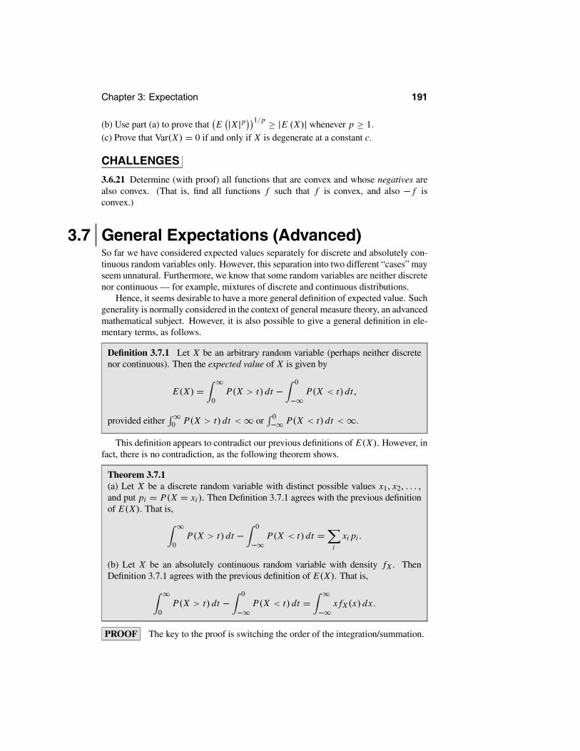
Chapter 3: Expectation 191
(b) Use part (a) to prove that E |X |p 1/p ≥ |E (X)| whenever p ≥ 1.(c) Prove that Var(X) = 0 if and only if X is degenerate at a constant c.
CHALLENGES
3.6.21 Determine (with proof) all functions that are convex and whose negatives arealso convex. (That is, find all functions f such that f is convex, and also − f isconvex.)
3.7 General Expectations (Advanced)So far we have considered expected values separately for discrete and absolutely con-tinuous random variables only. However, this separation into two different “cases” mayseem unnatural. Furthermore, we know that some random variables are neither discretenor continuous — for example, mixtures of discrete and continuous distributions.
Hence, it seems desirable to have a more general definition of expected value. Suchgenerality is normally considered in the context of general measure theory, an advancedmathematical subject. However, it is also possible to give a general definition in ele-mentary terms, as follows.
Definition 3.7.1 Let X be an arbitrary random variable (perhaps neither discretenor continuous). Then the expected value of X is given by
E(X) =∞
0P(X > t) dt −
0
−∞P(X < t) dt,
provided either ∞0 P(X > t) dt <∞ or 0
−∞ P(X < t) dt <∞.
This definition appears to contradict our previous definitions of E(X). However, infact, there is no contradiction, as the following theorem shows.
Theorem 3.7.1(a) Let X be a discrete random variable with distinct possible values x1, x2, . . . ,and put pi = P(X = xi). Then Definition 3.7.1 agrees with the previous definitionof E(X). That is,
∞
0P(X > t) dt −
0
−∞P(X < t) dt =
i
xi pi .
(b) Let X be an absolutely continuous random variable with density fX . ThenDefinition 3.7.1 agrees with the previous definition of E(X). That is,
∞
0P(X > t) dt −
0
−∞P(X < t) dt =
∞
−∞x fX (x) dx.
PROOF The key to the proof is switching the order of the integration/summation.

192 Section 3.7: General Expectations (Advanced)
(a) We have
∞
0P(X > t) dt =
∞
0 i,xi>t
pi dt =i
pi
xi
0dt =
i
pi xi ,
as claimed.
(b) We have
∞
0P(X > t) dt =
∞
0
∞
tfX (x) dx dt =
∞
0
x
0fX (x) dt dx
=∞
0x fX (x) dx .
Similarly,
0
−∞P(X < t) dt =
0
−∞
t
−∞fX (x) dx dt =
0
−∞
0
xfX (x) dt dx
=0
−∞(−x) fX (x) dx.
Hence,
∞
0P(X > t) dt −
0
−∞P(X < t) dt =
∞
0x fX (x) dx −
0
−∞(−x) fX (x) dx
=∞
−∞x fX (x) dx,
as claimed.
In other words, Theorem 3.7.1 says that Definition 3.7.1 includes our previous defi-nitions of expected value, for both discrete and absolutely continuous random variables,while working for any random variable at all. (Note that to apply Definition 3.7.1 wetake an integral, not a sum, regardless of whether X is discrete or continuous!)
Furthermore, Definition 3.7.1 preserves the key properties of expected value, asthe following theorem shows. (We omit the proof here, but see Challenge 3.7.10 for aproof of part (c).)
Theorem 3.7.2 Let X and Y be arbitrary random variables, perhaps neither discretenor continuous, with expected values defined by Definition 3.7.1.(a) (Linearity) If a and b are any real numbers, then E(aX+bY ) = aE(X)+bE(Y ).(b) If X and Y are independent, then E(XY ) = E(X) E(Y ).(c) (Monotonicity) If X ≤ Y , then E(X) ≤ E(Y ).
Definition 3.7.1 also tells us about expected values of mixture distributions, as fol-lows.

Chapter 3: Expectation 193
Theorem 3.7.3 For 1 ≤ i ≤ k, let Yi be a random variable with cdf Fi . Let X bea random variable whose cdf corresponds to a finite mixture (as in Section 2.5.4)of the cdfs of the Yi , so that FX (x) = i pi Fi (x), where pi ≥ 0 and i pi = 1.Then E(X) = i pi E(Yi ).
PROOF We compute that
P(X > t) = 1− FX (t) = 1−i
pi Fi (t)
=i
pi (1− Fi(t)) =i
pi P(Yi > t).
Similarly,
P(X < t) = FX (t−) =
i
pi Fi (t−) =
i
pi P(Yi < t).
Hence, from Definition 3.7.1,
E(X) =∞
0P(X > t) dt −
0
−∞P(X < t) dt
=∞
0 i
pi P(Yi > t) dt −0
−∞ i
pi P(Yi < t) dt
=i
pi
∞
0P(Yi > t) dt −
0
−∞P(Yi < t) dt
=i
pi E(Yi ),
as claimed.
Summary of Section 3.7
• For general random variables, we can define a general expected value by E(X) =∞0 P(X > t) dt − 0
−∞ P(X < t) dt .
• This definition agrees with our previous one, for discrete or absolutely continu-ous random variables.
• General expectation is still linear and monotone.
EXERCISES
3.7.1 Let X1, X2, and Y be as in Example 2.5.6, so that Y is a mixture of X1 and X2.Compute E(X1), E(X2), and E(Y ).3.7.2 Suppose we roll a fair six-sided die. If it comes up 1, then we roll the same dieagain and let X be the value showing. If it comes up anything other than 1, then we

194 Section 3.8: Further Proofs (Advanced)
instead roll a fair eight-sided die (with the sides numbered 1 through 8), and let X bethe value showing on the eight-sided die. Compute the expected value of X .3.7.3 Let X be a positive constant random variable, so that X = C for some constantC > 0. Prove directly from Definition 3.7.1 that E(X) = C .3.7.4 Let Z be a general random variable (perhaps neither discrete nor continuous),and suppose that P(Z ≤ 100) = 1. Prove directly from Definition 3.7.1 that E(Z) ≤100.3.7.5 Suppose we are told only that P(X > x) = 1/x2 for x ≥ 1, and P(X > x) = 1for x < 1, but we are not told if X is discrete or continuous or neither. Compute E(X).3.7.6 Suppose P(Z > z) = 1 for z ≤ 5, P(Z > z) = (8 − z)/3 for 5 < z < 8, andP(Z > z) = 0 for z ≥ 8. Compute E(Z).3.7.7 Suppose P(W > w) = e−5w for w ≥ 0 and P(W > w) = 1 for w < 0.Compute E(W ).
3.7.8 Suppose P(Y > y) = e−y2/2 for y ≥ 0 and P(Y > y) = 1 for y < 0. ComputeE(Y ). (Hint: The density of a standard normal might help you solve the integral.)3.7.9 Suppose the cdf of W is given by FW (w) = 0 for w < 10, FW (w) = w − 10for 10 ≤ w ≤ 11, and by FW (w) = 1 for w > 11. Compute E(W ). (Hint: Rememberthat FW (w) = P(W ≤ w) = 1− P(W > w).)
CHALLENGES
3.7.10 Prove part (c) of Theorem 3.7.2. (Hint: If X ≤ Y , then how does the event{X > t} compare to the event {Y > t}? Hence, how does P(X > t) compare toP(Y > t)? And what about {X < t} and {Y < t}?)
3.8 Further Proofs (Advanced)Proof of Theorem 3.4.7
We want to prove that if S has a compound distribution as in (3.4.2), then (a) E(S) =E(X1) E(N) and (b) mS(s) = rN (mX1(s)).
Because the {Xi } are i.i.d., we have E(Xi ) = E(X1) for all i . Define Ii by Ii =I{1,...,N } (i). Then we can write S = ∞
i=1 Xi Ii . Also note that ∞i=1 Ii = N .
Because N is independent of Xi , so is Ii , and we have
E(S) = E∞
i=1
Xi Ii =∞
i=1
E(Xi Ii )
=∞
i=1
E(Xi)E(Ii ) =∞
i=1
E(X1)E(Ii )
= E(X1)∞
i=1
E(Ii ) = E(X1)E∞
i=1
Ii
= E(X1)E(N).

Chapter 3: Expectation 195
This proves part (a).
Now, using an expectation version of the law of total probability (see Theorem3.5.3), and recalling that E(exp n
i=1 s Xi ) = mX1(s)n because the {Xi } are i.i.d.,
we compute that
mS(s)
= E expn
i=1
sXi =∞
n=0
P(N = n)E expn
i=1
s Xi | N = n
=∞
n=0
P(N = n)E expn
i=1
s Xi =∞
n=0
P(N = n)mX1(s)n
= E(mX1(s)N ) = rN (mX1(s)),
thus proving part (b).
Proof of Theorem 3.5.3
We want to show that when X and Y are random variables, and g : R1 → R1 is anyfunction, then E (g(Y ) E(X |Y )) = E (g(Y ) X) .
If X and Y are discrete, then
E (g(Y ) E(X |Y )) =y∈R1
g(y)E(X |Y = y) P(Y = y)
=y∈R1
g(y)x∈R1
x P(X = x |Y = y) P(Y = y)
=y∈R1
g(y)x∈R1
xP(X = x, Y = y)
P(Y = y)P(Y = y)
=x∈R1 y∈R1
g(y)x P(X = x, Y = y) = E(g(Y )X),
as claimed.Similarly, if X and Y are jointly absolutely continuous, then
E (g(Y ) E(X |Y )) =∞
−∞g(y) E(X |Y = y) fY (y) dy
=∞
−∞g(y)
∞
−∞x fX |Y (x|y) dx fY (y) dy
=∞
−∞g(y)
∞
−∞x
fX,Y (x, y)
fY (y)dx fY (y) dy
=∞
−∞
∞
−∞g(y) x fX,Y (x, y) dx dy = E(g(Y ) X) ,
as claimed.

196 Section 3.8: Further Proofs (Advanced)
Proof of Theorem 3.5.4
We want to prove that, when X and Y are random variables, and g : R1 → R1 is anyfunction, then E(g(Y ) X |Y ) = g(Y ) E(X |Y ).
For simplicity, we assume X and Y are discrete; the jointly absolutely continuouscase is similar. Then for any y with P(Y = y) > 0,
E(g(Y ) X |Y = y) =x∈R1 z∈R1
g(z) x P(X = x, Y = z |Y = y)
=x∈R1
g(y) x P(X = x |Y = y)
= g(y)x∈R1
x P(X = x |Y = y) = g(y) E (X |Y = y) .
Because this is true for any y, we must have E(g(Y )X |Y ) = g(Y ) E(X |Y ), asclaimed.
Proof of Theorem 3.5.6
We need to show that for random variables X and Y , Var(X) =Var(E(X |Y )) +E (Var(X |Y )) .
Using Theorem 3.5.2, we have that
Var(X) = E((X − µX )2) = E(E((X − µX )
2 |Y )). (3.8.1)
Now,
(X − µX )2 = (X − E(X |Y )+ E(X |Y )− µX )
2
= (X − E(X |Y ))2 + (E(X |Y )− µX )2
+ 2 (X − E(X |Y )) (E(X |Y )− µX ) . (3.8.2)
But E (X − E(X |Y ))2 |Y =Var(X |Y ).Also, again using Theorem 3.5.2,
E(E((E(X |Y )− µX )2 |Y )) = E((E(X |Y )− µX )
2) = Var (E(X |Y )) .Finally, using Theorem 3.5.4 and linearity (Theorem 3.5.1), we see that
E ((X − E(X |Y )) (E(X |Y )− µX ) |Y )= (E(X |Y )− µX ) E (X − E(X |Y ) |Y )= (E(X |Y )− µX ) (E(X |Y )− E (E(X |Y ) |Y ))= (E(X |Y )− µX ) (E(X |Y )− E(X |Y )) = 0.
From (3.8.1), (3.8.2), and linearity, we have that Var(X) = E (Var(X |Y ))+Var(E(X |Y ))+ 0 , which completes the proof.

Chapter 3: Expectation 197
Proof of Theorem 3.6.3 (Cauchy–Schwartz inequality)
We will prove that whenever X and Y are arbitrary random variables, each havingfinite, nonzero variance, then
|Cov(X,Y )| ≤ Var(X)Var(Y ).
Furthermore, if Var(Y ) > 0, then equality is attained if and only if X − µX = λ(Y −µY ) where λ =Cov(X,Y )/Var(Y ).
If Var(Y ) = 0, then Challenge 3.3.30 implies that Y = µY with probability 1(because Var(Y ) = E((Y − µY )
2) ≥ 0). This implies that
Cov (X, Y ) = E ((X − µX ) (µY − µY )) = 0 = Var (X) Var (Y ),
and the Cauchy–Schwartz inequality holds.If Var(Y ) = 0, let Z = X − µX and W = Y − µY . Then for any real number λ,
we compute, using linearity, that
E (Z − λW)2 = E(Z2)− 2λE(ZW )+ λ2E(W2)
= Var(X)− 2λCov(X,Y )+ λ2 Var(Y )
= aλ2 + bλ+ c,
where a =Var(Y ) > 0, b = −2 Cov(X,Y ), and c =Var(X). On the other hand,clearly E (Z − λW )2 ≥ 0 for all λ. Hence, we have a quadratic equation that isalways nonnegative, and so has at most one real root.
By the quadratic formula, any quadratic equation has two real roots provided thatthe discriminant b2 − 4ac > 0. Because that is not the case here, we must haveb2 − 4ac ≤ 0, i.e.,
4 Cov(X,Y )2 − 4 Var(Y )Var(X) ≤ 0.
Dividing by 4, rearranging, and taking square roots, we see that
|Cov(X,Y )| ≤ (Var(X)Var(Y ))1/2 ,
as claimed.Finally, |Cov(X, Y )| = (Var(X)Var(Y ))1/2 if and only if b2 − 4ac = 0, which
means the quadratic has one real root. Thus, there is some real number λ such thatE((Z − λW )2) = 0. Since (Z − λW )2 ≥ 0, it follows from Challenge 3.3.29 that thishappens if and only if Z − λW = 0 with probability 1, as claimed. When this is thecase, then
Cov(X, Y ) = E (ZW ) = E(λW 2) = λE(W2) = λVar (Y )
and so λ =Cov(X,Y )/Var(Y ) when Var(Y ) = 0.

198 Section 3.8: Further Proofs (Advanced)