Embed Size (px)
Citation preview
Chapter 3
Existence and Uniqueness
An intellect which at a certain moment would know all forces that set nature inmotion, and all positions of all items ofwhich nature is composed, if this intellectwere also vast enough to submit these data to analysis, it would embrace in asingle formula the movements of the greatest bodies of the universe and those ofthe tiniest atom; for such an intellect nothing would be uncertain and the futurejust like the past would be present before its eyes. (Pierre-Simon Laplace, Essaiphilosophique sur les probabilities, 1814)
The goal of this chapter is to prove the fundamental theorems of existence and uniqueness forsolutions of ordinary differential equations (ODEs). As Laplace most eloquently stated, ifone knows precisely the initial condition for the system of ODEs that describe the dynamicsof a closed universe, it is possible—in principle—to construct the solution. The analysis inthis chapter will also lead to a review of some fundamental mathematical machinery, suchas the contraction-mapping theorem. We will find this theorem of use in many more exoticlocales in later chapters.
The hypotheses of the existence theorem reveal some surprising requirements on thevector field for the solution of an ODE to exist and be unique. The theorem also makesclear that solutions of differential equations need not exist for all time, but only over limitedintervals, even when the vector field is perfectly well behaved.
3.1 Set and Topological PreliminariesSome of the basic notions from topology are essential in the study of dynamical systems, sowe pause for a moment to collect some notation and recall a few of the ideas from set theoryand topology that will be needed. Some common mathematical notation will be often used:
◃ R is the real line, and R+ = {x ∈ R : x > 0}.13
◃ Rn is n-dimensional Euclidean space.
13The notation {a : b} means the set of all a such that b holds. So, for example, {x ∈ R : |x| < 1} is the set ofall real numbers between minus one and plus one.
73
74 Chapter 3. Existence and Uniqueness
◃ Z is the set of all integers.
◃ N is the set of natural numbers (the nonnegative integers including zero).
The Euclidean norm is denoted by |x|. A solid ball of radius r around a point xo isthe closed set
Br(xo) =!
x ∈ Rn : |x − xo| ≤ r
"
. (3.1)
We will be dealing primarily with differential equations on Rn. The slightly more generalcase of “manifolds” is based on this analysis, since a manifold is a space that, locally, lookslike Euclidean space.14 Some common manifolds are
◃ Sd =!
(x1, x2, . . . , xd+1) : x21 + x2
2 + · · · + x2d+1 = 1
"
is the d-dimensionalsphere; it is the boundary of a unit ball in d + 1 dimensions;
◃ Td is the d-dimensional torus; and
◃ S1 = T1 is the circle.
Note that the “common sphere” embedded in three-dimensional space is denoted S2,the two-sphere, since it is a two-dimensional set. Additional notations include
◃ ∈, an element of a set;
◃ ⊂, a subset;
◃ ∩, intersection; and
◃ ∪, union.
For example, 3 ∈ {5, 3, 2}, {0, 1, 2} ∩ {2, 1} = {1, 2}, #10j=3 {n ∈ N : n < j} =
{0, 1, 2, 3, 4, 5, 6, 7, 8, 9}, and$
j>0 {n ∈ N : n < j} = {0}. The qualifier symbols aredenoted
◃ ∃, meaning there exists, and
◃ ∀, meaning for all.
A topological space is characterized by a collection of open sets. For Euclideanspace the basic open sets are the open balls, {x : |x − xo| < r}. By definition, a union ofany number of open sets is declared open, as is the intersection of any finite number ofopen sets. Similarly, the basic closed sets are the closed balls Br(xo). By definition, theintersection of any number of closed sets is closed, as well as the union of finitely manyclosed sets. The word neighborhood is used to denote some arbitrary set that encloses adesignated point:
◃ neighborhood : N is a neighborhood of a point x if N contains an open setcontaining x.
Note that a neighborhood can be open or closed, but it must contain some open set.This excludes calling the set {x} a neighborhood of x; however, for any r > 0, the closedball Br(x) is a neighborhood of x. Often, we think of neighborhoods as being “small” setsin some sense, but this is not a requirement.
14Manifolds will be discussed more completely in Chapter 5.
3.1. Set and Topological Preliminaries 75
Convergence
Sequences are ordered lists; for example, S =!
sj ∈ Rn : j ∈ N"
. A sequence is convergentif it approaches a fixed value, s∗, i.e., if
#
#sj − s∗#
# → 0 as j → ∞. Formally, we say thatthe sequence S converges if for every ε > 0 there is an N(ε) such that whenever n > N(ε),then |sn − s∗| < ε.
More generally a point xo is called a limit point of the sequence xj if there is asubsequence
!
ski: ki ∈ N, kj →∞ as j →∞
"
that converges to x∗. For example,the sequence
!
(−1)j : j ∈ N"
has both 1 and −1 as limit points. With this notion we canformally define a
◃ closed set: A set S is closed if it includes all of its limit points; that is, if s∗
is a limit point of some sequence in S, then s∗ ∈ S.
The closure of a set S, denoted S, is the union of the set and the limit points of everysequence in S.
The boundary of a set S is denoted ∂S. Consequently ∂B1(0) = Sn−1 is the unitsphere. A set is bounded if it is contained in some ball Br(0); otherwise, it is unbounded.A set that is both closed and bounded is called a
◃ compact set: A closed and bounded set in a finite-dimensional space is com-pact.
One of the basic theorems of topology states that every compact set, C ⊂ Rn, can becovered by a finite number of balls: C ⊂ $N
i=1 Bri(xi).15 Another important result is the
next theorem.
Theorem 3.1 (Bolzano–Weierstrass). Suppose every element of a sequence is containedin a compact set. Then the sequence has at least one limit point.
Uniform Convergence
If a sequence depends upon a parameter—the elements of the sequence are functions, say,fn(x)—then there is another notion of convergence that is important, that of
◃ uniform convergence: A sequence {fn(x) : n ∈ N, x ∈ E} converges uni-formly if for every ε > 0 there is an N(ε) that can be chosen independently ofx, such that whenever n > N(ε), then |fn(x)− f ∗(x)| < ε for all x ∈ E.
Uniformity of convergence will be especially important to help prove that limits ofcontinuous functions are continuous. Recall that a continuous function f ∈ C0(E) is onefor which for every x ∈ E and every ε > 0, there is a δ(ε, x) such that |f (y)− f (x)| < ε
for all y ∈ Bδ(x). Here we allowed the distance δ to depend on both the accuracy ε and thechoice of point x. An important consequence of uniform convergence is the next lemma.
Lemma 3.2. The limit of a uniformly convergent sequence of continuous functions iscontinuous.
15Indeed, this is usually taken as the more general definition of compact: a set for which every open cover hasa finite subcover.
76 Chapter 3. Existence and Uniqueness
Proof. Let u(x) denote the limit of un(x); we must show that there is a δ(ε, x) such that|u(y)− u(x)| < ε whenever y ∈ Bδ(x). Insert four new terms that sum to zero into thisnorm:
|u(y)− u(x)| = |u(y)− un(y) + un(y)− un(x) + un(x)− u(x)|≤ |u(y)− un(y)| + |un(y)− un(x)| + |un(x)− u(x)| .
Since by assumption un converges uniformly, then for any x ∈ E and any ε/
3 there is a givenN such that |un(x)− u(x)| < ε
/
3 whenever n > N . Moreover, since un is continuous forany fixed n, there is a δ(ε, x) such that |un(x)− un(y)| < ε
/
3 for each y ∈ Bδ(x). As aconsequence,
|u(y)− u(x)| <ε
3+ ε
3+ ε
3= ε,
so u is continuous.
There is also a uniform version of continuity:
◃ uniform continuity: A function f is uniformly continuous on E if for ev-ery x ∈ E and every ε > 0, there is a δ(ε), independent of x, such that|f (y)− f (x)| < ε for all y ∈ Bδ(x).
It is not too hard to show that when E is a compact set, then every continuous functionon E is also uniformly continuous (see Exercise 2).
A generalization of Lemma 3.2 is easily obtained: if each of the elements of a con-vergent sequence is uniformly continuous, then the limit is also uniformly continuous.
3.2 Function Space PreliminariesA function f : D → R is a map from its domain D to its range R; that is, given anypoint x ∈ D, there is a unique point y ∈ R, denoted y = f (x). In our applicationsthe domain is often a subset of Euclidean space, E ⊂ Rn, and the range is Rn; in thiscase, f : E → Rn is given by n components fi(x1, x2, . . . , xn), i = 1, 2, . . . , n. The setof functions denoted C(E) or C0(E) consists of those functions on the domain E whosecomponents are continuous. Colloquially we say “f is C0” if it is a member of this set. Ifit is necessary to distinguish different ranges, the set of continuous functions from D to R
is denoted C0(D, R); the second argument is often omitted if it is obvious. For a functionf : E → Rn, the derivative at point x is written Df (x) : Rn → Rn; it is defined to be alinear operator given by the Jacobian matrix
Df (x) ≡
⎛
⎜
⎜
⎜
⎜
⎜
⎜
⎜
⎜
⎜
⎜
⎜
⎝
∂f1
∂x1
∂f1
∂x2· · · ∂f1
∂xn
∂f2
∂x1
∂f2
∂x2· · · ∂f2
∂xn
......
......
∂fn
∂x1
∂fn
∂x2· · · ∂fn
∂xn
⎞
⎟
⎟
⎟
⎟
⎟
⎟
⎟
⎟
⎟
⎟
⎟
⎠
. (3.2)
3.2. Function Space Preliminaries 77
Afunction is C1(E)—continuously differentiable—if the elements of Df (x) are continuouson the open set E. Colloquially we will say that f is smooth when it is a C1 function of itsarguments.
Spaces of functions, like C(E) and C1(E), are examples of infinite dimensionallinear spaces, or vector spaces. Just as for ordinary vectors (recall §2.1), linearity meansthat whenever f and g ∈ C(E), then so is c1f +c2g for any (real) scalars c1 and c2. Much ofour theoretical analysis will depend upon convergence properties of sequences of functionsin some such space. To talk about convergence it is necessary to define a norm on thespace; such norms will be denoted by ∥f ∥ to distinguish them from the finite dimensionalEuclidean norm |x|. We already met one such norm, the operator norm, in (2.23). Forcontinuous functions, the supremum or sup-norm, defined by
∥f ∥ ≡ supx∈E
|f (x)| (3.3)
will often be used. For example, if E = R, and f = tanh(x), then ∥f ∥ = 1. Other normsinclude the Lp norms,
∥f ∥p =!"
E
|f (x)|p dx
#1/p
,
but these will not have much application in this book. This formula becomes the sup-normin the limit p → ∞, which is why the sup-norm is also called the L∞ norm and is oftendenoted ∥f ∥∞.
Metric Spaces
A normed space is an example of a metric space. A metric is a distance function ρ(f, g)
that takes as arguments two elements of the space and returns a real number, the “distance”between f and g. A metric must satisfy the three properties
1. ρ(f, g) ≥ 0, and ρ(f, g) = 0 only when f ≡ g (positivity),
2. ρ(f, g) = ρ(g, f ) (symmetry), and
3. ρ(f, h) ≤ ρ(f, g) + ρ(g, h) (triangle inequality).
Associated with any norm ∥f ∥ is a metric defined by ρ(f, g) = ∥f − g∥. Therefore, anormed vector space is also a metric space; however, metric spaces need not be vectorspaces, since in a metric space there is not necessarily a linear structure.
A sequence of functions fn that are elements of a metric space X is said to convergeto f ∗ if ρ(fn, f
∗)→ 0 as n→ ∞. Since the distance ρ(fn, f∗) is simply a number, the
usual definition of limit can be used for this convergence. Note that the norm (3.3) boundsthe Euclidean distance: if we use
ρ(f, g) = ∥f − g∥∞ , then |f (x)− g(x)| ≤ ρ(f, g).
Thus, convergence of a sequence of functions fn in norm implies that the sequence of pointsfn(x) converges uniformly.
78 Chapter 3. Existence and Uniqueness
Another notion often used to discuss convergence is that of
◃ Cauchy sequence: Given a metric space X with metric ρ, a sequence fn ∈ X
is Cauchy if, for every ε > 0 there is an N(ε) such that whenever m, n ≥ N(ε),then ρ(fn, fm) < ε.
Informally, a Cauchy sequence satisfies
ρ(fn, fm)→ 0 as m, n→∞,
where m and n approach infinity independently. One advantage of this idea is that the valueof the limit of a sequence need not be known in order to check if it is Cauchy.
It is easy to see that every convergent sequence is a Cauchy sequence. However, it isnot necessarily true that every Cauchy sequence converges.
Example: Consider the sequence of functions fn(x) = sin(nx)!
n ∈ C[0,π ], the contin-uous functions on the interval [0,π ]. This sequence converges to f ∗ = 0 in the sup normbecause
∥fn − 0∥ = 1n→ 0.
The sequence is also Cauchy because
∥fm − fn∥ ≤1n
+ 1m≤ 2
N<
3N∀m, n ≥ N.
Thus for any ε, we may choose N(ε) = 3!
ε so that the difference is smaller than ε.
Example: Consider the sequence fn = "nj=1
xj
jof functions in C(−1, 1). Assuming that
m > n, then
∥fm − fn∥ =
#
#
#
#
#
#
m$
j=n+1
xj
j
#
#
#
#
#
#
=m$
j=n+1
1j≥% m
n
dy
y= ln
&m
n
'
,
since the supremum of(
(xj(
( on (−1, 1) is 1. This does not go to zero for m and n arbitrarilylarge but otherwise independent. For example, selecting m = 2N and n = N gives adifference larger than ln 2. Consequently, the sequence is not Cauchy.
Note that for any fixed x ∈ (−1, 1) this sequence converges to the function− ln(1−x);however, it does not converge uniformly since the number of terms needed to obtain anaccuracy ε depends upon x. Thus in the sense of our function space norm, the sequencedoes not converge on C(−1, 1).
A space X that is nicely behaved with respect to Cauchy sequences is called a
◃ complete space: A normed space X is complete if every Cauchy sequencein X converges to an element of X.
3.2. Function Space Preliminaries 79
For the case of linear spaces a complete space is called a
◃ Banach space: A complete normed linear space is a Banach space.
Some spaces, like a closed interval with the Euclidean norm, are complete, and some,like an open interval, are not. The space C(E) with the L∞ norm is complete.16 However,the continuous functions are not complete in the L2-norm.
Example: Let fn ∈ C[−1, 1] be the sequence
fn =
⎧
⎨
⎩
1, x ≤ 0,1
1 + nx, x > 0.
(3.4)
With the L2-norm, this sequence limits to the function f ={
1, x ≤ 00, x > 0 because
∥fn − f ∥2 =(∫ 1
0
dx
(1 + nx)2
)1/2
= 1√1 + n
→n→∞
0.
Note that the limit, however, is not in C[−1, 1]. In the L2-norm, the sequence is also aCauchy sequence:
∥fn − fm∥22 =
∫ 1
0
(
11 + nx
− 11 + mx
)2
dx ≤∫ 1
0
[
(
11 + nx
)2
+(
11 + mx
)2]
dx
= 11 + n
+ 11 + m
≤ 2N
,
for any n, m ≥ N—of course every convergent sequence is Cauchy. As a consequence, theL2-norm is not complete on the space C[−1, 1].
Example: Now consider the sequence (3.4) with the sup-norm. In this case the sequencedoes not converge to f , since
∥fn − f ∥ = max
(
|1− 1| , supx∈(0,1]
∣
∣
∣
∣
11 + nx
∣
∣
∣
∣
)
= max{0, 1} = 1.
Accordingly, the very definition of convergence can depend upon the choice of norm. More-over, this sequence is not Cauchy in the sup-norm:
∥fn − fm∥ = supx∈[0,1]
∣
∣
∣
∣
11 + nx
− 11 + mx
∣
∣
∣
∣
= supx∈[0,1]
∣
∣
∣
∣
m− n
(1 + nx) (1 + mx)x
∣
∣
∣
∣
.
Differentiation of this expression shows that its maximum occurs at x = (mn)−1/2 and hasthe value ∥fn − fm∥ =
∣
∣
∣
√m−√n√m+√n
∣
∣
∣that does not approach zero for all m, n ≥ N →∞. For
example, ∥f4N − fN∥ = 13 . This proves that the sequence is not Cauchy.
16The nontrivial proof is given in (Friedman, 1982) and (Guenther and Lee, 1996).
80 Chapter 3. Existence and Uniqueness
Since complete spaces are so important, it is worthwhile to note that given one suchspace we can construct more of them by taking subsets, as in the next lemma.
Lemma 3.3. A closed subset of a complete metric space is complete.
Proof. To see this, first note that if fj ∈ Y ∈ X is a Cauchy sequence on a complete spaceX, then fj → f ∗ ∈ X. Moreover, since f is a limit point of the sequence fj , and a closedset Y includes all of its limit points, then f ∈ Y .
The issues that we have discussed are rather subtle and worthy of a second look—seeExercise 1.
Contraction Maps
We have already used the concept of an operator, or map, T : X→ X, from a metric spaceto itself in Chapter 2: an n × n matrix is a map from Rn to itself. We will have manymore occasions to use maps in our study of dynamical systems, including the proof of theexistence and uniqueness theorem in §3.3. This proof will rely heavily on what is perhapsthe most important theorem in all of analysis, the fixed-point theorem of Stefan Banach(1922).
Theorem 3.4 (Contraction Mapping). Let T : X → X be a map on a complete metricspace X. If T is a contraction, i.e., if for all f, g ∈ X, there exists a constant c < 1 suchthat
ρ (T (f ), T (g)) ≤ cρ(f, g), (3.5)
then T has a unique fixed point, f ∗ = T (f ∗) ∈ X.
Proof. The result will be obtained iteratively. Choose an arbitrary fo ∈ X. Define thesequence fn+1 = T (fn). We wish to show that fn is a Cauchy sequence. Applying (3.5)repeatedly yields
ρ(fn+1, fn) = ρ (T (fn), T (fn−1)) ≤ cρ(fn, fn−1) ≤ c2ρ(fn−1, fn−2) ≤ · · · ≤ cnρ(f1, fo).
Therefore, for any integers m > n, the triangle inequality implies that
ρ(fm, fn) ≤m−1!
i=n
ρ(fi+1, fi) ≤m−1!
i=n
ciρ(f1, f0) = 1− cm−n
1− ccnρ(f1, f0) ≤ Kcn,
where K = ρ(f1, fo)"
(1− c). Since c < 1, then for any ε there is an N such that for allm, n ≥ N , ρ(fm, fn) ≤ KcN < ε. This implies that the sequence fn is Cauchy and, sinceX is complete, that the sequence converges.
The limit, f ∗, is a fixed point of T . Indeed, suppose that N is large enough so thatρ(fn, f
∗) < ε for all n > N , then
ρ(T (f ∗), f ∗) ≤ ρ(T (f ∗), fn+1) + ρ(fn+1, f∗)
= ρ(T (f ∗), T (fn)) + ρ(fn+1, f∗) < (c + 1)ε.
Because this is true for any ε, the distance is zero and T (f ∗) = f ∗.
3.2. Function Space Preliminaries 81
Finally, we show that the fixed point is unique. Suppose to the contrary that there aretwo fixed points f = g. Then, ρ(f, g) = ρ (T (f ), T (g)) ≤ cρ(f, g). Since c < 1, this isimpossible unless ρ(f, g) = 0, but this contradicts the assumption f = g; thus, the fixedpoint is unique.
Example: Consider the space C0(S) of continuous functions on the circle with circumfer-ence one, i.e., continuous functions that are periodic with period one: f (x + 1) = f (x).For any f ∈ C0(S) define the operator
T (f )(x) = 12f (2x).
Note that T (f ) ∈ C0(S), and, using the sup-norm, that ∥T (f )− T (g)∥ = 1/2 ∥f − g∥;therefore, T is a contraction map on C0(S). What is its fixed point? According to thetheorem, any initial function will converge to the fixed point under iteration. For example,let fo(x) = sin(2πx). Then f1(x) = 1/2 sin(4πx), and after n steps, fn = 1
2n sin(2n+1πx).A previous example showed that this sequence converges to f ∗ = 0 in the sup-norm. Inconclusion, f ∗ = 0 is the unique fixed point.
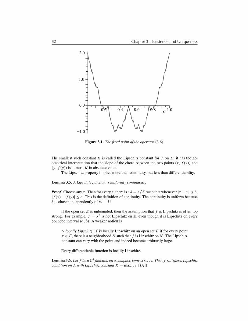
Example:As a slightly more interesting example, consider the same function space but let
T (f )(x) = cos(2πx) + 12f (2x). (3.6)
Note that T decreases the sup-norm by a factor of 1/2 as before, so it is still contracting. Forexample, the sequence starting with the function fo(x) = sin(2πx) is
f1(x) = cos(2πx) + 12
sin(4πx),
f2(x) = cos(2πx) + 12
cos(4πx) + 14
sin(8πx),
fj (x) =j−1!
n=0
cos(2n+1πx)
2n+ 1
2jsin(2j+1πx).
The last term goes to zero in the sup-norm, and by the contraction-mapping theorem, theresult is guaranteed to be unique and continuous. The fixed point is not an elementaryfunction but is easy to graph; see Figure 3.1; it is an example of a Weierstrass function(Falconer 1990).
Lipschitz Functions
Another ingredient that we will need in the existence and uniqueness theorem is a notionthat is stronger than continuity but slightly less stringent than differentiability:
◃ Lipschitz: Let E be an open subset of Rn. A function f : E → Rn isLipschitz if for all x, y ∈ E, there is a K such that
|f (x)− f (y)| ≤ K |x − y| . (3.7)
82 Chapter 3. Existence and Uniqueness
x 1.00.80.60.40.2
−1.0
1.0
2.0
0.0
Figure 3.1. The fixed point of the operator (3.6).
The smallest such constant K is called the Lipschitz constant for f on E; it has the ge-ometrical interpretation that the slope of the chord between the two points (x, f (x)) and(y, f (y)) is at most K in absolute value.
The Lipschitz property implies more than continuity, but less than differentiability.
Lemma 3.5. A Lipschitz function is uniformly continuous.
Proof. Choose any x. Then for every ε, there is a δ = ε!
K such that whenever |x − y| ≤ δ,|f (x)− f (y)| ≤ ε. This is the definition of continuity. The continuity is uniform becauseδ is chosen independently of x.
If the open set E is unbounded, then the assumption that f is Lipschitz is often toostrong. For example, f = x2 is not Lipschitz on R, even though it is Lipschitz on everybounded interval (a, b). A weaker notion is
◃ locally Lipschitz: f is locally Lipschitz on an open set E if for every pointx ∈ E, there is a neighborhood N such that f is Lipschitz on N . The Lipschitzconstant can vary with the point and indeed become arbitrarily large.
Every differentiable function is locally Lipschitz.
Lemma 3.6. Let f be aC1 function on a compact, convex setA. Then f satisfies a Lipschitzcondition on A with Lipschitz constant K = maxx∈A ∥Df ∥.
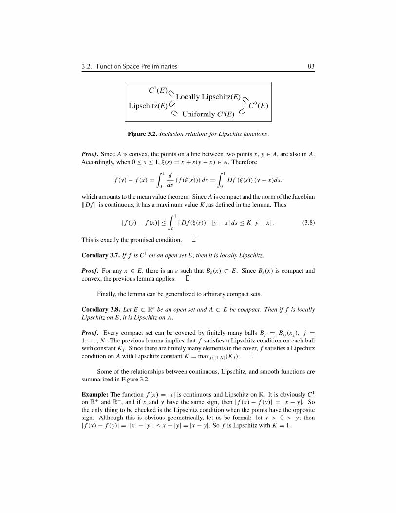
3.2. Function Space Preliminaries 83
C1(E)Locally Lipschitz(E)
Lipschitz(E) C 0 (E)Uniformly C0(E)
⊂⊂
⊂⊂ ⊂
Figure 3.2. Inclusion relations for Lipschitz functions.
Proof. Since A is convex, the points on a line between two points x, y ∈ A, are also in A.Accordingly, when 0 ≤ s ≤ 1, ξ(s) = x + s(y − x) ∈ A. Therefore
f (y)− f (x) =! 1
0
d
ds(f (ξ(s))) ds =
! 1
0Df (ξ(s)) (y − x)ds,
which amounts to the mean value theorem. Since A is compact and the norm of the Jacobian∥Df ∥ is continuous, it has a maximum value K , as defined in the lemma. Thus
|f (y)− f (x)| ≤! 1
0∥Df (ξ(s))∥ |y − x| ds ≤ K |y − x| . (3.8)
This is exactly the promised condition.
Corollary 3.7. If f is C1 on an open set E, then it is locally Lipschitz.
Proof. For any x ∈ E, there is an ε such that Bε(x) ⊂ E. Since Bε(x) is compact andconvex, the previous lemma applies.
Finally, the lemma can be generalized to arbitrary compact sets.
Corollary 3.8. Let E ⊂ Rn be an open set and A ⊂ E be compact. Then if f is locallyLipschitz on E, it is Lipschitz on A.
Proof. Every compact set can be covered by finitely many balls Bj = Bsj(xj ), j =
1, . . . , N . The previous lemma implies that f satisfies a Lipschitz condition on each ballwith constant Kj . Since there are finitely many elements in the cover, f satisfies a Lipschitzcondition on A with Lipschitz constant K = maxj∈[1,N ](Kj ).
Some of the relationships between continuous, Lipschitz, and smooth functions aresummarized in Figure 3.2.
Example: The function f (x) = |x| is continuous and Lipschitz on R. It is obviously C1
on R+ and R−, and if x and y have the same sign, then |f (x)− f (y)| = |x − y|. Sothe only thing to be checked is the Lipschitz condition when the points have the oppositesign. Although this is obvious geometrically, let us be formal: let x > 0 > y; then|f (x)− f (y)| = ||x|− |y|| ≤ x + |y| = |x − y|. So f is Lipschitz with K = 1.
84 Chapter 3. Existence and Uniqueness
However, the function f (x) = |x|1/2 is not Lipschitz on any interval containing 0.For example, choosing x = 4ε, y = −ε, we then have
|f (x)− f (y)| =!
|x|−!
|y| = √ε = ε√ε
= 1√ε
4ε − (−ε)5
= 15√ε
|x − y| ,
so that as ε becomes small, the needed value of K →∞.
All these formal definitions have been given to provide us with the tools to prove thatsolutions to certain ODEs exist and, if the initial values are given, are unique. We are finallyready to begin this analysis.
3.3 Existence and Uniqueness TheoremBefore we can begin to study properties of the solutions of differential equations, we mustdiscover if there are solutions in the first place: do solutions exist? The foundation of thetheory of differential equations is the theorem proved by the French analyst Charles EmilePicard in 1890 and the Finnish topologist Ernst Leonard Lindelöf in 1894 that guaranteesthe existence of solutions for the initial value problem
x = f (x), x(to) = xo (3.9)
for a solution x : R → Rn and vector field f : Rn → Rn. We were able to avoid thisdiscussion in Chapter 2 because linear differential equations can be solved explicitly. Sincethis is not the case for more general ODEs, we must now be more careful.
The main tool that we will use in developing the theory is the reformation of thedifferential equation as an integral equation. Formally integrating the ODE in (3.9) withrespect to t yields
x(t) = xo +" t
t0
f (x(τ ))dτ . (3.10)
This equation, while correct, is actually not a “solution” for x(t) since in order to find x,the integral on the right-hand side must be computed—but this requires knowing x.
Begin by imagining that (3.10) can be solved to find a function
x : J → Rn
on some time interval J = [to − a, to + a]. Since the integral in (3.10) does not requiredifferentiability of x(τ ), we will only assume that it is continuous. However, given thatsuch a solution x(t) to (3.10) exists, then it is actually a solution to the ODE (3.9).
Lemma 3.9. Suppose f ∈ Ck(E, Rn) for k ≥ 0 and x ∈ C0(J, E) is a solution of (3.10).Then x ∈ Ck+1(J, E) and is a solution to (3.9).
Proof. First note that if x solves (3.10), then x(to) = xo. Since x ∈ C0(J ), the integrandf (x(τ )) is also continuous and so the right-hand side of (3.10), being the integral of acontinuous function, is C1; consequently, the left-hand side of (3.10), x(t), is also differ-entiable. By the fundamental theorem of calculus, the derivative of the right-hand side is