27

Chapter 3Evolutionary Algorithms Based on Structured Coding

for Aerodynamic Wing Optimizations

3.1 IntroductionThe difficulty in finding the global optimum in an aerodynamic shape design optimization

problem stems in a large part from its high degree of nonlinearity in the objective functiondistribution. When EAs are used to solve engineering optimization problems, the term epistasis isoften used to describe nonlinearity in the objective function distribution [1]. In highly epistaticproblems, many of the design parameters strongly interact with each other and thus, it is very difficultto decompose such design problem into independent subproblems. Since EAs typically optimize bycombining valid features (sets of dependent parameters) of different design candidates, the robustnessand efficiency of EAs decrease significantly for such design problems. Therefore, if the epistaticinteraction structures of the design parameters are identified in advance, the robustness and efficiencyof EAs can work more robustly and efficiently by rearranging encoding of the design parameters.

To illustrate this, consider two sequentially coded design candidates (Parent1&2) where thereare strong interactions between real design variables a and e as well as b and d (Fig. 3.1).

a1 a2

b 1

c2c1

b 2

d 1 d 2

e1 e2

Sequential coding

Parent 1 Parent 2

Fig. 3.1 Sequentially coded design candidatesApplication of one-point crossover at any site would wind up destroying the above combinations. Insuch a case EAs would not work well. Consider now an alternative arrangement, in which interactivedesign parameters are grouped as Fig. 3.2.

28

Structured coding

P 1 P2

Q 1 Q 2

Parent 1 Parent 2

c 2c 1

a 1

b 1

c 1

d 1

e 1

a 2

b 2

c 2

d 2

e 2

Fig. 3.2 Design candidates coded with structure

In this case, no matter whether one-point crossover is applied to between P and Q or between Q and c,the combinations of the dependent design parameters are preserved.

For analysis of concerning design problems, a parametric study is often conducted by varyingone parameter at a time or by trial and error for a limited number of parameters. However, suchapproaches only lead to incomplete knowledge for a large design space. An exhaustive search, incontrast, requires unacceptably large number of experiments and thus they are not suitable to real-world problems. For instance, a full factorial design of a design space of 10 parameters with 3 levelswould require 310 = 59049 experiments. The use of such a time consuming approach is prohibitive forthe preprocessing epistasis analysis.

An efficient approach is experimental design that can gain required information at the leastexpenditure of resources. The underlying idea of this statistical technique is that the number ofexperiments can be reduced by extracting the required information, often the main effects and 2-factorinteractions, assuming that higher order of interactions are negligible in typical design problems. Thistechnique construct algebraic approximations of the objective function distribution with a set ofexperiments carefully distributed throughout the design space using so-called orthogonal array andthen, the effectiveness of the factors and their interactions are estimated by F-tests (for more detail, see[2])

The objective of this chapter is to improve robustness as well as efficiency of EAs byintroducing the structured coding based on the epistasis analysis. Experimental design will be used toexamine the epistatic interaction structures of design parameters. First, feasibility of typical airfoilshape parameterization techniques will be examined though reproduction of a NASA supercriticalairfoil and an aerodynamic airfoil shape optimization in Sec. 3.2. Then, the present approach will beapplied to aerodynamic design of a wing shape in Sec 3.3.

3.2 Comparative Study of Airfoil Shape Parameterization TechniquesIn recent years, the development of automated design process for aerodynamic design is

actively studied by many researchers. For instance, more than twenty papers related to aerodynamic ormultidisciplinary optimization by numerical methods were presented in the 38th AIAA aerospacesciences meeting and exhibit held on January 2000. In spite of such vigorous investigations, as is thecase in any new research field, many questions remain unanswered. Parameterization of the designspace, as well as choice of optimization methods, is one of the most outstanding issues of concern.

There are three objectives in developing a parameterization technique:1) A parameterization technique should have adequate flexibility. Otherwise, the global optimum

design may be excluded from the design space. For example, if a transonic airfoil shape weredesigned using NACA four-digit airfoils, the obtained airfoil would have high wave drag under a

29

certain thickness constraint.2) The number of required parameters should be kept as low as possible since it corresponds to the

number of dimensions of a design space. An extreme example is reported in [3] where a three-dimensional wing shape was parameterized by using the location of each surface mesh point asdesign parameters. This approach required more than 4000 design parameters. The final result wastherefore subject to constraints and the additional geometry smoothing. It is not efficient to find aglobal optimum design in such a large design space.

3) Design parameters should control important features of the given design problem. Because suchparameters are likely to be independent of each other, optimization can be conducted efficiently.One may recall that early studies on airfoil properties in subsonic flow were efficientlydemonstrated by dividing an airfoil shape into thickness distribution and camber line. On the otherhand, a design parameter set that is chosen without knowledge of the given design problem wouldhave complex interaction among them providing a complex objective function landscape. Findinga global optimum is very difficult in such an optimization problem.

Although many researchers have proposed airfoil shape parameterization techniques to achieve theirgoals, there is no comparative study of airfoil shape parameterization techniques aside from a work ofReuther and Jameson [4] within the author’s knowledge. In this section, some typical airfoilparameterization techniques will be compared to clarify this open issue.

3.2.1 Airfoil Shape Parameterization Techniques3.2.1.1 Extended Joukowski Transformation

Equation (3.1) is well known as the Joukowski transformation that transforms a circle intovarious airfoils:

zz

1+=ς (3.1)

The extended Joukowski transformation [5] gives further variety in the resultant airfoil shapes using apreliminary transformation before the Joukowski transformation as:

)( ∆−−=′

zzz ε

(3.2)

zz ′+′= 1ς (3.3)

where ε and ∆ are a complex number and a real number, respectively. The airfoil shape is defined by 5parameters: center of the circle Zc, real part and imaginary part of ε, and ∆. An example of theextended Joukowski transformation is illustrated in Fig. 3.3.

Instead of the raw design variables (Zc, ε, ∆), the present design variables are given by (xc, yc,xt, yt, ∆) where the center of the circle Zc and the complex number ε correspond to the position (xc, yc)and (xt, yt), respectively. ∆ is the preliminary movement in the real axis. It is known that xc and xt arerelated to the airfoil thickness while yc and yt are related to the airfoil camber.

3.2.1.2 Inverse Theodorsen TransformationAny given airfoil shape can be transformed into a unit circle using the Theodorsen

transformation [6] that consists of the following Joukowski transformation and the primaryapproximation:

zz ′+′= 1ς (3.4)

30

)exp(0∑=′∞

nn

zc

zz (3.5)

where the complex numbers Cn are determined by the fast Fourier transformation. The inverse of theTheodorsen transformation can be used to parameterize an airfoil shape. The accuracy of thistechnique depends on the truncation of summation in Eq. (3.5). In this study, an airfoil shape isdefined by 13 parameters, which corresponds to the truncation at the sixth term.

-2

-1

0

1

2

-2 -1 0 1 2

ZZ'Zeta

Imag

RealFig. 3.3 Example of the extended Joukowski transformation

3.2.1.3 B-Spline CurvesParameterization using the third-order B-Spline curves is one of the most popular approaches

for airfoil designs (for example, see [7,8]). The design parameters are positions of control points of theB-Spline curves. In this study, an airfoil shape is split into a mean camber line and thicknessdistribution. Five control points are used for each of the mean camber line and the thicknessdistribution (Fig. 3.4). Since locations of the leading edge and trailing edge are frozen, 12 designvariables are required to give an airfoil shape.

31

Thickness distributionControl points for thickness distribution

0

0.02

0.04

0.06

0.08

0.1

Z/C

Camber lineControl points for camber line

0

0.02

0.04

0.06

0.08

0.1

Z/C

Airfoil shape

-0.05

0

0.05

0.1

0 0.2 0.4 0.6 0.8 1

Z/C

X/C

camber line thickness distribution

airfoil shape

Fig. 3.4 B-Spline curves for mean camber line and thickness distributionand the resultant airfoil shape

3.2.1.4 Orthogonal Shape FunctionsThere is a class of parameterization techniques based on linear combination of shape functions.

In Ref. 9, Chang et al. have proposed a polynomial function to parameterize upper and lower surfacesof an airfoil using orthogonal shape functions to reduce the required design parameters:

)()()( 5110

7

416

2

121

1−

=

−

=

− −+−+−= ∑∑ n

n

nn

n

nnn xxaxxaxxaZ (3.6)

This approach for the airfoil parameterization is a derivative of the original NACA method [10]. Thenumber of parameters is 20.

3.2.1.5 PARSEC AirfoilsAn airfoil family “PARSEC” has been recently proposed to parameterize an airfoil shape [11].

A remarkable point is that this technique has been developed aiming to control important aerodynamicfeatures effectively by selecting the design parameters based on the knowledge of transonic flowsaround an airfoil.

Similar to 4-digit NACA series airfoils, The PARSEC parameterizes upper and lower airfoilsurfaces using polynomials in coordinates X, Z as,

∑=

−⋅=6

1

2/1

n

nn XaZ (3.7)

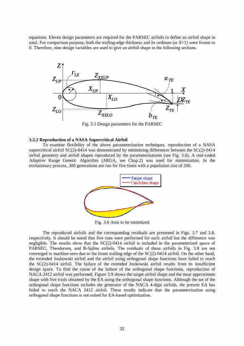
where an are real coefficients. Instead of taking these coefficients as design parameters, the PARSECairfoils are defined by basic geometric parameters: leading-edge radius, upper and lower crest locationincluding curvatures, trailing-edge ordinate, thickness, direction and wedge angle as shown in Fig. 3.5.These parameters can be expressed by the original coefficients an by solving simple simultaneous

32

equations. Eleven design parameters are required for the PARSEC airfoils to define an airfoil shape intotal. For comparison purpose, both the trailing-edge thickness and its ordinate (at X=1) were frozen to0. Therefore, nine design variables are used to give an airfoil shape in the following sections.

αTE

βTE

rLE

XUP

XLO

10

ZXXUP

ZXXLO

ZUP

ZLOZTE

∆ZTE

Z

X

αTE

βTE

rLE

XUP

XLO

10

ZXXUP

ZXXLO

ZUP

ZLOZTE

∆ZTE

Z

X

Fig. 3.5 Design parameters for the PARSEC

3.2.2 Reproduction of a NASA Supercritical AirfoilTo examine flexibility of the above parameterization techniques, reproduction of a NASA

supercritical airfoil SC(2)-0414 was demonstrated by minimizing differences between the SC(2)-0414airfoil geometry and airfoil shapes reproduced by the parameterizations (see Fig. 3.6). A real-codedAdaptive Range Genetic Algorithm (ARGA, see Chap.2) was used for minimization. In theevolutionary process, 300 generations are run for five times with a population size of 200.

Fig. 3.6 Area to be minimized

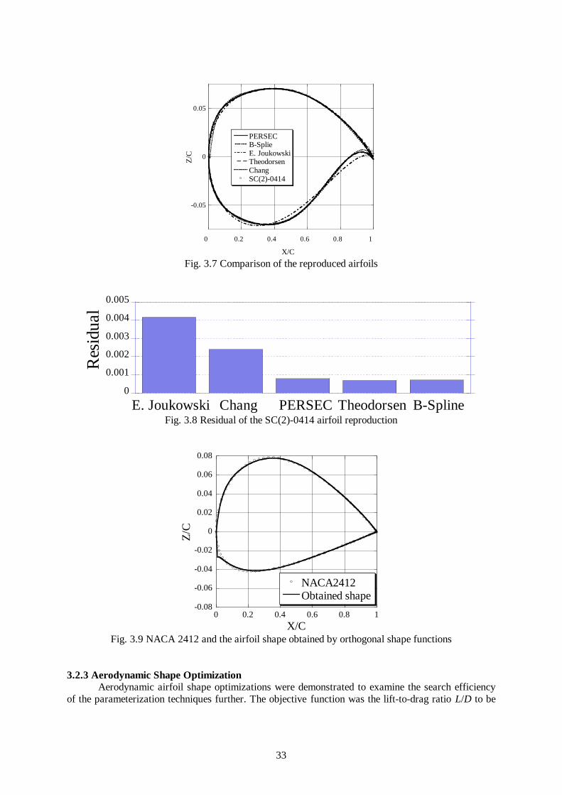
The reproduced airfoils and the corresponding residuals are presented in Figs. 3.7 and 3.8,respectively. It should be noted that five runs were performed for each airfoil but the difference wasnegligible. The results show that the SC(2)-0414 airfoil is included in the parameterized space ofPARSEC, Theodorsen, and B-Spline airfoils. The residuals of those airfoils in Fig. 3.8 are notconverged to machine-zero due to the brunt trailing edge of the SC(2)-0414 airfoil. On the other hand,the extended Joukowski airfoil and the airfoil using orthogonal shape functions have failed to reachthe SC(2)-0414 airfoil. The failure of the extended Joukowski airfoil results from its insufficientdesign space. To find the cause of the failure of the orthogonal shape functions, reproduction ofNACA 2412 airfoil was performed. Figure 3.9 shows the target airfoil shape and the most approximateshape with five trials obtained by the EA using the orthogonal shape functions. Although the set of theorthogonal shape functions includes the generator of the NACA 4-digit airfoils, the present EA hasfailed to reach the NACA 2412 airfoil. These results indicate that the parameterization usingorthogonal shape functions is not suited for EA-based optimization.

33

-0.05

0

0.05

0 0.2 0.4 0.6 0.8 1

PERSECB-SplieE. JoukowskiTheodorsenChangSC(2)-0414

Z/C

X/C

Fig. 3.7 Comparison of the reproduced airfoils

0

0.001

0.002

0.003

0.004

0.005

E. Joukowski Chang PERSEC Theodorsen B-Spline

Res

idua

l

Fig. 3.8 Residual of the SC(2)-0414 airfoil reproduction

-0.08

-0.06

-0.04

-0.02

0

0.02

0.04

0.06

0.08

0 0.2 0.4 0.6 0.8 1

NACA2412Obtained shape

Z/C

X/CFig. 3.9 NACA 2412 and the airfoil shape obtained by orthogonal shape functions

3.2.3 Aerodynamic Shape OptimizationAerodynamic airfoil shape optimizations were demonstrated to examine the search efficiency

of the parameterization techniques further. The objective function was the lift-to-drag ratio L/D to be

34

maximized. The free stream Mach number and the angle of attack were set to 0.8 and 2 degrees,respectively. The aerodynamic performance of each design was evaluated by the two-dimensionalNavier-Stokes solver described in Chap.4. The airfoil thickness was constrained so that the maximumthickness was greater than 12% of the chord length. The real-coded ARGA was used to maximize theobjective function where the population size and the number of generations were both 100. BecauseEAs are stochastic optimization algorithms, two trials were performed for each airfoilparameterization. Figure 3.10 shows the optimization histories. The aerodynamic performances of the designresults are summarized in Table 3.1. These results ensure that the performance of the designed airfoilgreatly depends on the choice of the parameterization techniques.

10

20

30

40

0 20 40 60 80 100

L/D

Generation

PERSECB-SplieE. JoukowskiTheodorsen

10

20

30

40

0 20 40 60 80 100

L/D

Generation

PERSECB-SplieE. JoukowskiTheodorsen

Fig. 3.10 Optimization histories

Table 3.1 Results of aerodynamic optimizationsTheodorsen Extended

JoukowskiB-Spline PARSEC

L/D 31.87 34.73 39.02 39.40Cl 0.5535 0.5427 0.6223 0.6253Cod 0.01737 0.01562 0.01595 0.01587

The present EA using the PARSEC airfoils has reached to the airfoil shape of the bestperformance. Because the parameter set of the PARSEC airfoils represents aerodynamically importantfeatures of an airfoil shape in transonic regime, they are to some extent independent and thus, thepresent EA could search the design space efficiently. This parameterization gives the design spacewide enough as shown in the previous section, which also helps finding a global optimum.

35

The resulting airfoil shape and the corresponding Cp distribution are shown in Fig. 3.11. Thesurface pressure distribution is similar to that of NASA supercritical airfoils, such as an approximatelyuniform distribution (rooftop) on the upper surface, a weak shock wave significantly aft of themidchord, a pressure plateau downstream of the shock wave, a relatively steep pressure recovery onthe extreme rearward region, and a trailing edge pressure slightly more positive than ambient pressure[12]. The design result is considered to be the global optimal and thus ensures the feasibility of thepresent approach.

-0.08

-0.06

-0.04

-0.02

0

0.02

0.04

0.06

0.08

-1.5

-1

-0.5

0

0.5

1

1.5

0 0.2 0.4 0.6 0.8 1

Z/C

-Cp

X/CFig. 3.11 Designed airfoil shape and the corresponding pressure distribution using PARSEC airfoils

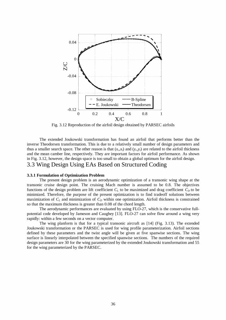
EA using the B-Spline curves has succeeded in finding a reasonably good airfoil design but theperformance of the resulting airfoil is slightly less than that optimized by the PARSEC airfoils. Thereason is probably the selection of the design parameters. The locations of B-Spline control points arenot related to the flow physics in contrast to the parameter set of the PARSEC airfoils. The resulting airfoil obtained from the inverse Theodorsen transformation performed worst. Tocheck whether the design obtained by the PARSEC airfoils is included in the search space of theinverse Theodorsen transformation, airfoil reproduction was tried as shown in Fig. 3.12. While theextended Joukowski airfoil has failed to express the best design, the others including the inverseTheodorsen transformation have succeeded. This indicates that the worst performance of EA using theinverse Theodorsen transformation is not due to its insufficient search space but the complex objectivefunction distribution. Because the parameters of the inverse Theodorsen transformation are not definedbased on the flow physics around an airfoil, they are likely to have complex interaction of each other.Because EAs typically optimize by combining valid features (sets of dependent parameters) ofdifferent design candidates, the robustness and efficiency of EAs decrease significantly for suchdesign problems.

36

-0.12

-0.08

-0.04

0

0.04

0 0.2 0.4 0.6 0.8 1

SobieczkyE. Joukowski

B-SplineTheodorsen

Z/C

X/CFig. 3.12 Reproduction of the airfoil design obtained by PARSEC airfoils

The extended Joukowski transformation has found an airfoil that performs better than theinverse Theodorsen transformation. This is due to a relatively small number of design parameters andthus a smaller search space. The other reason is that (xc,xt) and (yc,yt) are related to the airfoil thicknessand the mean camber line, respectively. They are important factors for airfoil performance. As shownin Fig. 3.12, however, the design space is too small to obtain a global optimum for the airfoil design.3.3 Wing Design Using EAs Based on Structured Coding

3.3.1 Formulation of Optimization ProblemThe present design problem is an aerodynamic optimization of a transonic wing shape at the

transonic cruise design point. The cruising Mach number is assumed to be 0.8. The objectivesfunctions of the design problem are lift coefficient CL to be maximized and drag coefficient CD to beminimized. Therefore, the purpose of the present optimization is to find tradeoff solutions betweenmaximization of CL and minimization of CD within one optimization. Airfoil thickness is constrainedso that the maximum thickness is greater than 0.08 of the chord length.

The aerodynamic performances are evaluated by using FLO-27, which is the conservative full-potential code developed by Jameson and Caughey [13]. FLO-27 can solve flow around a wing veryrapidly: within a few seconds on a vector computer.

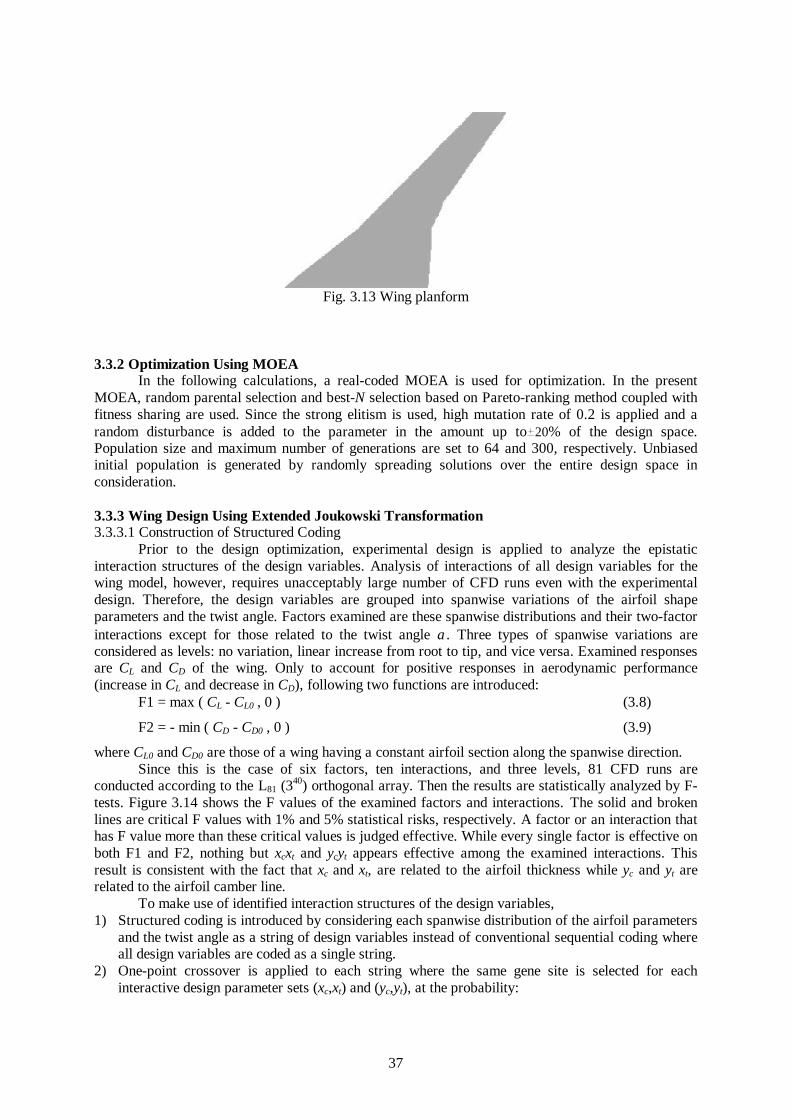
The wing planform is that for a typical transonic aircraft as [14] (Fig. 3.13). The extendedJoukowski transformation or the PARSEC is used for wing profile parameterization. Airfoil sectionsdefined by these parameters and the twist angle will be given at five spanwise sections. The wingsurface is linearly interpolated between the specified spanwise sections. The numbers of the requireddesign parameters are 30 for the wing parameterized by the extended Joukowski transformation and 55for the wing parameterized by the PARSEC.

37

Fig. 3.13 Wing planform

3.3.2 Optimization Using MOEAIn the following calculations, a real-coded MOEA is used for optimization. In the present

MOEA, random parental selection and best-N selection based on Pareto-ranking method coupled withfitness sharing are used. Since the strong elitism is used, high mutation rate of 0.2 is applied and arandom disturbance is added to the parameter in the amount up to 20% of the design space.Population size and maximum number of generations are set to 64 and 300, respectively. Unbiasedinitial population is generated by randomly spreading solutions over the entire design space inconsideration.

3.3.3 Wing Design Using Extended Joukowski Transformation3.3.3.1 Construction of Structured Coding

Prior to the design optimization, experimental design is applied to analyze the epistaticinteraction structures of the design variables. Analysis of interactions of all design variables for thewing model, however, requires unacceptably large number of CFD runs even with the experimentaldesign. Therefore, the design variables are grouped into spanwise variations of the airfoil shapeparameters and the twist angle. Factors examined are these spanwise distributions and their two-factorinteractions except for those related to the twist angle α. Three types of spanwise variations areconsidered as levels: no variation, linear increase from root to tip, and vice versa. Examined responsesare CL and CD of the wing. Only to account for positive responses in aerodynamic performance(increase in CL and decrease in CD), following two functions are introduced:

F1 = max ( CL - CL0 , 0 ) (3.8)

F2 = - min ( CD - CD0 , 0 ) (3.9)

where CL0 and CD0 are those of a wing having a constant airfoil section along the spanwise direction.Since this is the case of six factors, ten interactions, and three levels, 81 CFD runs are

conducted according to the L81 (340) orthogonal array. Then the results are statistically analyzed by F-tests. Figure 3.14 shows the F values of the examined factors and interactions. The solid and brokenlines are critical F values with 1% and 5% statistical risks, respectively. A factor or an interaction thathas F value more than these critical values is judged effective. While every single factor is effective onboth F1 and F2, nothing but xcxt and ycyt appears effective among the examined interactions. Thisresult is consistent with the fact that xc and xt, are related to the airfoil thickness while yc and yt arerelated to the airfoil camber line.

To make use of identified interaction structures of the design variables,1) Structured coding is introduced by considering each spanwise distribution of the airfoil parameters

and the twist angle as a string of design variables instead of conventional sequential coding whereall design variables are coded as a single string.

2) One-point crossover is applied to each string where the same gene site is selected for eachinteractive design parameter sets (xc,xt) and (yc,yt), at the probability:

38

))50/,1(min(7.01.0 generationprob += (3.10)

Figure 3.15 illustrates the proposed structured coding for the present wing shape modeling.The broken lines in the figure show how one-point crossover is applied to the present structuredcoding. This crossover enables that the genes of the identified parameter sets, such as (xc xt) and (yc yt)are exchanged together to utilize efficiently the effects of the interactions between them.

xc yc xt yt ∆ α xcyc xcxt xcyt xc∆ ycxt ycyt yc∆ xtyt xt∆ yt∆

Fig. 3.14 Effectiveness of factors and their interactions for the extended Joukowski transformation

X

Xc1

Xc2

Xc3

Xc5

Xc4

Y

Yc1

Yc2

Yc3

Yc5

Yc4

Xt1

Xt2

Xt3

Xt5

Xt4

∆

∆1

∆2

∆3

∆5

∆4

α

α1

α2

α3

α5

α4

Yt1

Yt2

Yt3

Yt5

Yt4

Profile1Profile2

Profile3

Profile4

Profile5

One-point Crossover gene siteFig. 3.15 Structured coding for the extended Joukowski transformation

3.3.3.2 Design Results

39

To validate advantage of the crossover with the structured coding, design optimization isdemonstrated. The design results obtained by the present approach are compared with that of the EAwith the sequential coding where one-point crossover is applied to each spanwise distribution of thedesign parameters but each crossover gene site is selected independently as illustrated in Fig. 3.16.Figure 3.17 shows the Pareto optimal solutions indicating the tradeoff between maximization of CL

and minimization of CD. Solid and hollow points show the resulting Pareto fronts obtained from thesequential and structured codings, respectively. This figure indicates that the present EA with thestructured coding had better Pareto solutions in high CL region.

Xc

Xc1

Xc2

Xc3

Xc5

Xc4

Yc

Yc1

Yc2

Yc3

Yc5

Yc4

Xt1

Xt2

Xt3

Xt5

Xt4

∆

∆1

∆2

∆3

∆5

∆4

α

α1

α2

α3

α5

α4

Yt1

Yt2

Yt3

Yt5

Yt4

Xt Yt

Profile1

Profile2

Profile3

Profile4

Profile5

One-point Crossover gene siteFig. 3.16 Sequential coding for the extended Joukowski transformation

0.2

0.3

0.4

0.5

0.6

0.7

0.8

0.9

1

0 0.01 0.02 0.03 0.04 0.05

sequentialstructured

CL

CD

Fig. 3.17 Comparison of Pareto fronts for sequential and structured coding techniques

3.3.4 Wing Design Using PARSEC Airfoils3.3.4.1 Construction of Structured Coding

Now, the present approach is applied to wing design using the PARSEC. First, the interactionstructures of the parameter sets for the PARSEC airfoils are analyzed by the experimental design. Thefactors to be examined are rLE, XUP, ZUP, ZXXUP, XLO, ZLO, ZXXLO, αTE, ZTE and their two-factorinteractions on F1 and F2. The wedge angle at the trailing edge and its interactions are neglected sincethe wedge angle is primary determined by the structural strength. Also, interactions of rLEZTE, rLEαTE

and rLEZXXLO are disregarded. Consequently, 42 factors are examined by the experimental design

40

conducted according to the L729(3364) design template. Number of CFD runs required for this epistasisanalysis is reduced from 39 = 19683 (full factorial design) to 36 = 729.

Figure 3.18 shows the result of the F-tests. Interactions effective in both CL and CD areillustrated with bold lines in Fig. 3.19. Since these figures indicate complicated interactions among thedesign variables, especially, ZUP, ZLO, and ZTE, it seems difficult to construct a structured coding forthese design variables. Therefore, new parameters ZC and ZH are introduced instead of ZUP and ZLO as:

ZC = ( ZUP + ZLO ) / 2 (3.11)

ZH = ( ZUP - ZLO ) (3.12)

where ZC and ZH correspond to airfoil camber and thickness, respectively. Using these parameters,interactions are greatly simplified as shown in Fig. 3.20. According to this result, a structured codingfor the spanwise distributions of airfoil parameters is introduced.

0

1

2

3

4

5

6

7

8

9

10

1 3 5 7 9 11 13 15 17 19 21 23 25 27 29 31 33Factors and interactions

F

CL CD Critical Value(1%) Critical Value(5%)

XLO XLO XLO ZLO ZLO ZLO ZLO ZTE ZTE ZTE αTE ZUP ZLO ZTE ZUP ZTE αTE ZUP XUP αTE ZUP XUP ZUP XUP

Fig. 3.18 Effectiveness of factors and their interactions for the PARSEC

rLE

XLO

XUPZXXUP

ZXXLO

αTE

ZTE

ZUP

ZLOFig. 3.19 Effective interactions of the original PARSEC

41

rLE

XLO

XUPZXXUP

ZXXLO

αTE

ZTE

ZTH

ZCFig. 3.20 Effective interactions of the modified PARSEC

3.3.4.2 Design ResultsThe design result obtained by the EA using the crossover based on the structured coding is

compared with that obtained by the EA using the sequential coding. Figure 3.21 compares Paretofronts obtained from the sequential coding of the original PARSEC airfoils and the structured codingusing ZC and ZH. Similar to the previous section using the extended Joukowski airfoils, advantage ofthe crossover based on the structured coding is observed in high CL region. Compared with Fig. 3.17,this figure also illustrated that Pareto front of the PARSEC airfoils is superior to that of the extendedJoukowski airfoils.

0.2

0.3

0.4

0.5

0.6

0.7

0.8

0.9

1

0 0.01 0.02 0.03 0.04 0.05

sequentialstructured

CL

CD

Fig. 3.21 Comparison of Pareto fronts for sequential and structured coding techniques3.4 Summary

First, feasibility of typical airfoil shape parameterization techniques was investigated throughcomparative studies. The reproduction of a NASA supercritical airfoil showed that the extendedJoukowski airfoil was not insufficient for transonic airfoil shape designs. This study also showed thatthe parameterization using orthogonal shape functions is not suited for EA-based optimizations.

The aerodynamic airfoil shape optimizations ensured that the performance of the designedairfoil greatly depends on the choice of the parameterization techniques. EA using the PARSECairfoils succeeded in finding the airfoil shape of the best performance, thanks to the selection of design

42

parameters based on the knowledge of transonic flow around an airfoil. Because the parameter set ofthe PARSEC airfoils represents important features of the given design problem, they likely to beindependent of each other and thus, the present EA searched the design space efficiently.

On the other hand, design parameters of the inverse Theodorsen transformation that are chosenwithout knowledge of the flow physics around an airfoil provided a complex objective functionlandscape. Because EAs typically optimize by combining valid features of different design candidates,the performance of EAs decreases significantly for such design problems.

Then, a crossover operator based on structured coding has been proposed for EAs. The codingstructure of the design variables is developed according to the epistasis analyzed by the experimentaldesign. The present approach was applied to an aerodynamic shape design of a transonic wing wherethe wing shape is modeled using the parameter sets defined by the extended Joukowski airfoils and bythe PARSEC airfoils. Aerodynamic optimizations of a transonic wing demonstrated that the structuredcoding for EAs is a promising approach to find a global optimum in practical applications. The designresults also confirm that the PARSEC is an adequate technique for transonic wing shapeparameterization. The improved Pareto front is obtained by EA based on the proposed structuredcoding using the PARSEC.

43

References[1] Davidor, Y., Genetic Algorithms and Robotics: A Heuristic Strategy for Optimization, WorldScientific, Singapore, 1991, Chap. 9.[2] Barker, T. B., Quality by Experimental Design, Second edition, Marcel Dekker, Inc., New York,1994.[3] Jameson, A., “Optimum Aerodynamic Design via Boundary Control,” AGARD-VKI LectureSeries, Optimum Design Methods in Aerodynamics, von Karman Inst. For Fluid Dynamics, Rhode SaitGenese, Belgium, 1994.[4] Reuther, J. J. and Jameson, A., “A Comparison of Design Variables for Control Theory BasedAirfoil Optimization,” sixth International Symposium on Computational Fluid Dynamics, Lake Tahoe,Nevada, Sept. 1995.[5] Jones, R. T., Wing Theory, Princeton University Press, Princeton, NJ, 1990, Chap. 3.[6] Theodorsen, T. and Garrick, I. E. “General Potential Theory of Arbitrary Wing Sections,” NACATR 452, 1933.[7] Obayashi, S., “Pareto Genetic Algorithm for Aerodynamic Design Using the Navier-StokesEquations,” Genetic Algorithms and Evolution Strategy in Engineering and Computer Science, JohnWiley & Sons, Ltd, Chichester, U.K., 1998, pp.245-266.[8] Doorly, D. J. and Peiro, J., “Supervised Parallel Genetic Algorithms in AerodynamicOptimization,” AIAA-97-1852, 1997.[9] Chang, I., Torres, F. J. and Tung C., “Geometric Analysis of Wing Sections,” NASA TM 110346,1995.[10] Abbott, I. and von Doenhoff, A., Theory of Wing Sections, Dover Publications, New York, 1949.[11] Sobieczky, H, “Parametric Airfoils and Wings,” Recent Development of Aerodynamic DesignMethodologies –Inverse Design and Optimization –, Friedr. Vieweg & Sohn Verlagsgesellschaft mbH,Braunschweig/Wiesbaden, Germany, 1999, pp.72-74.[12] Harris, C. D., “NASA Supercritical Airfoils,” NASA TP 2969, 1990.[13] Jameson, A. and Caughey, D. A., “A Finite Volume Method for Transonic Potential FlowCalculations,” AIAA Paper 77-677, 1977.[14] Jacobs, P. F., “Experimental Trim Drag Values and Flow-Field Measurements or a Wide-BodyTransport Model with Conventional and Supercritical Wings,” NASA TP 2071, 1982.