Chapter 3 Discrete Time and State Models. Discount Functions

Chapter 3 Discrete Time and State Models

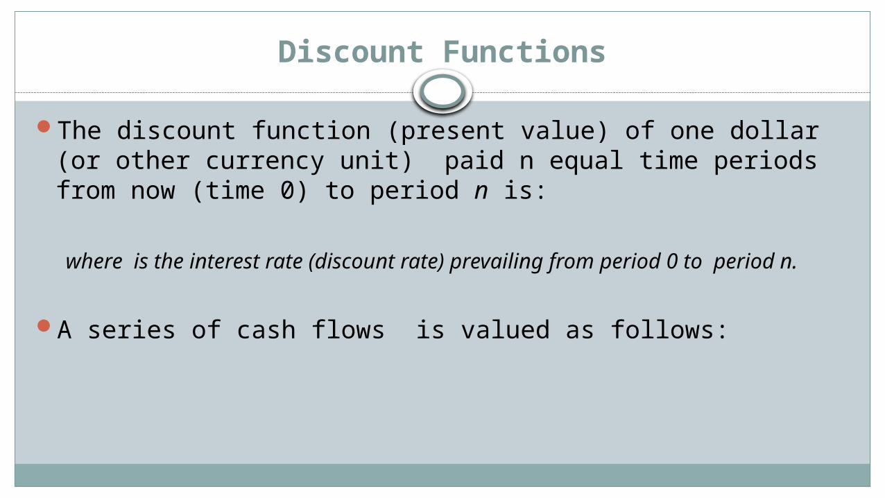
Discount Functions

The discount function (present value) of one dollar (or other currency unit) paid n equal time periods from now (time 0) to period n is:

where is the interest rate (discount rate) prevailing from period 0 to period n.

A series of cash flows is valued as follows:

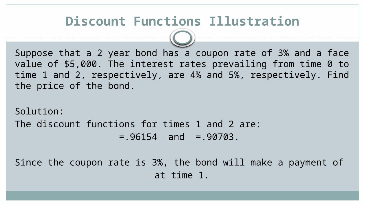
Discount Functions Illustration

Suppose that a 2 year bond has a coupon rate of 3% and a face value of $5,000. The interest rates prevailing from time 0 to time 1 and 2, respectively, are 4% and 5%, respectively. Find the price of the bond.

Solution: The discount functions for times 1 and 2 are:

=.96154 and =.90703.

Since the coupon rate is 3%, the bond will make a payment of at time 1.

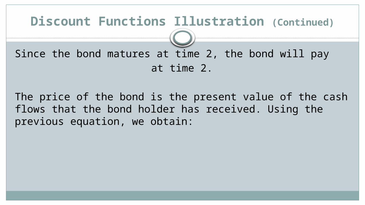
Discount Functions Illustration (Continued)

Since the bond matures at time 2, the bond will pay at time 2.

The price of the bond is the present value of the cash flows that the bond holder has received. Using the previous equation, we obtain:

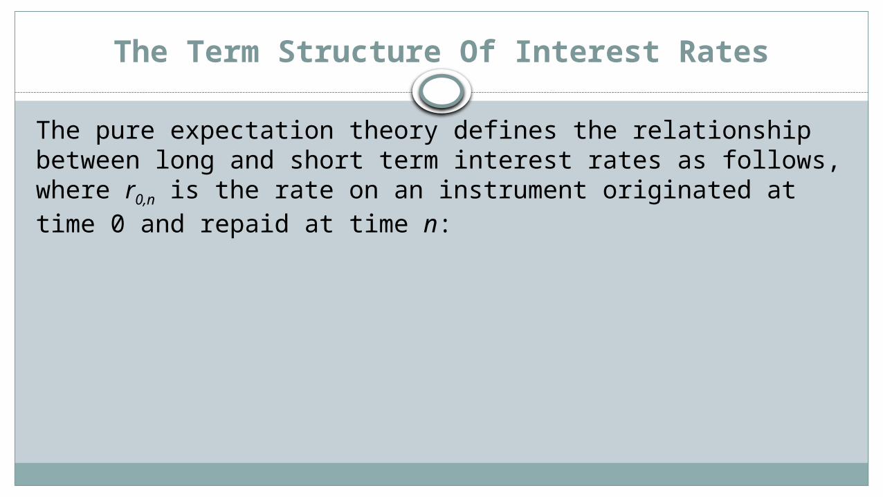
The Term Structure Of Interest Rates

The pure expectation theory defines the relationship between long and short term interest rates as follows, where r0,n is the rate on an instrument originated at time 0 and repaid at time n:

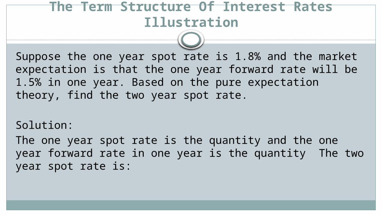
The Term Structure Of Interest Rates Illustration

Suppose the one year spot rate is 1.8% and the market expectation is that the one year forward rate will be 1.5% in one year. Based on the pure expectation theory, find the two year spot rate.

Solution: The one year spot rate is the quantity and the one year forward rate in one year is the quantity The two year spot rate is:

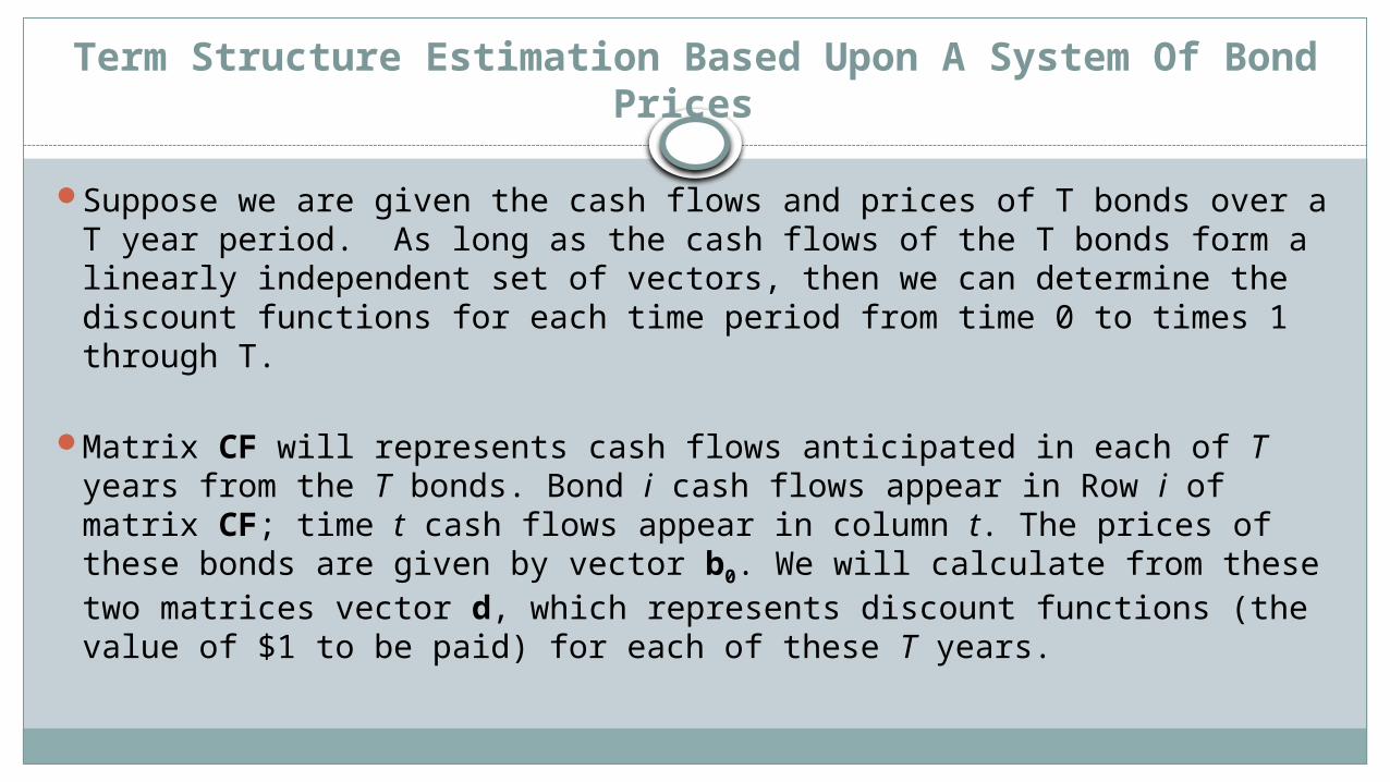
Term Structure Estimation Based Upon A System Of Bond Prices

Suppose we are given the cash flows and prices of T bonds over a T year period. As long as the cash flows of the T bonds form a linearly independent set of vectors, then we can determine the discount functions for each time period from time 0 to times 1 through T.

Matrix CF will represents cash flows anticipated in each of T years from the T bonds. Bond i cash flows appear in Row i of matrix CF; time t cash flows appear in column t. The prices of these bonds are given by vector b0. We will calculate from these two matrices vector d, which represents discount functions (the value of $1 to be paid) for each of these T years.

Term Structure Estimation Based Upon A System Of Bond Prices (continued)

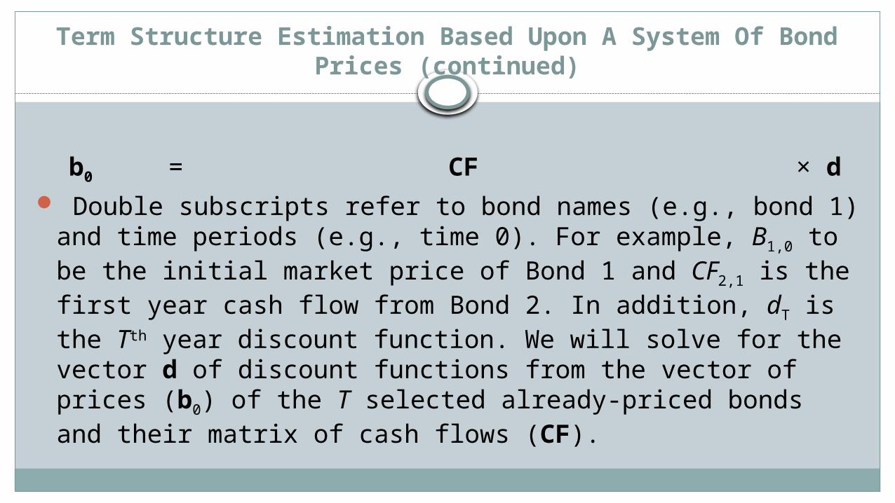
b0 = CF × d

Double subscripts refer to bond names (e.g., bond 1) and time periods (e.g., time 0). For example, B1,0 to be the initial market price of Bond 1 and CF2,1 is the first year cash flow from Bond 2. In addition, dT is the Tth year discount function. We will solve for the vector d of discount functions from the vector of prices (b0) of the T selected already-priced bonds and their matrix of cash flows (CF).


Once we have found d, we can then obtain interest rates, yield curves, and price any other bond that may enter the market in the T-year time frame. In order to obtain a unique solution for d, we need to have each row vector of the cash flow matrix be independent of one another. This is required because the inverse CF-1 of the matrix CF exists if and only if its row vectors are linearly independent. In that case, the solution for the vector of discount functions is given by:

d = CF-1 × b0


Any additional bonds entering the market can be priced based on the values of d. The financial interpretation of there existing T linearly independent cash flow vectors for T time periods is that the market satisfies the important requirement that bond markets be complete. If we were unable to find bonds that produced a set of T linearly independent cash flows, there would be insufficient information in the bond market in order to uniquely determine the discount functions, and hence the interest rates. Such markets are said to be incomplete.

Illustration

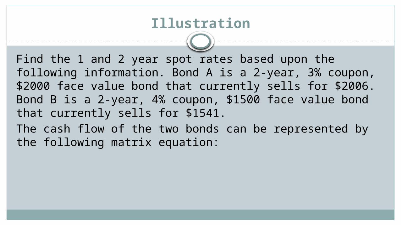
Find the 1 and 2 year spot rates based upon the following information. Bond A is a 2-year, 3% coupon, $2000 face value bond that currently sells for $2006. Bond B is a 2-year, 4% coupon, $1500 face value bond that currently sells for $1541.The cash flow of the two bonds can be represented by the following matrix equation:

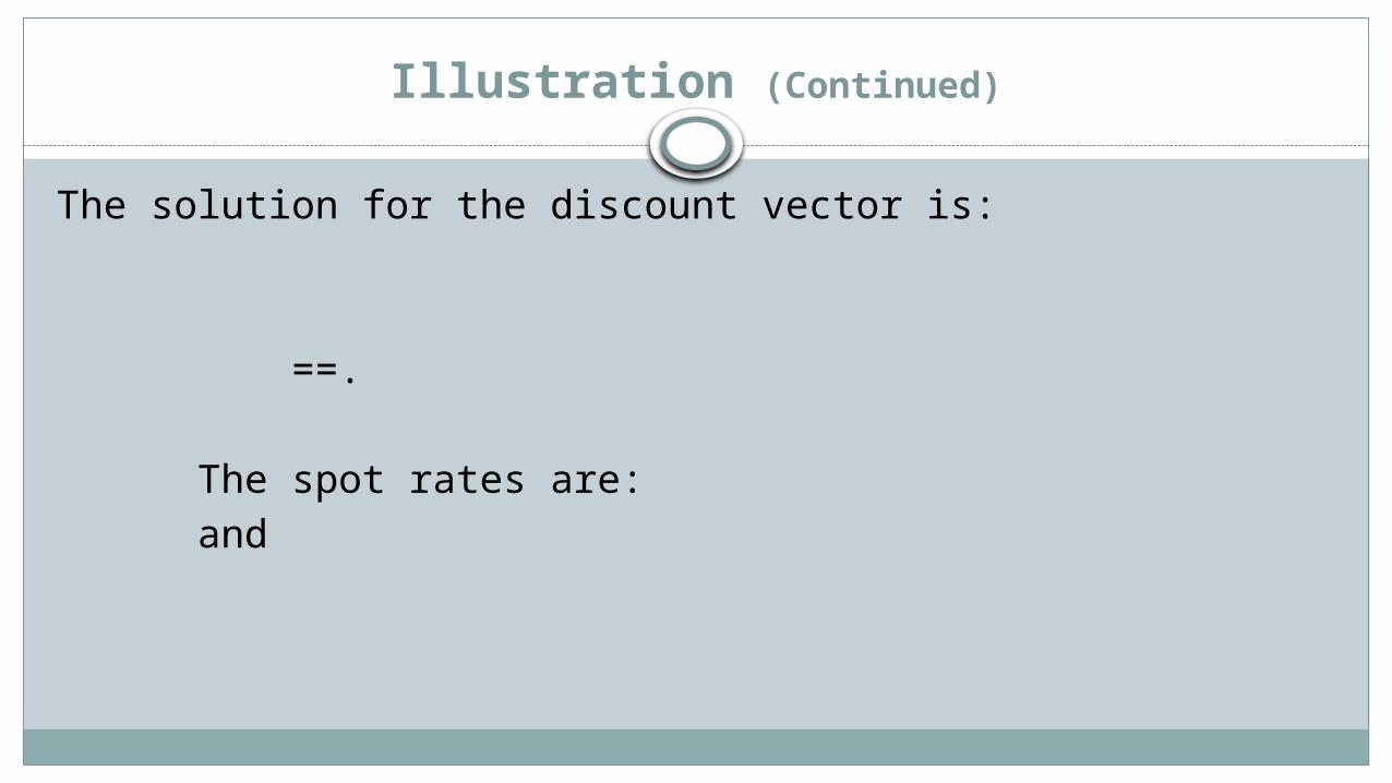
Illustration (Continued)

The solution for the discount vector is:

==.

The spot rates are: and

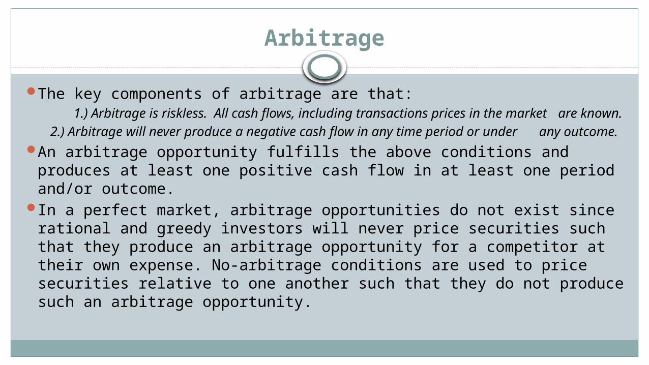
Arbitrage

The key components of arbitrage are that: 1.) Arbitrage is riskless. All cash flows, including transactions prices in the market are known. 2.) Arbitrage will never produce a negative cash flow in any time period or under any outcome. An arbitrage opportunity fulfills the above conditions and produces

at least one positive cash flow in at least one period and/or outcome. In a perfect market, arbitrage opportunities do not exist since

rational and greedy investors will never price securities such that they produce an arbitrage opportunity for a competitor at their own expense. No-arbitrage conditions are used to price securities relative to one another such that they do not produce such an arbitrage opportunity.

No-Arbitrage Bond Markets

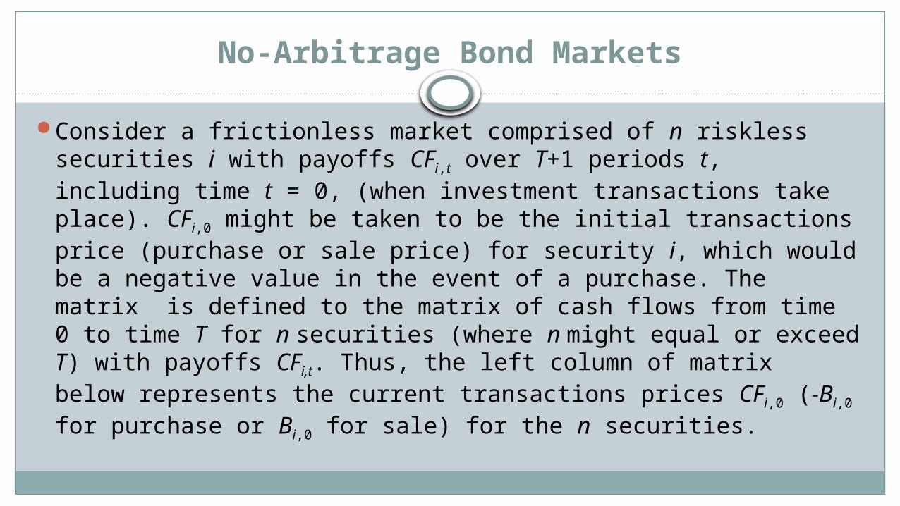
Consider a frictionless market comprised of n riskless securities i with payoffs CFi,t over T+1 periods t, including time t = 0, (when investment transactions take place). CFi,0 might be taken to be the initial transactions price (purchase or sale price) for security i, which would be a negative value in the event of a purchase. The matrix is defined to the matrix of cash flows from time 0 to time T for n securities (where n might equal or exceed T) with payoffs CFi,t. Thus, the left column of matrix below represents the current transactions prices CFi,0 (-Bi,0 for purchase or Bi,0 for sale) for the n securities.

No-Arbitrage Bond Markets (Continued)

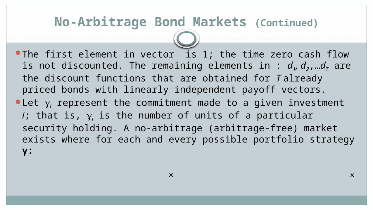
The first element in vector is 1; the time zero cash flow is not discounted. The remaining elements in : d1, d2,…dT are the discount functions that are obtained for T already priced bonds with linearly independent payoff vectors.

Let i represent the commitment made to a given investment i; that is, i is the number of units of a particular security holding. A no-arbitrage (arbitrage-free) market exists where for each and every possible portfolio strategy γ:

× ×

No-Arbitrage Bond Markets (Continued)

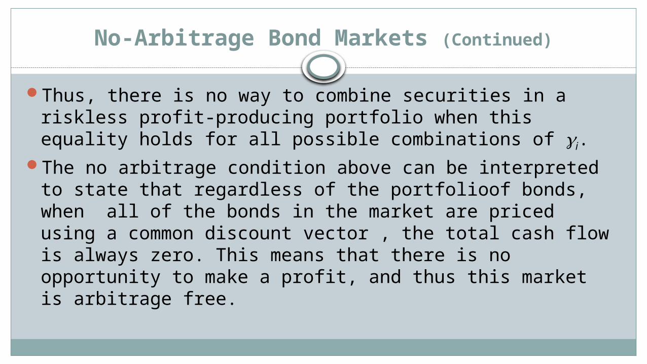
Thus, there is no way to combine securities in a riskless profit-producing portfolio when this equality holds for all possible combinations of i.

The no arbitrage condition above can be interpreted to state that regardless of the portfolioof bonds, when all of the bonds in the market are priced using a common discount vector , the total cash flow is always zero. This means that there is no opportunity to make a profit, and thus this market is arbitrage free.

Pricing Bonds In The Arbitrage-Free Market

In a market in which every bond is priced using the same set of discount functions, we observed that we must have an arbitrage free market.

Given an arbitrage free market over T time periods, if we have T already priced bonds with a linearly independent set of payoff vectors, we first determine the discount vector d. As we saw earlier, We can then price any bond in this market using this discount vector.

Continuing with the illustration earlier, find the price of a 2 year 1.5% coupon bond with face value of $1,000. The price of this bond must be:

$979.

Pricing Bonds In terms Already Priced Bonds

Typically, in a bond market, new bonds are priced based upon the prices of bonds that have already been priced in the market.

In a no arbitrage market with T time periods, as long as there are at least T bonds with linearly independent payoff vectors that have already been priced, then there is a consistent way to price any new bond entering the market.

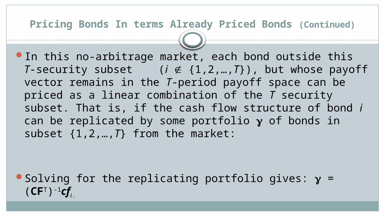
Pricing Bonds In terms Already Priced Bonds (Continued)

In this no-arbitrage market, each bond outside this T-security subset (i {1,2,…,T}), but whose payoff vector remains in the T-period payoff space can be priced as a linear combination of the T security subset. That is, if the cash flow structure of bond i can be replicated by some portfolio of bonds in subset {1,2,…,T} from the market:

Solving for the replicating portfolio gives: = (CFT)-1cfi.

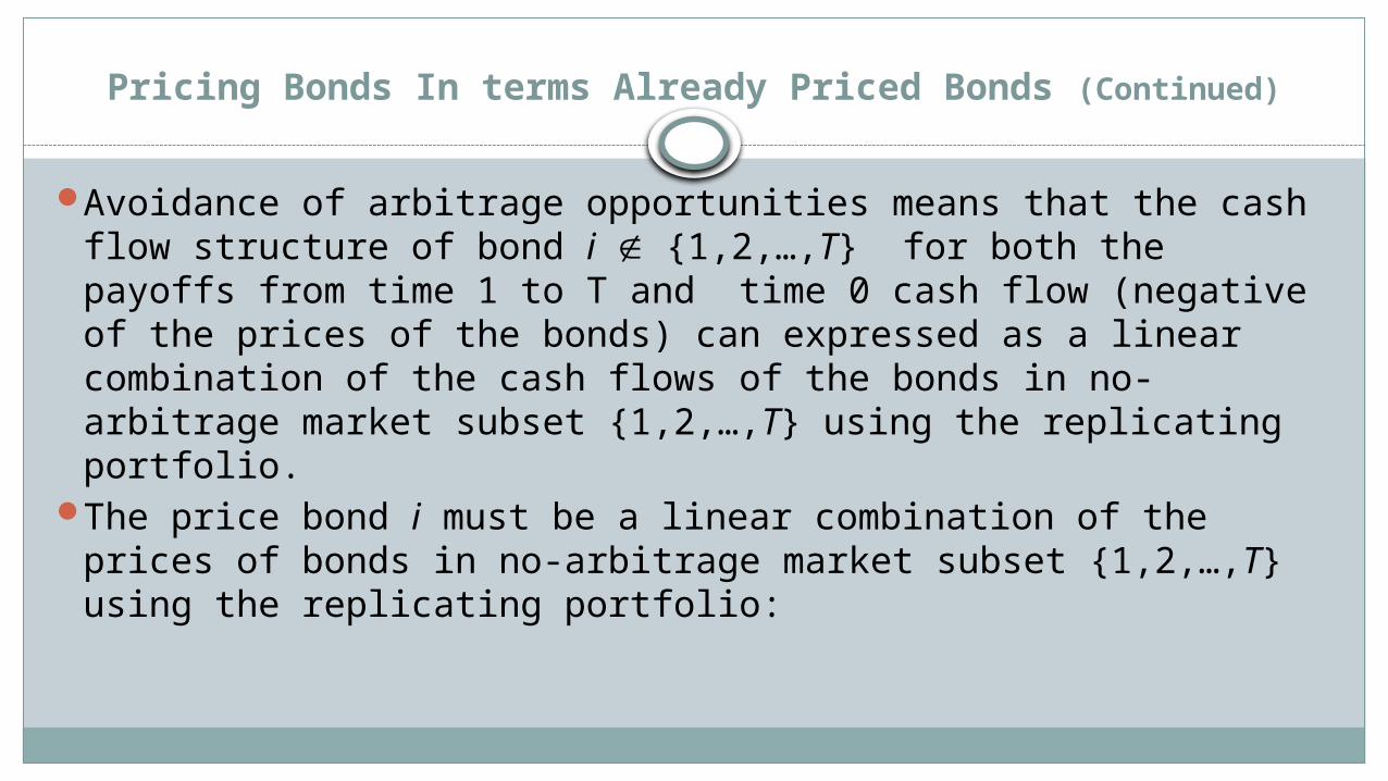
Pricing Bonds In terms Already Priced Bonds (Continued)

Avoidance of arbitrage opportunities means that the cash flow structure of bond i {1,2,…,T} for both the payoffs from time 1 to T and time 0 cash flow (negative of the prices of the bonds) can expressed as a linear combination of the cash flows of the bonds in no-arbitrage market subset {1,2,…,T} using the replicating portfolio.

The price bond i must be a linear combination of the prices of bonds in no-arbitrage market subset {1,2,…,T} using the replicating portfolio:

Illustration Of Pricing Bonds In terms Already Priced Bonds

We will price the bond from the previous illustration. We will see that we will obtain the same result as the discount method gave us. We wish to price a 2 year 1.5% coupon bond with a face value of $1000, which we will label as the third bond. It payoff vector is

We first solve for the replicating portfolio :

= (CFT)-1 x cf3

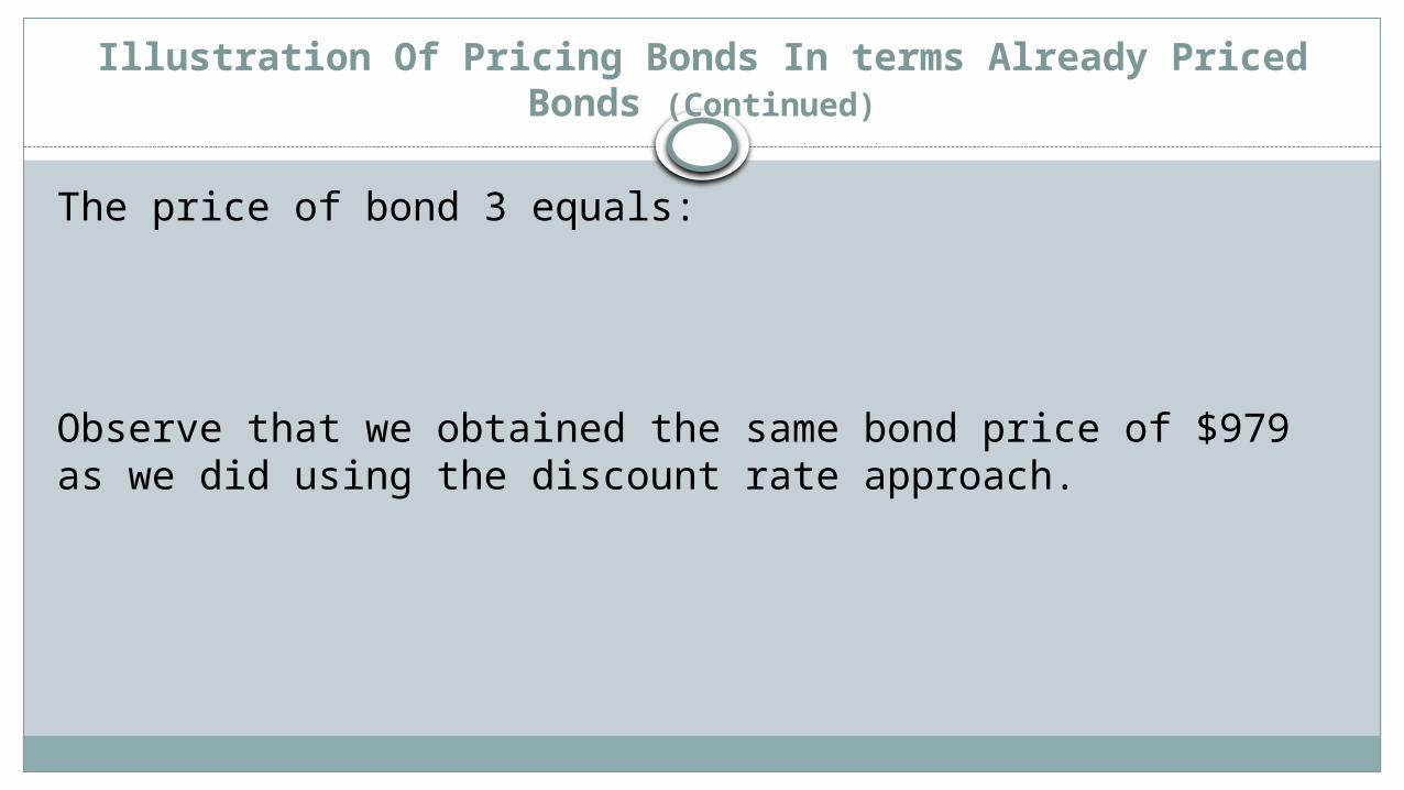
Illustration Of Pricing Bonds In terms Already Priced Bonds (Continued)

The price of bond 3 equals: Observe that we obtained the same bond price of $979 as we did using the discount rate approach.

Pure Securities

This process can involve determining the vector space ℝn, valuing n “control” securities with linearly independent payoff vectors, and pricing the payoff vectors of the previously unpriced securities based on linear combinations of prices from the “control” securities. We will initially assume the following for our valuations: 1.) There exist n potential states of nature (prices) in a one-time period framework. 2.) Each security will have exactly one payoff resulting from each potential state of nature.

Pure Securities (Continued)

3.) Only one state of nature will occur at the end of the period (states are mutually exclusive) and which state occurs is ex-ante unknown. 4.) Each investor's utility or satisfaction is a function only of his level of

wealth; the state of nature that is realized is important only to the extent that the investor's wealth is affected (this assumption can often be relaxed). 5.) Capital markets are in equilibrium (supply equals demand) for all securities.

Often, the states of nature are the possible outcomes in the future. For simplicity, we are assuming that there are only a finite number of possible future states. We will consider in later chapters the case when the number of possible future outcomes are unlimited (infinite).


Suppose that a given economy has n potential states of nature and there exists a security x with a known payoff vector:

Vector x defines every potential payoff for security x in this n-state

world. We will value this security based on known values of other securities existing in this three-state economy.

The first step in the evaluation procedure is to decompose the security into an imaginary portfolio of pure securities. Define a pure security (also known as an elementary, primitive or Arrow-Debreu security) to be an investment that pays $1 if and only if a particular outcome or state of nature is realized and nothing otherwise.


Thus, the payoff vector for a given pure security i in an n- potential outcome economy will comprise n elements such that:

1.) The ith element will equal 1. 2.) All other elements will equal zero. For example, the following is the payoff vector of pure

security 3 in an n- outcome economy:

Each security with a payoff vector in this n-dimensional payoff space can be replicated with the n pure securities from this space.

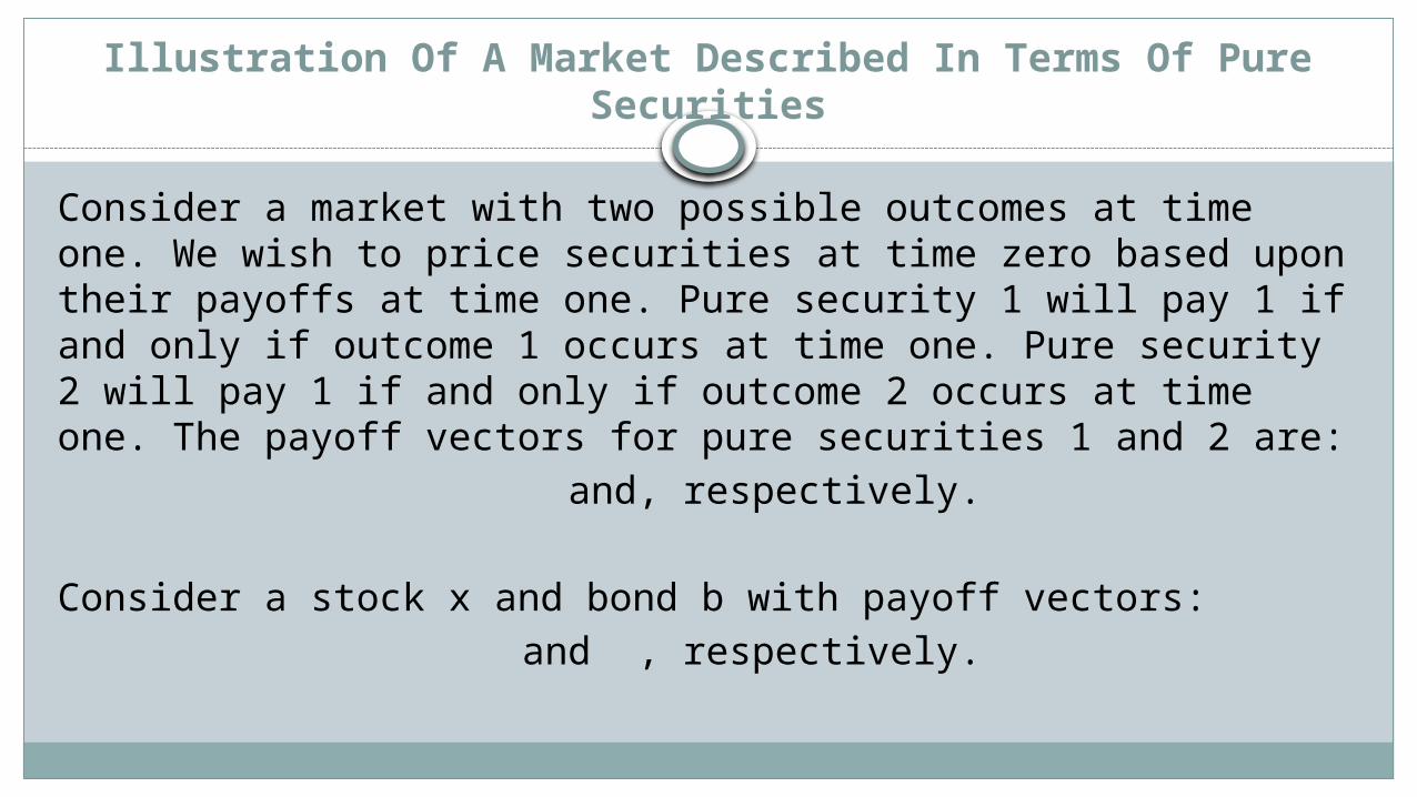
Illustration Of A Market Described In Terms Of Pure Securities

Consider a market with two possible outcomes at time one. We wish to price securities at time zero based upon their payoffs at time one. Pure security 1 will pay 1 if and only if outcome 1 occurs at time one. Pure security 2 will pay 1 if and only if outcome 2 occurs at time one. The payoff vectors for pure securities 1 and 2 are:

and, respectively.

Consider a stock x and bond b with payoff vectors: and , respectively.

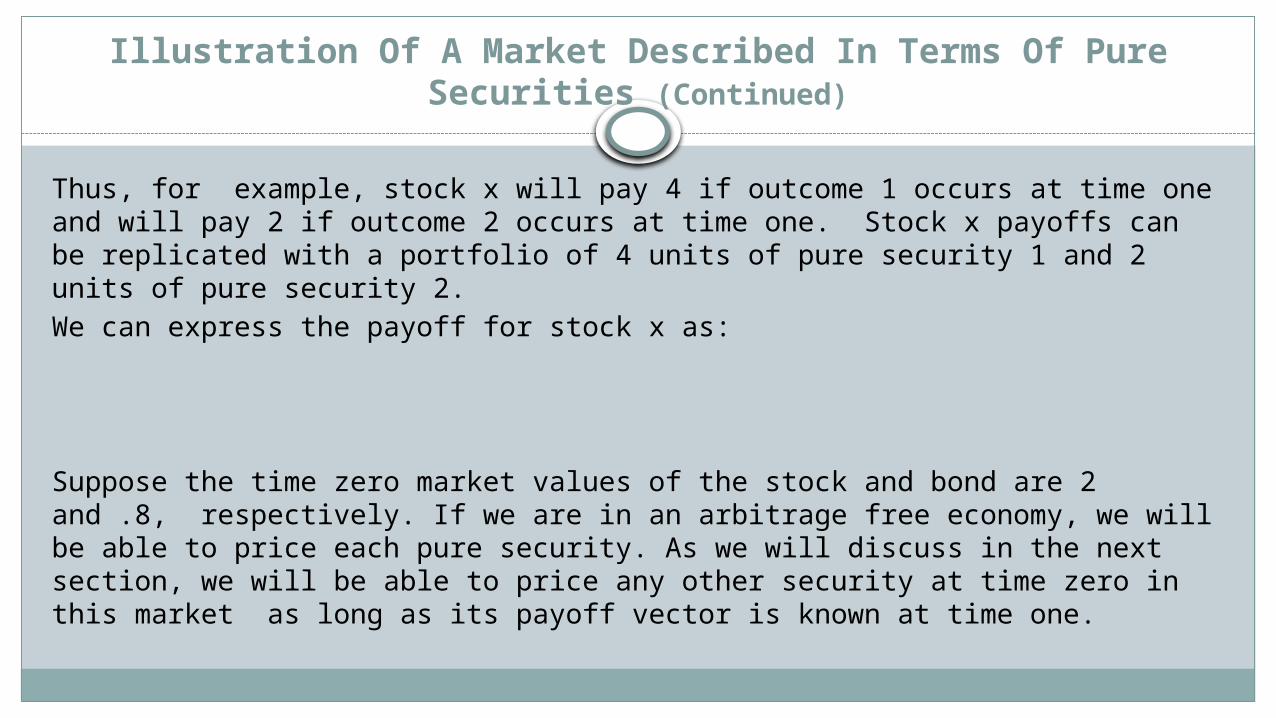
Illustration Of A Market Described In Terms Of Pure Securities (Continued)

Thus, for example, stock x will pay 4 if outcome 1 occurs at time one and will pay 2 if outcome 2 occurs at time one. Stock x payoffs can be replicated with a portfolio of 4 units of pure security 1 and 2 units of pure security 2. We can express the payoff for stock x as:

Suppose the time zero market values of the stock and bond are 2 and .8, respectively. If we are in an arbitrage free economy, we will be able to price each pure security. As we will discuss in the next section, we will be able to price any other security at time zero in this market as long as its payoff vector is known at time one.

Pricing Pure Securities

Suppose we are in a one time period n state economy with n already priced securities at time zero such that their payoff vectors at time one are linearly independent. We also assume that there are no opportunities for arbitrage. Then we will be able to obtain the time zero price for each of the n pure securities.

Pricing Pure Securities (Continued)

Let the matrix CF denote the payoffs of each of the n securities, where a given row j are the payoffs for security j for outcomes 1 through n. Let S denote the vector of prices of the n securities at time zero. Let ψ denote the vector of prices of the n pure securities. If there are no arbitrage opportunities, then the vector of pure securities must satisfy the equation:

The solution for the prices of the pure securities is:


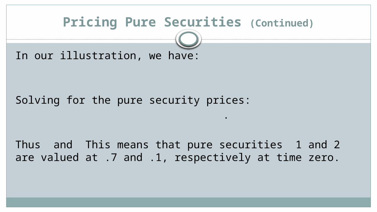
In our illustration, we have:

Solving for the pure security prices:

.

Thus and This means that pure securities 1 and 2 are valued at .7 and .1, respectively at time zero.


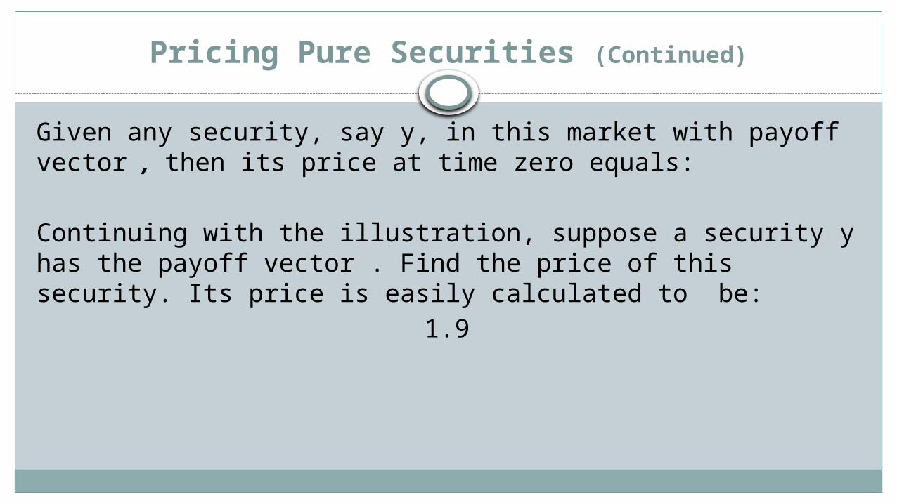
Given any security, say y, in this market with payoff vector , then its price at time zero equals:

Continuing with the illustration, suppose a security y has the payoff vector . Find the price of this security. Its price is easily calculated to be:

1.9

Synthetic Probabilities

If our analysis includes a riskless asset in the type of no arbitrage pricing model that we have been using in this section, every security in this no arbitrage market will have will have the same expected rate of return as the riskless bond under certain circumstances. An important feature of this type of pricing model in such a market is that it can be used to define “synthetic,” “hedging” or “risk-neutral” probabilities qi. These risk-neutral probabilities do not exist in any sort of realistic sense, nor are they assumed at the start of the modeling process. Instead, they are inferred from market prices of securities and interest rates.

Synthetic Probabilities (Continued)

These risk-neutral probabilities are essential in that they can be used to calculate the price of any security in the market so that the no arbitrage nature of the market is maintained. Risk neutral probabilities have the useful feature that they lead to expected values that are consistent with pricing by investors that are risk neutral, leading to the term risk neutral pricing. This is important because it means that we do not need to work with unobservable risk premiums when we value securities; in fact, we do not even need to know anything about any investors' risk preferences.


If payoffs for each of the pure securities e1, e2, …, en are the result of distinct outcomes, which together account for all possible outcomes (thus forming a sample space), then we can view the pricing model in terms of probabilities. The pure security prices are proportional to the market’s assessment of the relative likelihood that the outcomes that we number as 1, 2,… n, respectively, will occur.


Consider the previous example. The pure securities prices were calculated to be .7 and .1. This suggests that investors are willing to pay .7 for a security that pays 1 if and only if outcome 1 occurs, and .1 for a security that pays 1 if and only if outcome 2 occurs. If we assume that investors are risk neutral, this implies that they believe that outcome 1 is 7 times more likely to occur that outcome 2.

We create the riskless portfolio with payoff vector Observe that this portfolio pays off 1 regardless of which of the two outcomes occurs. Thus, this portfolio replicates a riskless bond that pays off 1 at time one.


In the illustration, the riskless bond was valued at .8 at time zero. Using our no arbitrage pricing equation, the bond price at time zero must satisfy the equation:

The pure security prices add up .8, which is less than 1. In this

example, as is usually the case, the ’s sum to a value less than 1 because of the time value of money.

Nevertheless, if we accept that should be proportional to the relative likelihood that outcome i will occur from the point of view of a risk neutral investor, then the probability that outcome i occurs is:


where ψi is the price of pure security i and ψj is the price of each of n pure securities j. In our illustration, synthetic probabilities are q1 = .7/.8 = .875 and q2 = .1/.8 = .125. These probabilities are referred to as synthetic probabilities because they are constructed from security prices rather than directly from investor assessments of physical probability.

Complete Markets And No Arbitrage Pricing

A complete market is one in which the payoffs for any security can be replicated by a portfolio of existing securities that have already been priced. We also assume that the market is frictionless, which means that there are no transactions costs associated with the purchase or sale of securities.

If, in addition, there are no arbitrage opportunities, then any security can be priced with the replicating portfolio of the already priced securities.

Suppose there are n possible outcomes (or states) in the market, which implies there are n possible payoffs for each security. Each security’s payoffs are then defined by a n dimensional payoff vector.

Complete Markets And No Arbitrage Pricing (Continued)

In a complete market with n possible outcomes, there must exist already priced securities so that their payoff vectors that span which represents all possible payoff vectors in the market. As we know from linear algebra, there must then exist a subset of n already priced securities with linearly independent payoff vectors. These n securities’ payoff vectors will form a basis for the payoff vector for every security in the market. If the market is also arbitrage free, every security can be priced in this market by the same methods we used to price bonds earlier in the chapter.

It can also be proved that the pricing of any particular security will be the same regardless of which set of n already priced securities with linearly independent payoff vectors one chooses to accomplish the pricing.

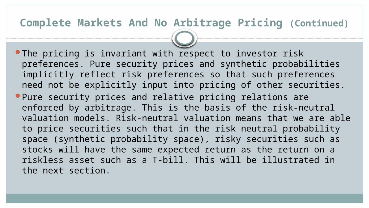
Complete Markets And No Arbitrage Pricing (Continued)

The pricing is invariant with respect to investor risk preferences. Pure security prices and synthetic probabilities implicitly reflect risk preferences so that such preferences need not be explicitly input into pricing of other securities.

Pure security prices and relative pricing relations are enforced by arbitrage. This is the basis of the risk-neutral valuation models. Risk-neutral valuation means that we are able to price securities such that in the risk neutral probability space (synthetic probability space), risky securities such as stocks will have the same expected return as the return on a riskless asset such as a T-bill. This will be illustrated in the next section.

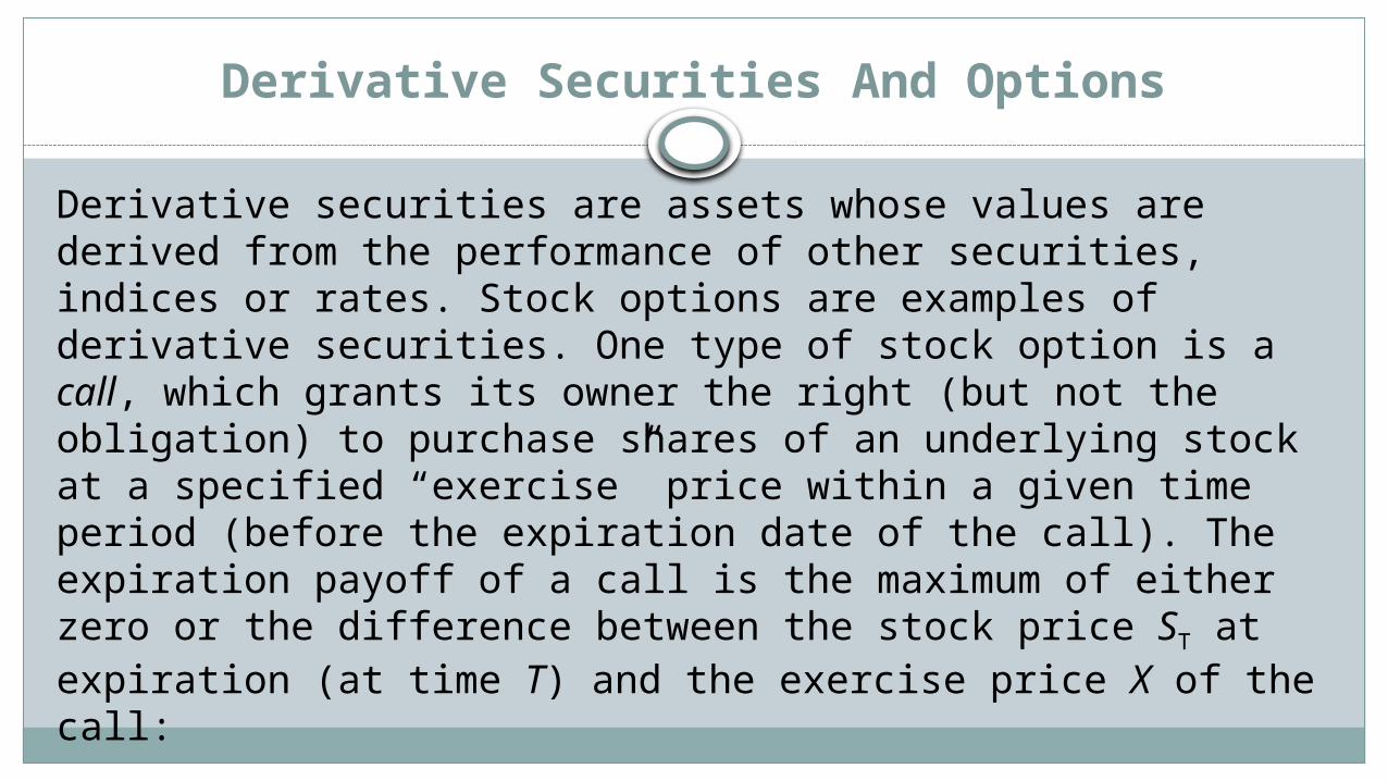
Derivative Securities And Options

Derivative securities are assets whose values are derived from the performance of other securities, indices or rates. Stock options are examples of derivative securities. One type of stock option is a call, which grants its owner the right (but not the obligation) to purchase shares of an underlying stock at a specified “exercise” price within a given time period (before the expiration date of the call). The expiration payoff of a call is the maximum of either zero or the difference between the stock price ST at expiration (at time T) and the exercise price X of the call:

cT = MAX[ST - X,0]

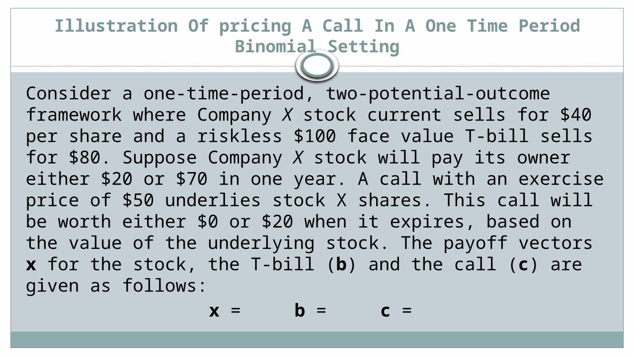
Illustration Of pricing A Call In A One Time Period Binomial Setting

Consider a one-time-period, two-potential-outcome framework where Company X stock current sells for $40 per share and a riskless $100 face value T-bill sells for $80. Suppose Company X stock will pay its owner either $20 or $70 in one year. A call with an exercise price of $50 underlies stock X shares. This call will be worth either $0 or $20 when it expires, based on the value of the underlying stock. The payoff vectors x for the stock, the T-bill (b) and the call (c) are given as follows:

x = b = c =

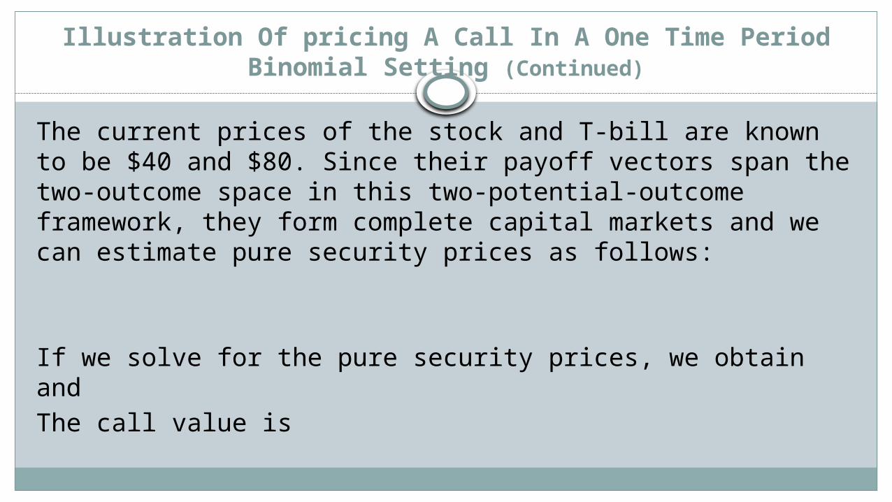
Illustration Of pricing A Call In A One Time Period Binomial Setting (Continued)

The current prices of the stock and T-bill are known to be $40 and $80. Since their payoff vectors span the two-outcome space in this two-potential-outcome framework, they form complete capital markets and we can estimate pure security prices as follows:

If we solve for the pure security prices, we obtain and The call value is


The risk-neutral probabilities (synthetic probabilities) are determined as follows:

With respect to the risk-neutral probabilities, the expected value of stock X is: E[X]=q1x1+q2x2 = .4×20 +.6×70 = 50, which gives an expected return of (50-40)/40 = 25%. The return on the riskless T-bill is: (100-80)/80 = 25%. The returns are equal, thus illustrating the risk-neutral nature of the arbitrage free pricing mechanism.


We can also use the concept of arbitrage to directly value the call. Since the call and bond are priced, and their payoff vectors of the stock and T-bill span the 2-outcome space, they form complete capital markets. Thus, a portfolio comprising the stock and T-bill can replicate the payoff structure of the call:

Solving for the portfolio positions gives:

Thus, the payoff structure of the call is replicated with buying .4 shares of the stock and shorting .08 units of the bond. This portfolio requires a net investment of .4×40-.08×80=$9.60, which must also be the value of the call.

Put-Call Parity

A put is an option that grants its owner the right to sell the underlying stock at a specified exercise price on or before its expiration date.

Consider a European put (European options can be exercised only at expiration) with value p0 and a European call with value c0 written on the same underlying stock currently priced at S0. Both options have exercise prices equal to X and expire at time T. The riskless return rate is r.

The payoff function of the call at expiration is cT = MAX[ST-X, 0] and the payoff function for the put is pT = MAX[X-ST, 0]. Observe that at expiration we have the relationship:

or equivalently:

Put-Call Parity (Continued)

At expiration time T, in an n outcome space at time T, the relationship would be expressed as a vector equation involving the possible payoffs:

where p is the put payoff vector, s is the vector prices of the stock, X is the exercise price expressed as a vector, and c is the call payoff vector.

In our previous illustration, assuming the put has the same time period and the same exercise price as the call, then at expiration we have the relationship:

Put-Call Parity (Continued)

The relationship between the put, stock price, exercise price, and call must hold for all times, including at time 0, except that we have to discount the exercise price by to obtain its value at time 0. Furthermore, at time 0, the values of these quantities are all known. Thus, we have the relationship:

In our previous illustration, if we assume the same time period and exercise price on a put, the value of the put would be:

Documents

Chapter 3 Discrete Time and State Models. Discount Functions