Embed Size (px)
Citation preview
Chapter 3: Delta Modulation
Digital Communication Systems 2012 R.Sokullu 1/45
CHAPTER 3
DELTA MODULATION
Chapter 3: Delta Modulation
Digital Communication Systems 2012 R.Sokullu 2/45
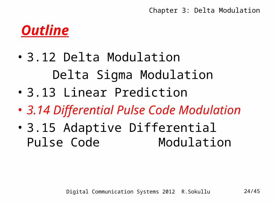
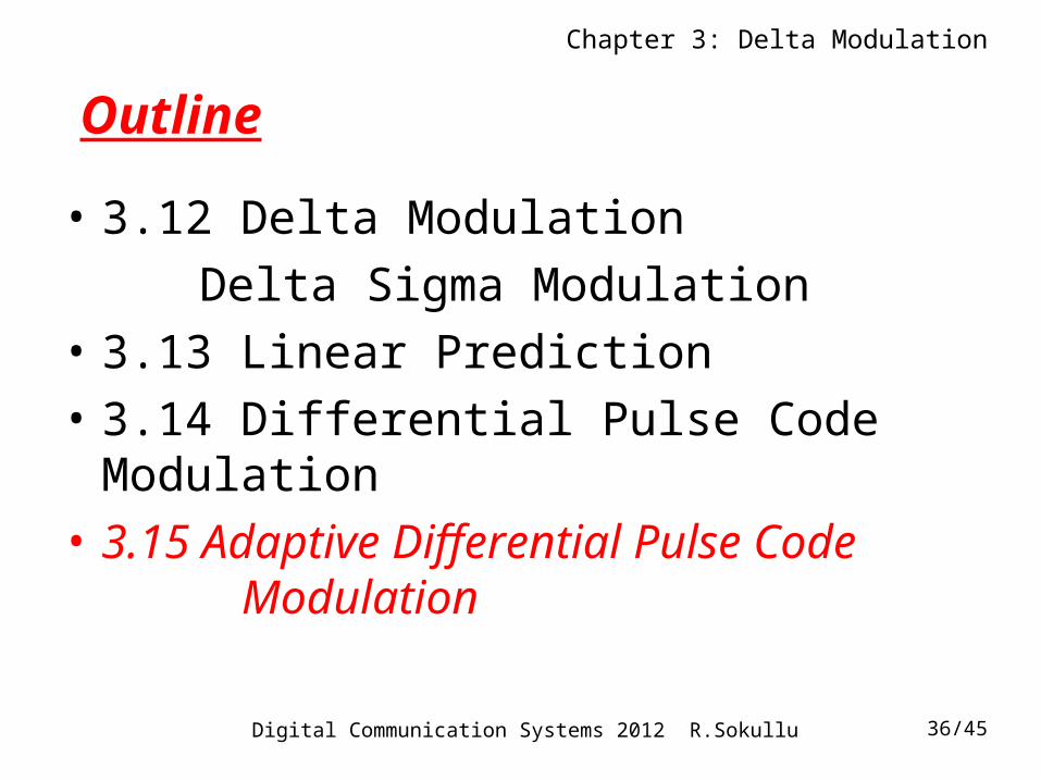
Outline
• 3.12 Delta Modulation
Delta Sigma Modulation
• 3.13 Linear Prediction
• 3.14 Differential Pulse Code Modulation
• 3.15 Adaptive Differential Pulse Code Modulation
Chapter 3: Delta Modulation
Digital Communication Systems 2012 R.Sokullu 3/45
3.12 Delta Modulation
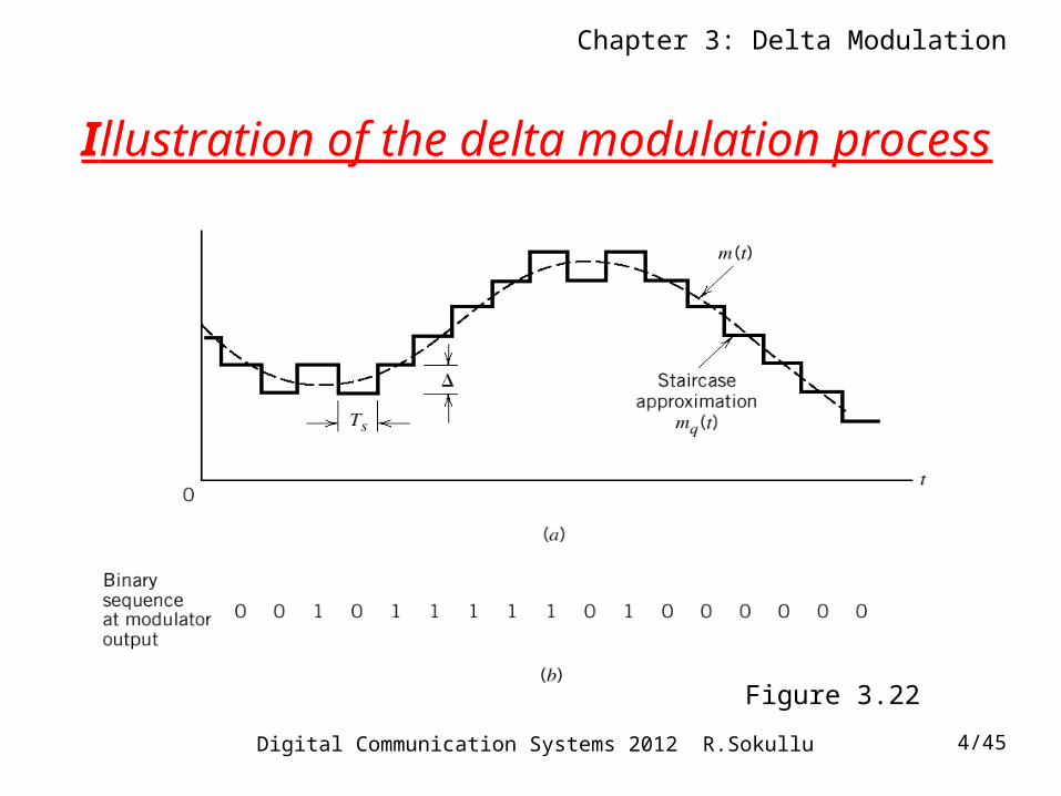
• Definition: Delta Modulation is a technique which provides a staircase approximation to an over-sampled version of the message signal (analog input).
• sampling is at a rate higher than the Nyquist rate – aims at increasing the correlation between adjacent samples; simplifies quantizing of the encoded signal
Chapter 3: Delta Modulation
Digital Communication Systems 2012 R.Sokullu 4/45
Illustration of the delta modulation process
Figure 3.22
Chapter 3: Delta Modulation
Digital Communication Systems 2012 R.Sokullu 5/45
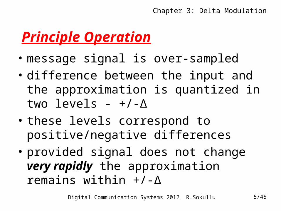
Principle Operation
• message signal is over-sampled
• difference between the input and the approximation is quantized in two levels - +/-Δ
• these levels correspond to positive/negative differences
• provided signal does not change very rapidly the approximation remains within +/-Δ
Chapter 3: Delta Modulation
Digital Communication Systems 2012 R.Sokullu 6/45
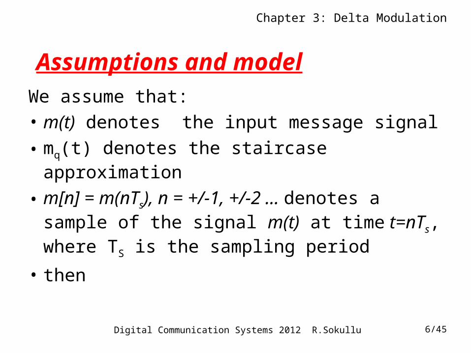
Assumptions and model
We assume that:
• m(t) denotes the input message signal
• mq(t) denotes the staircase approximation
• m[n] = m(nTs), n = +/-1, +/-2 … denotes a sample of the signal m(t) at time t=nTs, where TS is the sampling period
• then
Chapter 3: Delta Modulation
Digital Communication Systems 2012 R.Sokullu 7/45
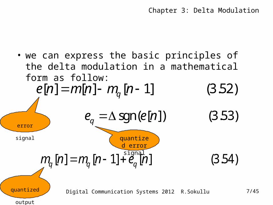
• we can express the basic principles of the delta modulation in a mathematical form as follow:
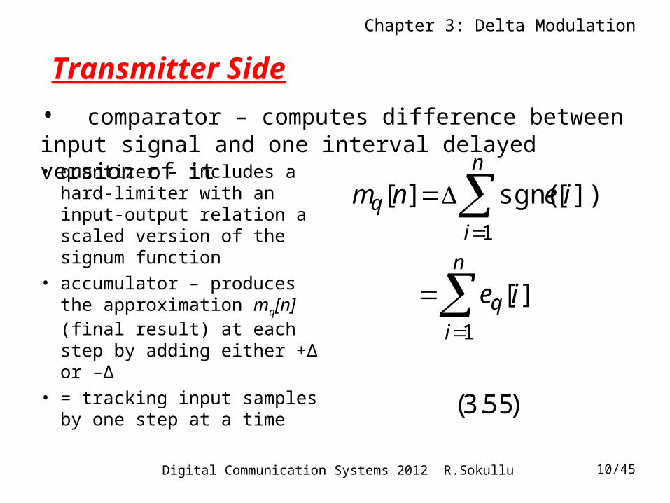
[ ] [ ] [ 1] (3.52)qe n m n m n
sgn( [ ]) (3.53)qe e n
[ ] [ 1] [ ] (3.54)q q qm n m n e n
error signal
quantized
output
quantized error signal
Chapter 3: Delta Modulation
Digital Communication Systems 2012 R.Sokullu 8/45
Pros and cons
• Main advantage – simplicity
• Sampled version of the message is applied to a modulator (comparator, quantizer, accumulator)
• delay in accumulator is “unit delay” = one sample period (z-1)
Chapter 3: Delta Modulation
Digital Communication Systems 2012 R.Sokullu 9/45
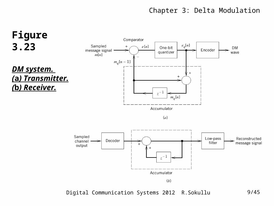
Figure 3.23
DM system. (a) Transmitter. (b) Receiver.
Chapter 3: Delta Modulation
Digital Communication Systems 2012 R.Sokullu 10/45
• quantizer – includes a hard-limiter with an input-output relation a scaled version of the signum function
• accumulator – produces the approximation mq[n] (final result) at each step by adding either +Δ or –Δ
• = tracking input samples by one step at a time
)55.3(
][
])[sgn(][
1
1
n
i
q
n
i
q
ie
ienm
• comparator – computes difference between input signal and one interval delayed version of it
Transmitter Side
Chapter 3: Delta Modulation
Digital Communication Systems 2012 R.Sokullu 11/45
Receiver Side
• decoder – creates the sequence of positive or negative pulses
• accumulator – creates the staircase approximation mq[n] similar to tx side
• out-of-band noise is cut off by low-pass filter (bandwidth equal to original message bandwidth)
Chapter 3: Delta Modulation
Digital Communication Systems 2012 R.Sokullu 12/45
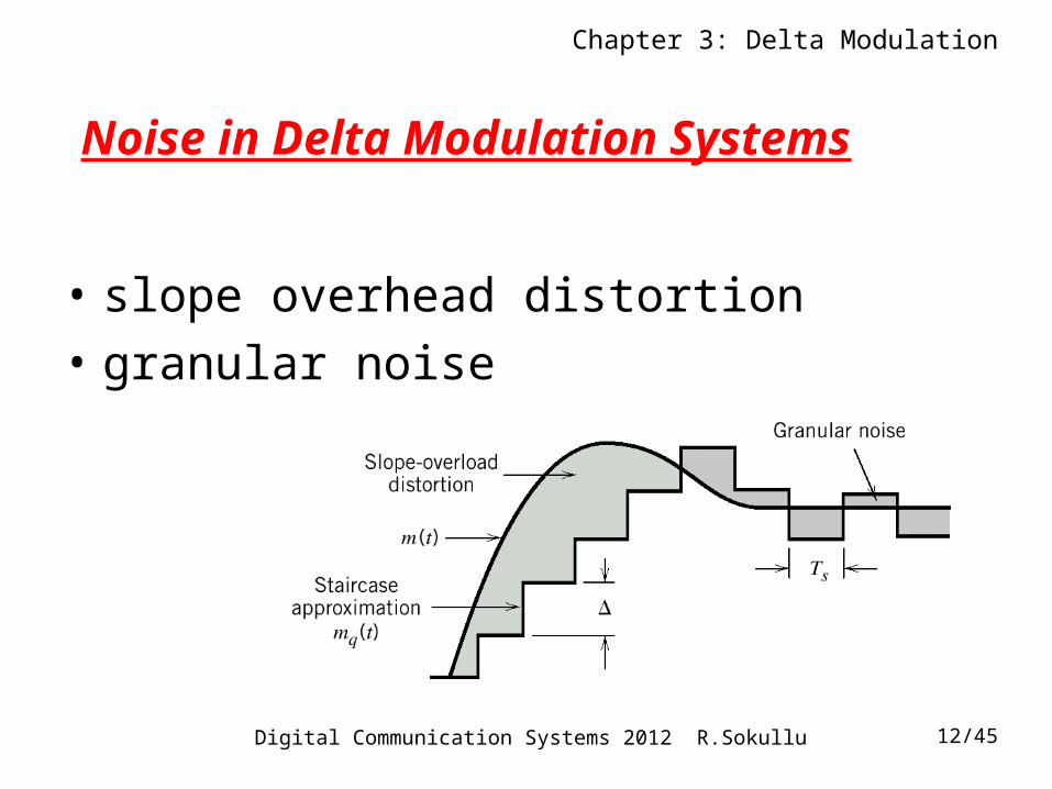
Noise in Delta Modulation Systems
• slope overhead distortion
• granular noise
Chapter 3: Delta Modulation
Digital Communication Systems 2012 R.Sokullu 13/45
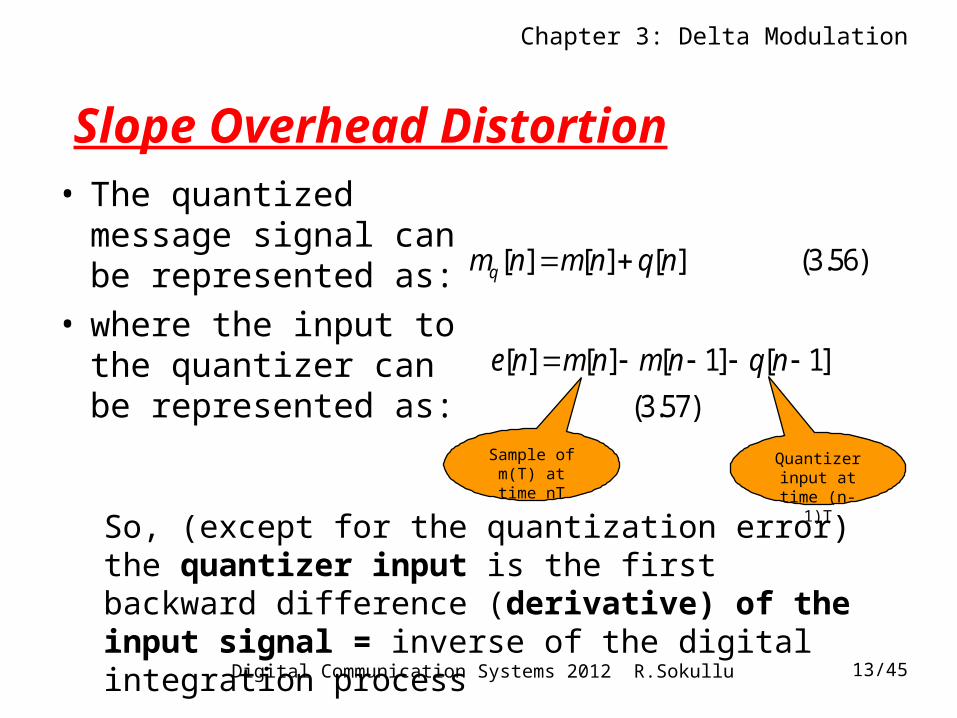
Slope Overhead Distortion• The quantized message
signal can be represented as:
• where the input to the quantizer can be represented as:
[ ] [ ] [ ] (3.56)qm n m n q n
[ ] [ ] [ 1] [ 1]
(3.57)
e n m n m n q n
So, (except for the quantization error) the quantizer input is the first backward difference (derivative) of the input signal = inverse of the digital integration process
Sample of m(T) at time nT
Quantizer input at time (n-1)T
Chapter 3: Delta Modulation
Digital Communication Systems 2012 R.Sokullu 14/45
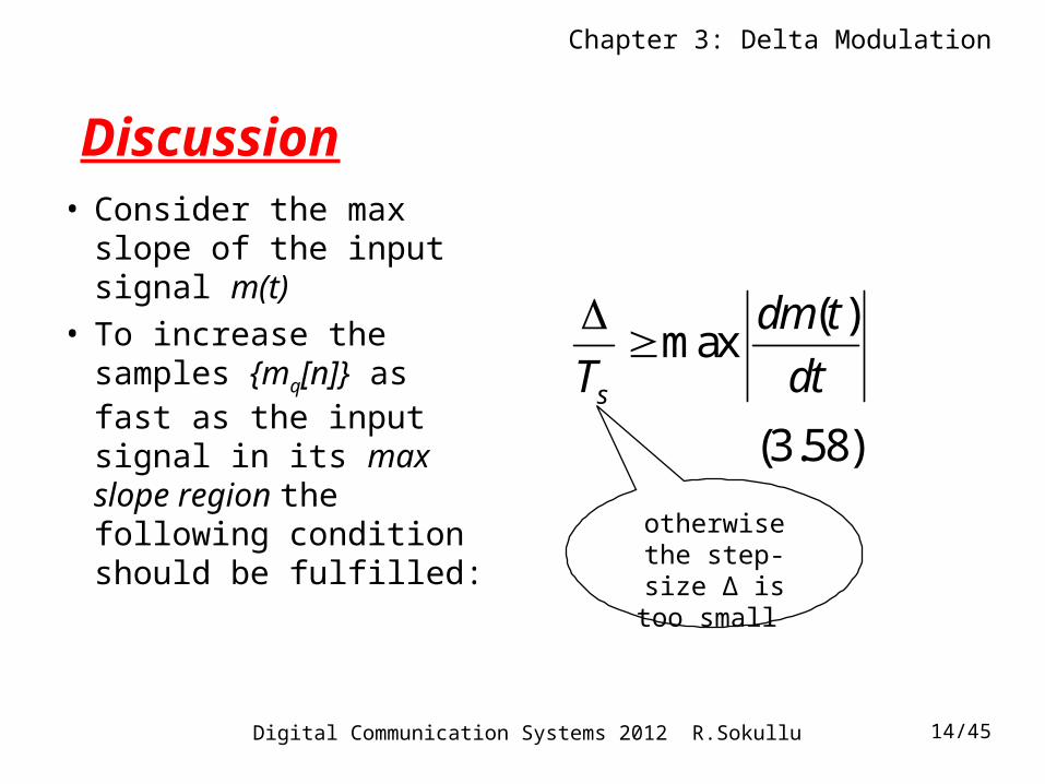
Discussion• Consider the max slope
of the input signal m(t)• To increase the samples
{mq[n]} as fast as the input signal in its max slope region the following condition should be fulfilled:
( )max
(3.58)s
dm t
T dt
otherwise the step-size Δ is too
small
Chapter 3: Delta Modulation
Digital Communication Systems 2012 R.Sokullu 15/45
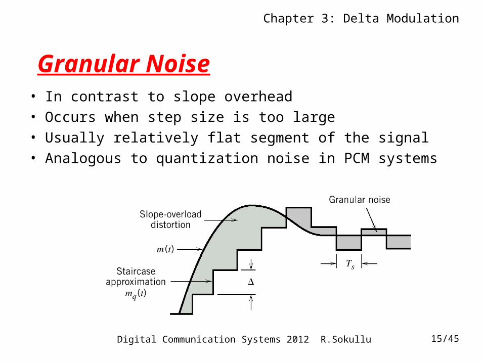
Granular Noise• In contrast to slope overhead
• Occurs when step size is too large
• Usually relatively flat segment of the signal
• Analogous to quantization noise in PCM systems
Chapter 3: Delta Modulation
Digital Communication Systems 2012 R.Sokullu 16/45
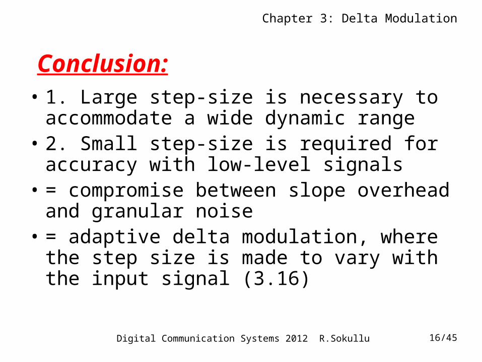
Conclusion:• 1. Large step-size is necessary to
accommodate a wide dynamic range• 2. Small step-size is required for accuracy with
low-level signals• = compromise between slope overhead and
granular noise• = adaptive delta modulation, where the step
size is made to vary with the input signal (3.16)
Chapter 3: Delta Modulation
Digital Communication Systems 2012 R.Sokullu 17/45
Outline
• 3.12 Delta Modulation
Delta Sigma Modulation
• 3.13 Linear Prediction
• 3.14 Differential Pulse Code Modulation
• 3.15 Adaptive Differential Pulse Code Modulation
Chapter 3: Delta Modulation
Digital Communication Systems 2012 R.Sokullu 18/45
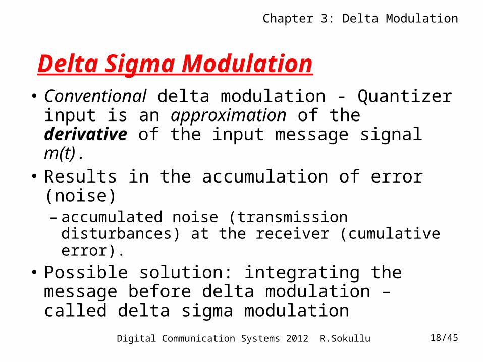
Delta Sigma Modulation• Conventional delta modulation - Quantizer
input is an approximation of the derivative of the input message signal m(t).
• Results in the accumulation of error (noise)– accumulated noise (transmission disturbances) at
the receiver (cumulative error).
• Possible solution: integrating the message before delta modulation – called delta sigma modulation
Chapter 3: Delta Modulation
Digital Communication Systems 2012 R.Sokullu 19/45
Remark 1:• The message signal is defined in its continuous
form – so pulse modulator contains a hard limiter and a pulse generator to produce a 1-bit encoded signal
• integration at the tx requires differentiation at the rx side.
• But: As in conventional DM the message has to be integrated at the final stage this eliminates the need of differentiation here.
Chapter 3: Delta Modulation
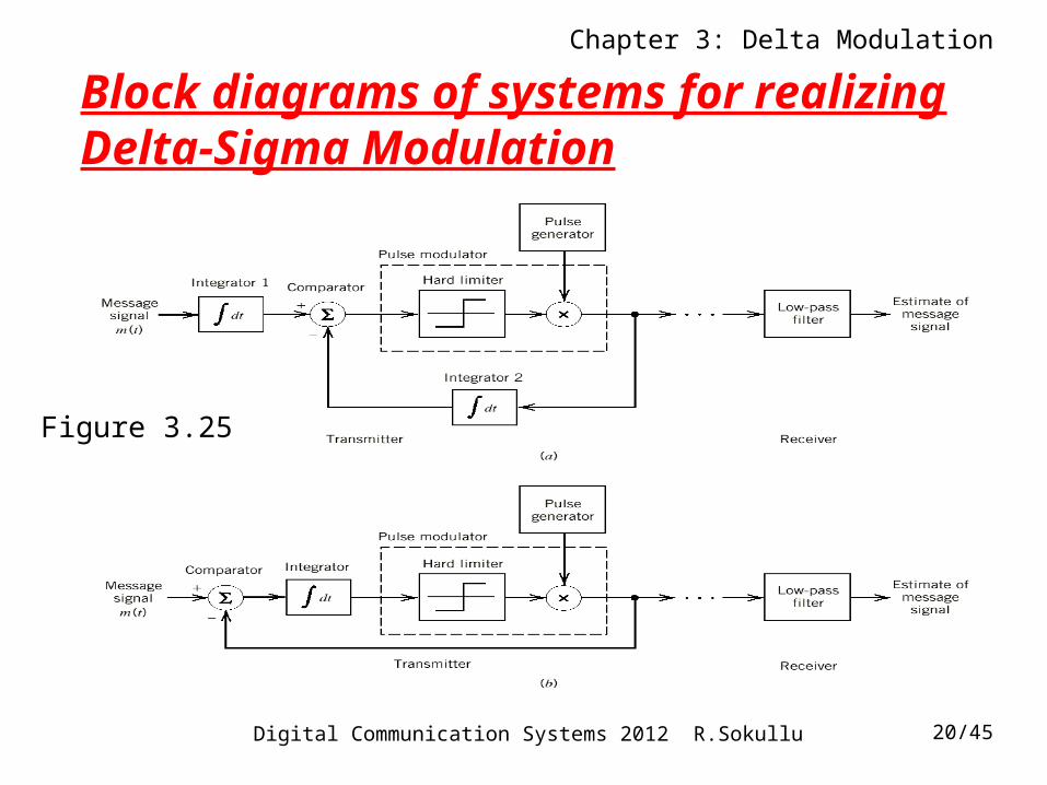
Digital Communication Systems 2012 R.Sokullu 20/45
Block diagrams of systems for realizing Delta-Sigma Modulation
Figure 3.25
Chapter 3: Delta Modulation
Digital Communication Systems 2012 R.Sokullu 21/45
Remark 2:
• Integration is a linear operation
• Int 1 and Int 2 can be combined in a single integrator placed after the comparator (previous slide – 3.25 b)
• Results in a simpler version of DSM scheme
Chapter 3: Delta Modulation
Digital Communication Systems 2012 R.Sokullu 22/45
Pros and cons for DSM• Simplicity of implementation both at the tx
and rx side• Requires sampling rate far in excess of the
Nyquist rate (PCM) – increase in transmission and channel bandwidth
• If bandwidth is at a premium we have to choose increased system complexity (additional signal processing) to achieve reduced bandwidth.
Chapter 3: Delta Modulation
Digital Communication Systems 2012 R.Sokullu 23/45
How does it work?
• Reading assignment:
• 3.13 Linear Prediction
(plus all that you are taught in the Signals and Systems – part II)
Chapter 3: Delta Modulation
Digital Communication Systems 2012 R.Sokullu 24/45
Outline
• 3.12 Delta Modulation
Delta Sigma Modulation
• 3.13 Linear Prediction
• 3.14 Differential Pulse Code Modulation
• 3.15 Adaptive Differential Pulse Code Modulation
Chapter 3: Delta Modulation
Digital Communication Systems 2012 R.Sokullu 25/45
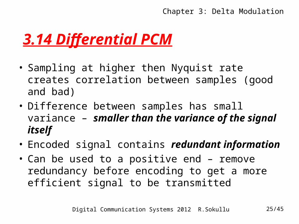
3.14 Differential PCM
• Sampling at higher then Nyquist rate creates correlation between samples (good and bad)
• Difference between samples has small variance – smaller than the variance of the signal itself
• Encoded signal contains redundant information• Can be used to a positive end – remove redundancy
before encoding to get a more efficient signal to be transmitted
Chapter 3: Delta Modulation
Digital Communication Systems 2012 R.Sokullu 26/45
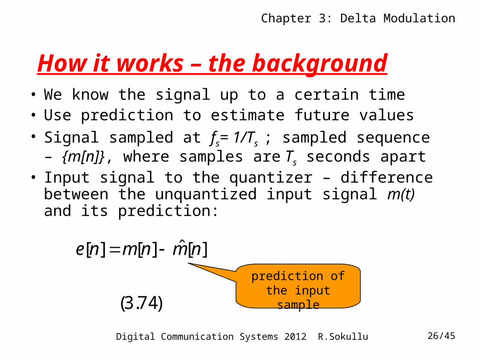
How it works – the background• We know the signal up to a certain time• Use prediction to estimate future values• Signal sampled at fs= 1/Ts ; sampled sequence –
{m[n]}, where samples are Ts seconds apart• Input signal to the quantizer – difference between
the unquantized input signal m(t) and its prediction:
)74.3(
][ˆ][][ nmnmne prediction of the
input sample
Chapter 3: Delta Modulation
Digital Communication Systems 2012 R.Sokullu 27/45
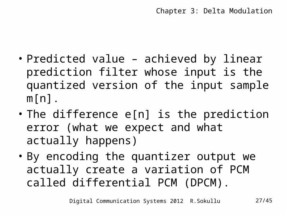
• Predicted value – achieved by linear prediction filter whose input is the quantized version of the input sample m[n].
• The difference e[n] is the prediction error (what we expect and what actually happens)
• By encoding the quantizer output we actually create a variation of PCM called differential PCM (DPCM).
Chapter 3: Delta Modulation
Digital Communication Systems 2012 R.Sokullu 28/45
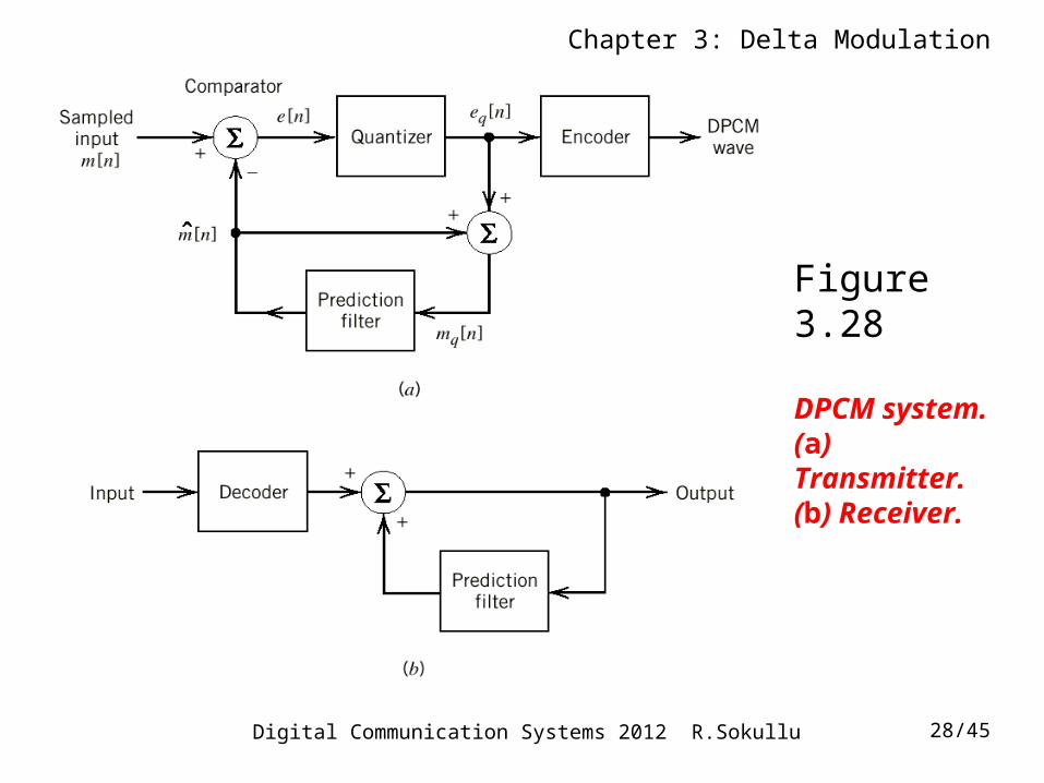
Figure 3.28
DPCM system. (a) Transmitter. (b) Receiver.
Chapter 3: Delta Modulation
Digital Communication Systems 2012 R.Sokullu 29/45
Details:• Block scheme is very similar to DM• quantizer input
ˆ[ ] [ ] [ ] (3.74)e n m n m n
[ ] [ ] [ ] (3.75)qe n e n q n
ˆ[ ] [ ] [ ] (3.76)q qm n m n e n
• quantizer output may be expressed as:
• prediction filter output may be expressed as:
Chapter 3: Delta Modulation
Digital Communication Systems 2012 R.Sokullu 30/45
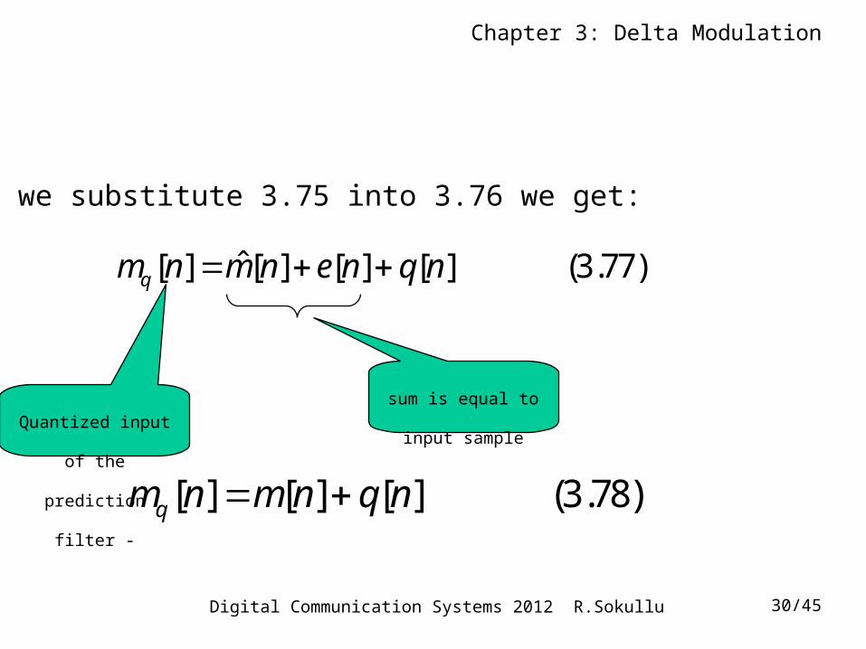
ˆ[ ] [ ] [ ] [ ] (3.77)qm n m n e n q n
If we substitute 3.75 into 3.76 we get:
sum is equal to input
sample
[ ] [ ] [ ] (3.78)qm n m n q n
Quantized input of the
prediction filter -
Chapter 3: Delta Modulation
Digital Communication Systems 2012 R.Sokullu 31/45
Details – cont’d
• mq[n] is the quantized version of the input sample m[n]• so, irrespective of the properties of the prediction filter the
quantized sample mq[n] at the prediction filter input differs from the original sample m[n] with the quantization error q[n].
• If the prediction filter is good, the variance of the prediction error e[n] will be smaller than the variance of m[n]
• This means that if we make a very good prediction filter (adjust the number of levels) it will be possible to produce a quantization error with a smaller variance than if the input sample m[n] is quantized directly as in standard PCM
Chapter 3: Delta Modulation
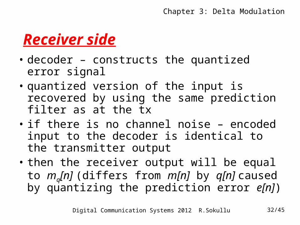
Digital Communication Systems 2012 R.Sokullu 32/45
Receiver side• decoder – constructs the quantized error signal • quantized version of the input is recovered by
using the same prediction filter as at the tx• if there is no channel noise – encoded input to
the decoder is identical to the transmitter output
• then the receiver output will be equal to mq[n] (differs from m[n] by q[n] caused by quantizing the prediction error e[n])
Chapter 3: Delta Modulation
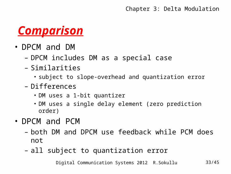
Digital Communication Systems 2012 R.Sokullu 33/45
Comparison• DPCM and DM
– DPCM includes DM as a special case
– Similarities• subject to slope-overhead and quantization error
– Differences• DM uses a 1-bit quantizer
• DM uses a single delay element (zero prediction order)
• DPCM and PCM– both DM and DPCM use feedback while PCM does not
– all subject to quantization error
Chapter 3: Delta Modulation
Digital Communication Systems 2012 R.Sokullu 34/45
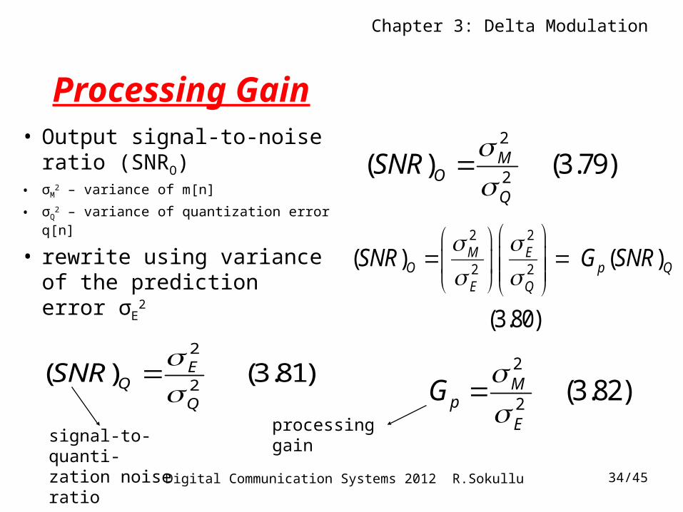
Processing Gain• Output signal-to-noise
ratio (SNRO)• σM
2 – variance of m[n]
• σQ2 – variance of quantization error q[n]
• rewrite using variance of the prediction error σE
2
2
2( ) (3.79)M
OQ
SNR
2 2
2 2( ) ( )
(3.80)
M EO p Q
E Q
SNR G SNR
2
2( ) (3.81)E
SNR
2
2(3.82)M
pE
G
signal-to-quanti-zation noise ratio
processing gain
Chapter 3: Delta Modulation
Digital Communication Systems 2012 R.Sokullu 35/45
• The processing gain Gp when greater than unity represents the signal-to-noise ratio that is due to the differential quantization scheme.
• For a given input message signal σM is fixed, so the smaller the σE the greater the Gp.
• This is the design objective of the prediction filter• For voice signals – optimal main advantage of DPCM
over PCM is b/n 4-11 dB• Advantage expressed in terms of bit rate (bits)
– 1 bit =6 dB of quantization noise (Table 3.35, p 198)– So for fixed SNR, sampling rate 8 kHz – DCPM provides
saving of 8-16 kb/s (1 -2 bits per sample) PCM
Chapter 3: Delta Modulation
Digital Communication Systems 2012 R.Sokullu 36/45
Outline
• 3.12 Delta Modulation
Delta Sigma Modulation
• 3.13 Linear Prediction
• 3.14 Differential Pulse Code Modulation
• 3.15 Adaptive Differential Pulse Code Modulation
Chapter 3: Delta Modulation
Digital Communication Systems 2012 R.Sokullu 37/45
3.15 Adaptive Differential PCM • PCM for speech coding of 64 kb/s requires high
channel bandwidth• some applications (secure transmission over radio
channel – low capacity)• requires speech coding at low bit rates but preserving
acceptable fidelity (not 64 kb/s PCM but 32, 16, 8 etc)
• possible using special coders that utilize statistical characteristics of speech signals and properties of hearing
Chapter 3: Delta Modulation
Digital Communication Systems 2012 R.Sokullu 38/45
Design Objectives• 1. Remove redundancies from speech signals• 2. Assign available bits to encode non-redundant
parts of speech signal in an efficient way• Standard PCM is at 64 kb/s – can be reduced to 32,
16, 8 or even 4 kb/s• Price = proportionally increased complexity
– For same speech quality but Half the bit rate - Computational complexity is an order of magnitude higher
Chapter 3: Delta Modulation
Digital Communication Systems 2012 R.Sokullu 39/45
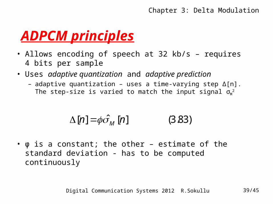
ADPCM principles• Allows encoding of speech at 32 kb/s – requires 4 bits per
sample
• Uses adaptive quantization and adaptive prediction– adaptive quantization – uses a time-varying step Δ[n]. The step-
size is varied to match the input signal σM2
• φ is a constant; the other – estimate of the standard deviation - has to be computed continuously
ˆ[ ] [ ] (3.83)Mn n
Chapter 3: Delta Modulation
Digital Communication Systems 2012 R.Sokullu 40/45
• Two possibilities:– adaptive quantization with forward estimation
(AQF) – uses unquantized samples of the input signal to derive forward estimates of σM[n]; requires a buffer to store samples for a certain learning period; incurs delay (~ 16 ms for speech)
– adaptive quantization with backward estimation (AQB) – uses samples of the quantizer output to derive backwards estimates of σM[n]
Chapter 3: Delta Modulation
Digital Communication Systems 2012 R.Sokullu 41/45
• Adaptive prediction in ADPCM– adaptive prediction with forward estimation
(APF); uses unqunatized samples of the input signal to calculate prediction coefficients; disadvantages similar to AQF
– adaptive prediction with backward estimation (APB); uses samples of the quantizer output and the prediction error to compute predictor coefficients; logic for adaptive prediction – algorithm for updating predictor coefficients
Chapter 3: Delta Modulation
Digital Communication Systems 2012 R.Sokullu 42/45
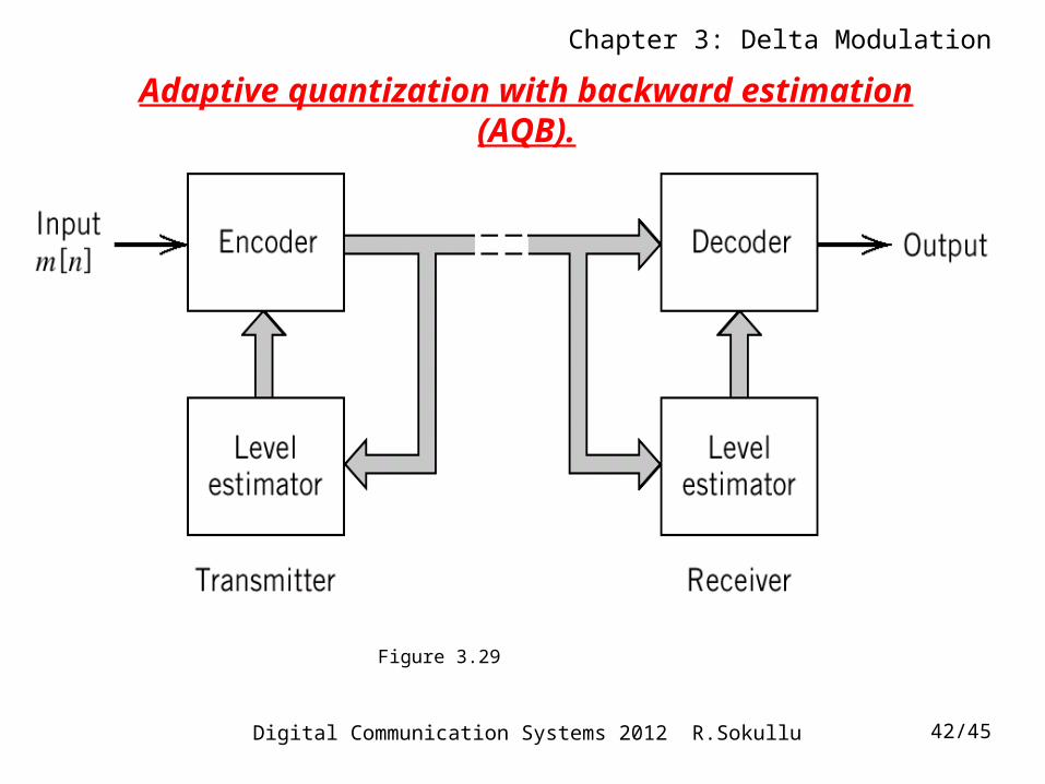
Figure 3.29
Adaptive quantization with backward estimation (AQB).
Chapter 3: Delta Modulation
Digital Communication Systems 2012 R.Sokullu 43/45
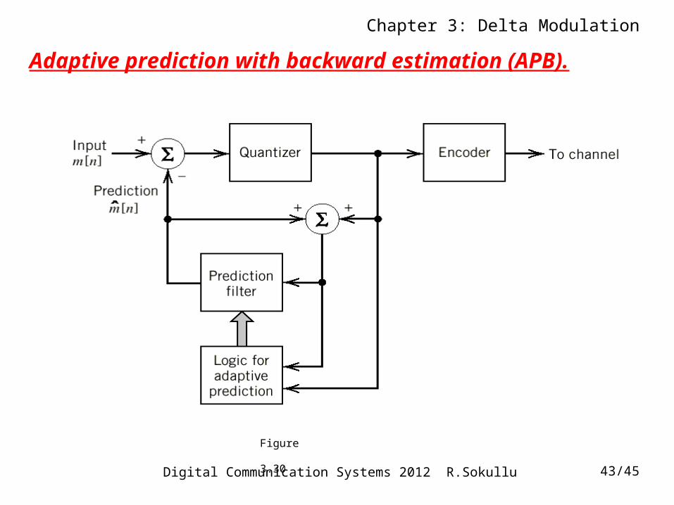
Adaptive prediction with backward estimation (APB).
Figure 3.30
Chapter 3: Delta Modulation
Digital Communication Systems 2012 R.Sokullu 44/44
Conclusion:
• PCM at 64 kb/s and ADPCM at 32 kb/s are internationally accepted standards for voice coding and decoding.