Embed Size (px)
Citation preview
44
Chapter 3: Classical Variational Methods and the
Finite Element Method
3.1 Introduction
Deriving the governing dynamics of physical processes is a complicated task in itself;
finding exact solutions to the governing partial differential equations is usually even more
formidable. When trying to solve such equations, approximate methods of analysis
provide a convenient, alternative method for finding solutions. Two such methods, the
Rayleigh-Ritz method and the Galerkin method, are typically used in the literature and
are referred to as classical variational methods.
According to Reddy (1993), when solving a differential equation by a variational method,
the equation is first put into a weighted-integral form, and then the approximate solution
within the domain of interest is assumed to be a linear combination )(∑i iic φ of
appropriately chosen approximation functions iφ and undetermined coefficients, ci . The
coefficients ci are determined such that the integral statement of the original system
dynamics is satisfied. Various variational methods, like Rayleigh-Ritz and Galerkin,
differ in the choice of integral form, weighting functions, and / or approximating
functions. Classical variational methods suffer from the disadvantage of the difficulty
associated with proper construction of the approximating functions for arbitrary domains.
The finite element method overcomes the disadvantages associated with the classical
variational methods via a systematic procedure for the derivation of the approximating
functions over subregions of the domain. As outlined by Reddy (1993), there are three
main features of the finite element method that give it superiority over the classical
variational methods. First, extremely complex domains are able to be broken down into a
collection of geometrically simple subdomains (hence the name finite elements).
Secondly, over the domain of each finite element, the approximation functions are
derived under the assumption that continuous functions can be well-approximated as a
45
linear combination of algebraic polynomials. Finally, the undetermined coefficients are
obtained by satisfying the governing equations over each element.
The goal of this chapter is to introduce some key concepts and definitions that apply to all
variational methods. Comparisons will be made between the Rayleigh-Ritz, Galerkin,
and finite element methods. Such comparisons will be highlighted through representative
problems for each. In the end, the benefits of the finite element method will be apparent.
3.2 Defining the Strong, Weak, and Weighted-Integral Forms
Most dynamical equations, when initially derived, are stated in their strong form. The
strong form for most mechanical systems consists of the partial differential equation
governing the system dynamics, the associated boundary conditions, and the initial
conditions for the problem, and can be thought of as the equation of motion derived using
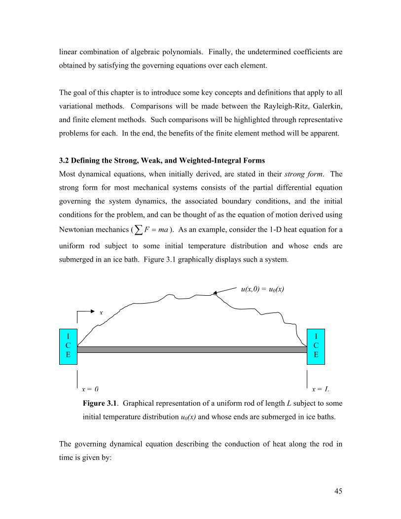
Newtonian mechanics (∑ = maF ). As an example, consider the 1-D heat equation for a
uniform rod subject to some initial temperature distribution and whose ends are
submerged in an ice bath. Figure 3.1 graphically displays such a system.
Figure 3.1. Graphical representation of a uniform rod of length L subject to some
initial temperature distribution u0(x) and whose ends are submerged in ice baths.
The governing dynamical equation describing the conduction of heat along the rod in
time is given by:
x = 0 x = L
ICE
ICE
u(x,0) = u0(x)
x
46
Lxfort
txux
txux
≤≤∂
∂=
∂∂
∂∂ 0),(),(2α (3.1)
subject to the initial temperature distribution
)()0,( 0 xuxu = (3.2)
and constrained by the following boundary conditions imposed by the ice baths:
0),(),0( == tLutu . (3.3)
The term 2α in Equation 3.1 is known as the thermal diffusivity of the rod and is defined
as
sρκα =2 , (3.4)
where κ is the thermal conductivity, ρ is the density, and s is the specific heat of the rod.
Equations 3.1-3.3 combine to define the strong form of the governing dynamics.
Physically, Equations 3.1-3.3 state that the heat flux is proportional to the temperature
gradient along the rod. The boundary conditions (Equation 3.3) are said to be
homogeneous since they are specified as being equal to zero on both ends of the rod. Had
the problem been defined with non-zero terms at each end, the boundary conditions
would be referred to as non-homogeneous.
Without actually solving Equation 3.1, we know that the solution, u(x,t), to the problem
will require two spatial derivatives, and it will have to satisfy the homogeneous boundary
conditions while being subject to an initial temperature distribution. Thus, in more
general terms, the strong solution to Equation 3.1 satisfies the differential equation and
47
boundary conditions exactly and must be as smooth (number of continuous derivatives)
as required by the differential equation. The fact that the strong solution must be as
smooth as required by the strong form of the differential equation is an immediate
downfall of the strong form. If the system under analysis consists of varying geometry or
material properties, then discontinuous functions will enter into the equations of motion
and the issue of differentiability can become immediately apparent. To avoid such
difficulties, we can change the strong form of the governing dynamics into a weak or
weighted-integral formulation.
If the weak form to a differential equation exists, then we can arrive at it through a series
of steps. First, for convenience, rewrite Equation 3.1 in a more compact form, namely
[ ] txx uu =2α , (3.5)
where the subscripts x and t refer to spatial and temporal partial derivatives, respectively.
Next, move all the expressions of the differential equation to one side, multiply through
the entire equation by an arbitrary function g, called the weight or test function, and
integrate over the domain Ω = [0, L] of the system:
[ ]( ) 00
2 =∫ +−L
txx dxuug α . (3.6)
Reddy (1993) refers to Equation 3.6 as the weighted-integral or weighted-residual
statement, and it is equivalent to the original system dynamics, Equation 3.1. Another
way of stating Equation 3.6 is when the solution u(x,t) is exact, the solution to Equation
3.6 is trivial. But, when we put an approximation in for u(x,t), there will be a non-zero
value left in the parenthetical of Equation 6. “Mathematically, [Equation 3.6] is a
statement that the error in the differential equation (due to the approximation of the
solution) is zero in the weighted-integral sense” (Reddy, 1993).
48
Since we are seeking an approximation to the dynamics given by Equation 3.1, the
weighted-integral form gives us a means to obtain N linearly independent equations to
solve for the coefficients ci in the approximation
∑=
=≈N
iii
N xtctxutxu1
)()(),(),( φ . (3.7)
Note that the weighted-integral form of the dynamic equation is not subject to any
boundary conditions. The boundary conditions will come into play subsequently.
The next step in deriving the weak form of the dynamics requires integrating Equation
3.6 by parts. Doing so yields:
( ) [ ] 002
0
2 =−+∫L
x
L
txx gudxgugu αα . (3.8)
Firstly, it is important to recognize that the process of integrating the weighted-integral
equation (Equation 3.6) by parts, the differentiation required by the strong form of the
dependent variable, u, is now distributed onto the test function, g. This is an important
characteristic of the weak form of the equation, as this step now requires weaker, that is,
less, continuity of the dependent variable u. Secondly, notice that because we have
integrated Equation 3.6 by parts, Equation 3.8 consequently contains two types of terms:
integral terms and boundary terms. Another advantage of the weak form of the equation
is that the natural boundary conditions are already included in the weak form, and
“therefore the approximate solution UN is required to satisfy only the essential [or
geometric] boundary conditions of the problem” (Reddy, 1993). In the heat conduction
example, the essential boundary conditions are given by Equation 3.3, as they are
specified directly for the dependent variable u.
The final step in the weak formulation is to impose the actual boundary conditions of the
problem under consideration. Now, we wish the test function, g, to vanish at the
49
boundary points where the essential boundary conditions are defined. As explained by
Reddy (1993), the reasoning behind this step is that the test function has the meaning of a
virtual change (hence the term variation) of the primary variable, which in the case of the
heat conduction problem is u. Since u is known exactly at both ends of the rod, as they
are dipped in an ice bath, there cannot be any variation at the boundaries. Hence, we
need to require that the test function g vanish at these points. Therefore, we have
0)()0( == Lgg , (3.9)
in line with the essential boundary conditions specified by Equation 3.3. Imposing these
requirements on the test function gives us the reduced expression
( ) 00
2 =+∫L
txx dxguguα , (3.10)
which is the weak or variational form of the differential equation. The terms “weak” and
“variational” can be used interchangeably. Also, note that the difference between the
weak form and the weighted-integral form is that the weak form consists of the weighted-
integral form of the differential equation and, unlike the weighted-integral form, also
includes the specified natural boundary conditions of the problem.
In short summary, the main steps in arriving at the weak form of a differential equation
are as follows. First, move all of the expressions of the differential equation to one side.
Then, multiply through by a test function and integrate over the domain of the problem.
The resulting equation is called the weighted-integral form. Next, integrate the weighted-
integral form by parts to capture the natural boundary conditions and to expose the
essential boundary conditions. Finally, make sure that the test function satisfies the
homogeneous boundary terms where the essential boundary conditions are specified by
the problem. The resulting form is the weak or variational form of the original
differential equation. The main benefits of the weak form are that it requires weaker
smoothness of the dependent variable, and that the natural and essential boundary
50
conditions of the problem are methodically exposed because of the steps involved in the
formulation. Next, we will explore the differences between the Rayleigh-Ritz, Galerkin,
and finite element variational methods of approximation.
3.3 The Variational Methods of Approximation
This section will explore three different variational methods of approximation for solving
differential equations. Two classical variational methods, the Rayleigh-Ritz and Galerkin
methods, will be compared to the finite element method. All three methods are based on
either the weighted-integral form or the weak form of the governing dynamical equation,
and all three “seek an approximate solution in the form of a linear combination of
suitable approximation functions, iφ , and undetermined parameters, ci: ∑i iic φ ” (Reddy,
1993). However, the choice of the approximation functions used in each method will
highlight significant differences between each and emphasize the benefits of using the
finite element method.
3.3.1 The Rayleigh-Ritz Method
Before delving into the Rayleigh-Ritz method, a short historical perspective (summarized
from Meirovitch (1997)) is in order. The method was first used by Lord Rayleigh in
1870 (Gould, 1995) to solve the vibration problem of organ pipes closed on one end and
open at the other. However, the approach did not receive much recognition by the
scientific community. Nearly 40 years later, due to the publication of two papers by Ritz,
the method came to be called the Ritz method. To recognize the contributions of both
men, the theory was later renamed the Rayleigh-Ritz method. Leissa (2005) provides an
intriguing historical perspective on the controversy surrounding the development of this
methodology and its name.
As previously stated, the Rayleigh-Ritz method is based on the weak form of the
governing dynamics. It is important to note that the Rayleigh-Ritz method is only
applicable to self-adjoint problems. The choice of the test functions in formulating the
weak form is restricted to the approximation functions, namely:
51
jg φ= . (3.11)
Further, the test functions and approximation functions must be defined on the entire
domain of the problem. Although such a requirement seems trivial for problems like the
1-D heat conduction problem, it becomes a tremendous difficulty when applied in 2-D as
there isn’t a cookbook-type approach for finding admissible approximation functions. In
approximating the solution to the 1-D heat conduction example, we first start with the
weak form of the governing differential equation, Equation 3.10. For thoroughness, let’s
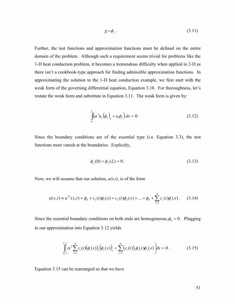
restate the weak form and substitute in Equation 3.11. The weak form is given by:
( )( ) 00
2 =+∫L
jtxjx dxuu φφα . (3.12)
Since the boundary conditions are of the essential type (i.e. Equation 3.3), the test
functions must vanish at the boundaries. Explicitly,
0)()0( == Ljj φφ . (3.13)
Now, we will assume that our solution, u(x,t), is of the form
∑=
+=+++=≈N
iii
N xtcxtcxtctxutxu1
022110 )()(...)()()()(),(),( φφφφφ . (3.14)
Since the essential boundary conditions on both ends are homogeneous, 00 =φ . Plugging
in our approximation into Equation 3.12 yields
( ) ( ) ( ) 0)()()()()()(0 11
2 =
+∫ ∑∑
==
L
j
N
iitixj
N
ixii dxxxtcxxtc φφφφα . (3.15)
Equation 3.15 can be rearranged so that we have
52
( ) ( ) ( )∫∑∫∑==
−=L
xjxi
N
ii
L
ji
N
iti dxxxtcdxxxtc
01
2
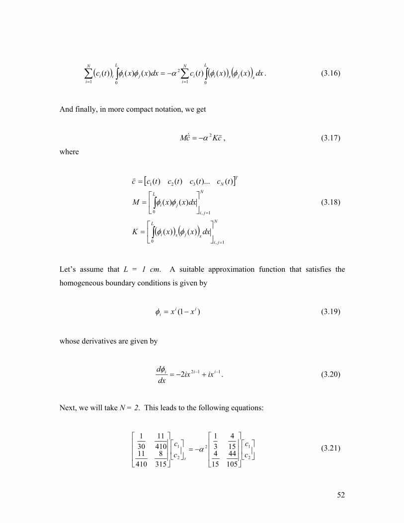
01)()()()()()( φφαφφ . (3.16)
And finally, in more compact notation, we get
cKcM v&v 2α−= , (3.17)
where
[ ]
( ) ( )N
ji
L
xjxi
N
ji
L
ji
TN
dxxxK
dxxxM
tctctctcc
1,0
1,0
321
)()(
)()(
)()...()()(
=
=
=
=
=
∫
∫
φφ
φφ
v
(3.18)
Let’s assume that L = 1 cm. A suitable approximation function that satisfies the
homogeneous boundary conditions is given by
)1( iii xx −=φ (3.19)
whose derivatives are given by
1122 −− +−= iii ixixdxdφ
. (3.20)
Next, we will take N = 2. This leads to the following equations:
−=
2
12
2
1
10544
154
154
31
3158
41011
41011
301
cc
cc
t
α (3.21)
53
For example purposes, let us also assume α2 = 1 cm2/s. Equation 3.21 then becomes
−=
2
1
2
1
10544
154
154
31
3158
41011
41011
301
cc
cc
t
. (3.22)
Next, we need to project our initial condition into the approximate domain, as well. Let’s
assume that our initial temperature distribution is given by:
( )xxu πsin)0,( = . (3.23)
Then, following the construction of the weak form, we have
∫∫==
=1
0
1
0
)()0,()()0,(L
j
L
jN dxxxudxxxu φφ . (3.24)
Plugging in our approximation, we have:
∫∫∑ ==
1
0
1
0 1)()0,()()()0( dxxxudxxxc jj
N
iii φφφ . (3.25)
Substituting in our shorthand notation from Equation 3.18 and our initial condition we get
( )∫=1
0
)(sin)0( dxxxcM jφπv . (3.26)
Finally, we can solve for the coefficients cv by solving
54
( )N
j
j dxxxMc1
1
0
1 )(sin)0(=
−
= ∫ φπv . (3.27)
Again, under the assumption that L = 1 cm and α2 = 1 cm2/s, we get the following initial
condition vector of coefficients:
−
=7034.0436.4
)0(cv . (3.28)
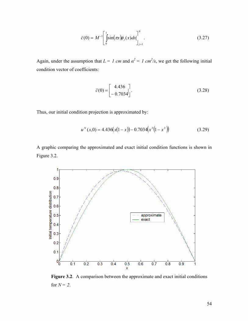
Thus, our initial condition projection is approximated by:
( )( ) ( )( )22 17034.01436.4)0,( xxxxxu N −−−= (3.29)
A graphic comparing the approximated and exact initial condition functions is shown in
Figure 3.2.
Figure 3.2. A comparison between the approximate and exact initial conditions
for N = 2.
55
Now we have to solve Equation 3.22 to understand how the system develops in time.
Equation 3.22 represents a set of linear ordinary differential equations that must be solved
simultaneously. Such an exercise is left to Mathematica, and the solution to the two time
dependent functions subject to the initial conditions given by Equation 3.28 is given by:
( )( )tt
tt
eetc
eetc1.441.54
2
1.441.541
0375.0741.0)(
84.3597.0)(
+−=
+=−
−
. (3.29)
Now we can substitute Equation 3.29 into our approximation and thus arrive at our
approximate solution for N = 2:
( ) ( )( )( ) ( )( )221.441.54
1.441.54
10375.0741.0184.3597.0),(
xxeexxeetxu
tt
ttN
−+−+
−+=−
−
. (3.30)
A graphic of the temperature response of the rod in time is given in Figure 3.3.

56
Figure 3.3. Approximate response of the rod’s temperature distribution in time
for N = 2 using the Rayleigh-Ritz method.
As expected, the temperature distribution decays to zero along the length of the rod as
time passes since both ends of the rod are submerged in ice. This concludes our example
application of the Rayleigh-Ritz approximation method. The main drawbacks of the
Rayleigh-Ritz method are that:
1) the approximation functions must span the entire domain space and satisfy the
boundary conditions,
2) the resulting matrices of the approximate system are full, significantly
increasing the processing time of the solution, and
3) it is only applicable to self-adjoint systems.
57
3.3.2 The Galerkin Method
Although similar in nature, there are some distinct differences between the Galerkin
method and the Rayleigh-Ritz method discussed in the previous section. The main
difference between the two is that the Galerkin method begins with the weighted-integral
form of the dynamic equation as opposed to the weak form. Recall that the weighted-
integral form differs from the weak form in that it does not have any specified boundary
conditions. Therefore, since the system dynamics will not be in weak form, the Galerkin
method will, in general, require higher-order approximation functions compared to
Rayleigh-Ritz. Similar to the Rayleigh-Ritz method, we assume that our approximate
solution takes on the form:
∑=
+=+++=≈N
iii
N xtcxtcxtctxutxu1
022110 )()(...)()()()(),(),( φφφφφ . (3.31)
The Galerkin method is part of a larger class of approximation techniques that are usually
referred to as the weighted residual methods. These methods do not require that the
system be self-adjoint. What separates the Galerkin method from the other members of
the weighted residual class is in the choice of the approximation functions and test
functions. Like the Rayleigh-Ritz method, the Galerkin method takes the approximation
functions and test functions to be equivalent, namely,
ij φψ = . (3.32)
In the more general class of weighted residual methods, this requirement (Equation 3.32)
is relaxed and the approximation functions and test functions are not taken to be the
same.
We will step through the heat conduction example as an illustration of the Galerkin
method. First, we state the weighted-integral form of the dynamic equation, namely
58
[ ][ ]∫ −L
tjxxj dxuu0
2 ψαψ . (3.33)
Next, we have to look at the boundary conditions of the problem before we can choose
our test functions. The actual boundary conditions that must be satisfied are given by:
0)(0)0( 00 == Land φφ , (3.34)
and the homogeneous form of the boundary conditions must also be specified, namely
0)(0)0( == Land ii φφ . (3.35)
As with the Rayleigh-Ritz method, we find that 00 =φ since the essential boundary
conditions are homogeneous. Next, we need our test and approximation functions. As
with the Rayleigh-Ritz example, we will take N = 2. Our test and approximation
functions will be:
( )xLxiij −== φψ . (3.36)
More specifically, for the case of N = 2, we have
)()(
22
1
xLxxLx−=
−=
φ
φ. (3.37)
The choice of the approximation functions will be discussed in more detail later in this
section. Next, we want to plug in our approximation (Equations 3.37) into the weighted-
residual form of the dynamics (Equation 3.33). Doing so yields
( )[ ] [ ] 0)()()()()()(0 1 1
2 =
+−∫ ∑ ∑
= =
dxxtcxxtcxL N
i
N
iitijxxiij φψφαψ . (3.38)
59
Again, notice that the weighted-integral form requires a stronger form of the
approximation and test functions. As we did with the Rayleigh-Ritz method, let’s assume
L = 1 cm, 12 =α cm2/s, and N = 2. The resulting equation (from Equation 3.33) is
−−
−−=
2
1
2
1
152
61
61
31
1051
601
601
301
cc
cc
t
. (3.39)
As before with the Rayleigh-Ritz method, we have to project our initial conditions onto
the approximate domain. Our initial temperature distribution is given by:
( )xxu πsin)0,( = . (3.40)
Then, following the construction of the weighted-integral form, we have
∫∫==
=1
0
1
0
)()0,()()0,(L
j
L
jN dxxxudxxxu φφ . (3.41)
Plugging in our approximation, we have:
[ ] ∫∫∑ ==
1
0
1
0 1)()0,()()()0( dxxxudxxxc jj
N
iii φφφ . (3.42)
Substituting in our shorthand notation and our initial condition we get
( )∫=1
0
)(sin)0( dxxxcM jφπv . (3.43)
Finally, we can solve for the coefficients cv by solving
60
( )N
j
j dxxxMc1
1
0
1 )(sin)0(=
−
= ∫ φπv . (3.44)
Again, under the assumption that L = 1 cm and α2 = 1 cm2/s, we get the following initial
condition vector of coefficients:
=
087.3
)0(cv . (3.45)
Thus, our initial condition projection is approximated by:
( )( )xxxu N −= 187.3)0,( (3.46)
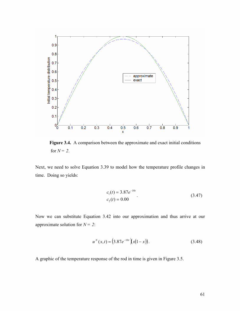
A graphic comparing the approximated and exact initial condition functions is shown in
Figure 3.4.
61
Figure 3.4. A comparison between the approximate and exact initial conditions
for N = 2.
Next, we need to solve Equation 3.39 to model how the temperature profile changes in
time. Doing so yields:
00.0)(87.3)(
2
101
== −
tcetc t
. (3.47)
Now we can substitute Equation 3.42 into our approximation and thus arrive at our
approximate solution for N = 2:
( ) ( )( )xxetxu tN −= − 187.3),( 10 . (3.48)
A graphic of the temperature response of the rod in time is given in Figure 3.5.
62
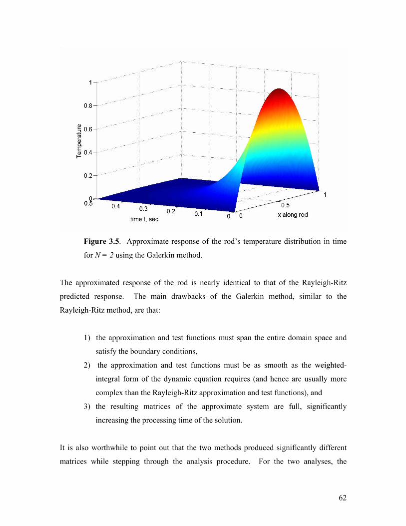
Figure 3.5. Approximate response of the rod’s temperature distribution in time
for N = 2 using the Galerkin method.
The approximated response of the rod is nearly identical to that of the Rayleigh-Ritz
predicted response. The main drawbacks of the Galerkin method, similar to the
Rayleigh-Ritz method, are that:
1) the approximation and test functions must span the entire domain space and
satisfy the boundary conditions,
2) the approximation and test functions must be as smooth as the weighted-
integral form of the dynamic equation requires (and hence are usually more
complex than the Rayleigh-Ritz approximation and test functions), and
3) the resulting matrices of the approximate system are full, significantly
increasing the processing time of the solution.
It is also worthwhile to point out that the two methods produced significantly different
matrices while stepping through the analysis procedure. For the two analyses, the
63
approximation and test functions were purposefully chosen to be different. However, for
this particular example, the test and approximation functions could have been chosen
identically, and in which case, the Rayleigh-Ritz and Galerkin methods would have
produced identical results. For the case of self-adjoint systems like the example heat
equation, where both methodologies are applicable, the Rayleigh-Ritz and Galerkin
methods will be identical.
3.3.3 Comments on Operators and Self-Adjointness
At this juncture it will be worth our while to formally define what is meant by a self-
adjoint system. Firstly, let’s define a linear operator, L (not to be confused with the
variable representing the length of the rod used in the example problems). A linear
operator L is “defined to be an operator if for each )(LDu∈ , there is a uniquely
determined element Lu that lies [in the space defined as] H. Thus, an operator L is linear
if for every complex scalar α and β and for u and v in D(L) the following is true” (Inman,
1989):
LvLuvuL βαβα +=+ )( . (3.49)
The notation D(L) refers to the domain of the linear operator L. An operator is
considered bounded if there exists a finite constant c > 0 such that
ucLu ≤ . (3.50)
In words, Equation 3.50 states that the norm of the operator acting on u must be less than
some finite constant times the norm of u. It can be shown that differential operators are
unbounded operators, whereas integral operators are usually bounded operators.
However, although the differential operators for mechanical systems are unbounded, their
inverses are defined via Green’s functions. Green’s functions are used to determine
integral operators, which are bounded by definition (Inman, 1989). This is important
when defining our next concept, the adjoint of an operator.
64
The adjoint of an operator L is denoted L*. Through the Riesz representation theorem
(see Inman (1989), for instance), the adjoint is defined for all elements )(LDu∈ and
*)(LDv∈ ,
)*,(),( vLuvLu = . (3.51)
The notation of Equation 3.51 defines the inner product, which can formally be expressed
as:
∫Ω
Ω= uvdvu ),( . (3.52)
The Riesz representation theorem requires that the operator, L, be bounded. Further, if L
is bounded, then so, too, is the adjoint L*. Although most mechanical systems of interest
are unbounded, since their inverses are bounded (via Green’s functions) as mentioned
previously, the idea of the adjoint of a differential operator is still used.
An operator is defined to be self-adjoint, even if unbounded, if
*)()( LDLD = (3.53)
and
)(* LDuforuLLu ∈= . (3.54)
Further, if L is self-adjoint, then for all )(, LDvu ∈ ,
),(),( LvuvLu = . (3.55)
65
We now return to our heat conduction problem and wish to discern, for example
purposes, whether or not the operator is self-adjoint. The differential operator is given
by:
2
22
xL
∂∂
−= α , (3.56)
and its domain is defined to be ),0('',',,0)()0(|)( 2rodBrod LLuuuLuuuLD ∈=== . The
notation ),0(2rodB LL means that the function, its first derivative, and its second derivative
are all continuous on the interval ),0( rodL , and is square integrable in the Lebesgue
sense. The subscript B refers to the fact that the function is zero at both ends of the
interval. The Lebesgue integral was developed to satisfy the following property:
∫∫ →
∞→
b
a
b
ann dxxfdxxf )()(lim . (3.57)
Further properties of the Lebesgue integral can be found in the reference (Inman, 1989).
Following Equation 3.55, we have
∫−=rodL
xxvdxuvLu0
2),( α . (3.58)
Integrating Equation 3.58 by parts yields:
∫
∫
−−
++−=−
rod
rod
L
xxx
rodxrodxrodrodx
L
xx
dxuvvu
LvLuvuLvLuvdxu
0
22
222
0
2
)0()0(
)()()0()0()()(
αα
αααα.
(3.59)
66
Equation 3.54 reduces to
∫∫ −+−=−rodrod L
xxxrodrodx
L
xx dxuvvuLvLuvdxu0
222
0
2 )0()0()()( αααα . (3.60)
Since *)(LDv∈ , integration by parts tells us that we need ),0(,, 2rodBxxx LLvandvv ∈ to
ensure that Equation 55 holds true. Therefore, we conclude that
),0(,,,0)()0(|*)( 2rodBxxxrod LLvvvLvvvLD ∈=== . Since D(L) = D(L*) and since we
have demonstrated that Equation 3.50 is true, the heat equation operator is self-adjoint.
3.3.4 The Finite Element Method
As already outlined, the classical variational approximation methods, like Rayleigh-Ritz
and Galerkin, suffer from the difficulty associated with assembling the approximation
and test functions. The fact that the approximation and test functions are arbitrary
(besides having to satisfy certain essential boundary conditions, level of smoothness,
linear independence, completeness, and continuity) is at the heart of the difficulty itself,
and becomes even more complicated if the geometry of the structure becomes
increasingly difficult. The very nature and power of the classical approximation methods
are also their greatest drawback—without a suitable method for choosing quality
approximation functions for the geometry of interest, the level of confidence and quality
of convergence of the resulting approximate solution decreases dramatically.
The power of the finite element method is its ability to divide a complex geometry or
structure into a series of simple domains over which the approximation functions can be
systematically developed. It is in the construction of approximation functions over these
smaller, easier domains that the finite element method significantly differs from the
classical variational methods like Rayleigh-Ritz and Galerkin. This difference, however,
exposes three key features of the finite element method, as summarized from Reddy
(1993):
67
1) Division of the whole into parts, which allows representation of geometrically
complex domains as collections of geometrically simple domains that enable a
systematic derivation of the approximation functions.
2) Derivation of the approximation functions over each element, which often
allows the approximation functions to be algebraic polynomials derived from
interpolation theory.
3) Assembly of elements, which is based on the continuity of the solution and
balance of internal fluxes.
Further, the finite element method is also endowed with the benefit of computational
efficiency due to the symmetrical (in the case of self-adjoint systems), banded-nature of
the developed matrices. Although developed separately from the Rayleigh-Ritz method,
it has been shown that the finite element method is, in fact, a Rayleigh-Ritz method. The
difference between the two, however, is that the classical Rayleigh-Ritz method requires
globally admissible functions where as the finite element method only requires locally
admissible functions (over the smaller, finite element domains). We will now illustrate
the steps of approximating the solution to a differential equation with the finite element
method via the heat conduction example used throughout this chapter.
3.4 Applying the Finite Element Method to the Heat Conduction Problem
As just mentioned, the finite element method is a form of the Rayleigh-Ritz method, and
hence some of the initial procedural work will look similar. However, it will become
quite apparent where the two methods differ, and the advantages of the finite element
method will spring forth.
First, as with the other approximation methods, we start with the strong form of the
dynamics governing the heat conduction within the rod, namely:
Lxfort
txux
txux
≤≤∂
∂=
∂∂
∂∂ 0),(),(2α (3.61)
68
subject to the initial temperature distribution
)()0,( 0 xuxu = (3.62)
and constrained by the following boundary conditions imposed by the ice baths:
0),(),0( == tLutu . (3.63)
As derived previously, we can state the weak form of Equations 3.61-3.63 as follows:
( )( ) 00
2 =+∫L
jtxjx dxuu φφα (3.64)
and where the test functions and approximation functions satisfy:
0)()0( == Ljj φφ . (3.65)
Let’s divide up the rod into four elements of equal length, as shown in Figure 3.6.
69
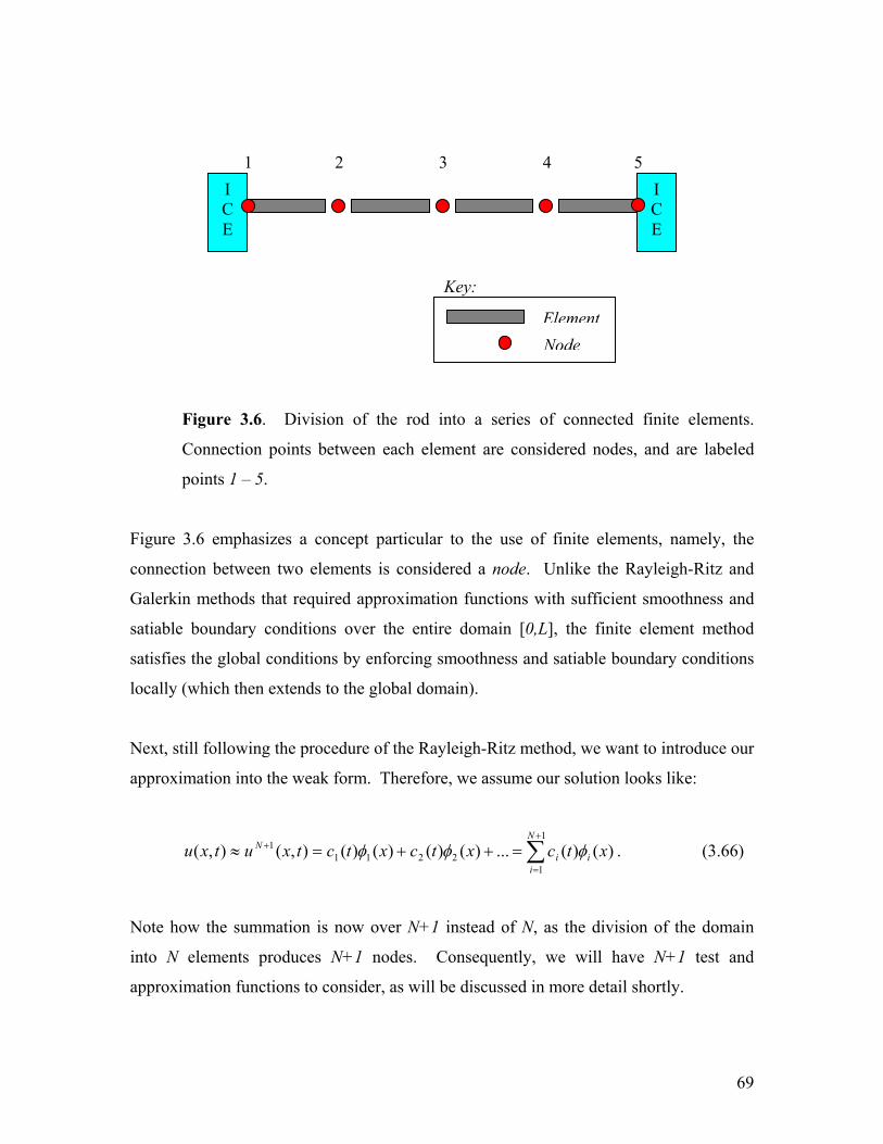
Figure 3.6. Division of the rod into a series of connected finite elements.
Connection points between each element are considered nodes, and are labeled
points 1 – 5.
Figure 3.6 emphasizes a concept particular to the use of finite elements, namely, the
connection between two elements is considered a node. Unlike the Rayleigh-Ritz and
Galerkin methods that required approximation functions with sufficient smoothness and
satiable boundary conditions over the entire domain [0,L], the finite element method
satisfies the global conditions by enforcing smoothness and satiable boundary conditions
locally (which then extends to the global domain).
Next, still following the procedure of the Rayleigh-Ritz method, we want to introduce our
approximation into the weak form. Therefore, we assume our solution looks like:
∑+
=
+ =++=≈1
12211
1 )()(...)()()()(),(),(N
iii
N xtcxtcxtctxutxu φφφ . (3.66)
Note how the summation is now over N+1 instead of N, as the division of the domain
into N elements produces N+1 nodes. Consequently, we will have N+1 test and
approximation functions to consider, as will be discussed in more detail shortly.
5 1
Key:
ICE
ICE
ElementNode
2 3 4
70
Substituting Equation 3.66 into Equation 3.64, we get
( ) ( ) ( )∑ ∫∫∑+
=
+
=
−=1
1 0
2
0
1
1
N
i
L
xjxii
L
ji
N
iti dxcdxc φφαφφ , (3.67)
or, in the matrix notation introduced previously, we have
cKcM v&v 2α−= , (3.68)
where
[ ]
( ) ( )1
1,0
1
1,0
1321
)()(
)()(
)()...()()(
+
=
+
=
+
=
=
=
∫
∫N
ji
L
xjxi
N
ji
L
ji
TN
dxxxK
dxxxM
tctctctcc
φφ
φφ
v
. (3.69)
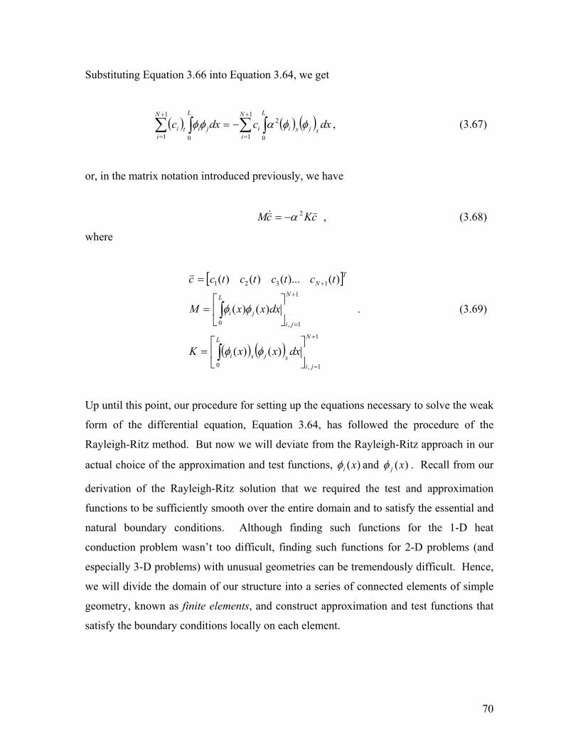
Up until this point, our procedure for setting up the equations necessary to solve the weak
form of the differential equation, Equation 3.64, has followed the procedure of the
Rayleigh-Ritz method. But now we will deviate from the Rayleigh-Ritz approach in our
actual choice of the approximation and test functions, )(xiφ and )(xjφ . Recall from our
derivation of the Rayleigh-Ritz solution that we required the test and approximation
functions to be sufficiently smooth over the entire domain and to satisfy the essential and
natural boundary conditions. Although finding such functions for the 1-D heat
conduction problem wasn’t too difficult, finding such functions for 2-D problems (and
especially 3-D problems) with unusual geometries can be tremendously difficult. Hence,
we will divide the domain of our structure into a series of connected elements of simple
geometry, known as finite elements, and construct approximation and test functions that
satisfy the boundary conditions locally on each element.
71
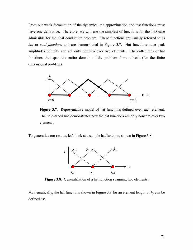
From our weak formulation of the dynamics, the approximation and test functions must
have one derivative. Therefore, we will use the simplest of functions for the 1-D case
admissible for the heat conduction problem. These functions are usually referred to as
hat or roof functions and are demonstrated in Figure 3.7. Hat functions have peak
amplitudes of unity and are only nonzero over two elements. The collections of hat
functions that span the entire domain of the problem form a basis (for the finite
dimensional problem).
Figure 3.7. Representative model of hat functions defined over each element.
The bold-faced line demonstrates how the hat functions are only nonzero over two
elements.
To generalize our results, let’s look at a sample hat function, shown in Figure 3.8.
Figure 3.8. Generalization of a hat function spanning two elements.
Mathematically, the hat functions shown in Figure 3.8 for an element length of he can be
defined as:
x
1 1−iφ iφ
ix1−ix
1+iφ
1+ix
x
1
x=0 x=L
72
≤≤−−
≤≤−−
= ++
+
−−
−
elsewhere
xxxforxxxx
xxxforxxxx
iiii
i
iiii
i
i
0
11
1
11
1
φ (3.70)
However, as in the case of the heat conduction problem as shown in Figure 3.7, the
leftmost and rightmost elements are different from the middle two elements in that their
nodal values at the boundary of the domain [0, L] are known explicitly due to the
presence of the ice baths. These elements that lie on the boundary are known as
boundary elements, and correspondingly, we will require modified approximation and
test functions to take into account the specific boundary conditions pertaining to the
particular problem.
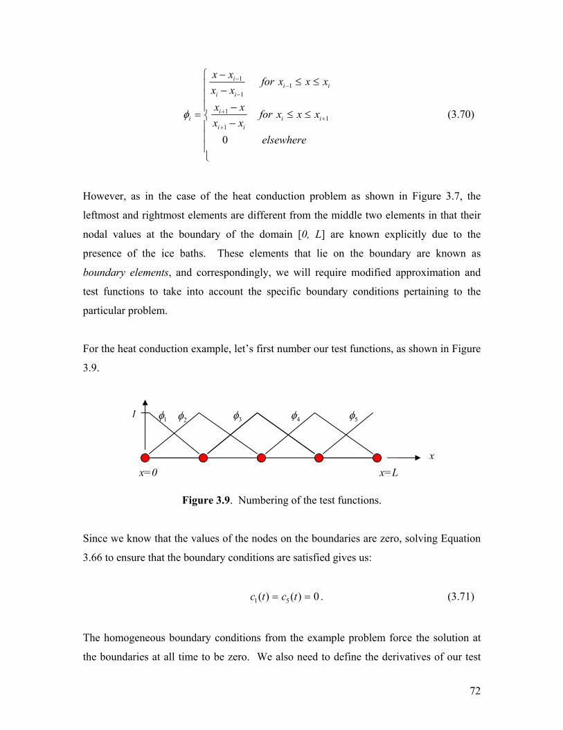
For the heat conduction example, let’s first number our test functions, as shown in Figure
3.9.
Figure 3.9. Numbering of the test functions.
Since we know that the values of the nodes on the boundaries are zero, solving Equation
3.66 to ensure that the boundary conditions are satisfied gives us:
0)()( 51 == tctc . (3.71)
The homogeneous boundary conditions from the example problem force the solution at
the boundaries at all time to be zero. We also need to define the derivatives of our test
x
1
x=0 x=L
1φ 2φ 3φ 4φ 5φ
73
functions, as dictated by the definition of the K matrix in Equation 3.70. The derivative
of each test function is defined by
≤≤−
−
≤≤−
= ++
−−
elsewhere
xxxforxx
xxxforxx
dxd
iiii
iiii
i
0
1
1
11
11
φ . (3.72)
Now that we’ve defined our test functions, we can go ahead and solve our approximate
solution. As before, we will assume that L = 1 cm. Plugging in our test and
approximation functions, as defined by Equations 3.70 and 3.72, we get the following M
and K matrices (from Equations 3.69):
=
121
241000
241
61
24100
0241
61
2410
00241
61
241
000241
121
M (3.73)
−−−
−−−−
−
=
4400048400
048400048400044
K (3.74)
It is important to recognize that a convenient byproduct of the finite element method is
that the resulting matrices (like Equations 3.73 and 3.74) are both banded and symmetric.
Thus, the computational time and efficiency can be readily increased when compared to
74
the classical variational methods. Further, because of the homogeneous boundary
conditions of the problem, the number of unknown coefficients is reduced from 5 to 3.
Such a condition arises because the values of the nodes at the boundaries are known to be
zero. Therefore, the matrices given in Equations 3.73 and 3.74 can be reduced to:
=
61
2410
241
61
241
0241
61
M (3.75)
−−−
−=
840484
048K (3.76)
Next, we need to formulate our initial conditions for the heat conduction problem in the
finite element approximation sense.
As before, we will assume that the initial temperature distribution along the rod is given
by
( )xxu πsin)0,( = . (3.77)
Then, following the construction of the weak form, we have
∫∫==
+ =1
0
1
0
1 )()0,()()0,(L
j
L
jN dxxxudxxxu φφ . (3.78)
Plugging in our approximation, we have:
∫∫∑ =+
=
1
0
1
0
1
1)()0,()()()0( dxxxudxxxc jj
N
iii φφφ . (3.79)
75
Substituting in our shorthand notation from Equation 3.64 and our initial condition we get
( )∫=1
0
)(sin)0( dxxxcM jφπv . (3.80)
Finally, we can solve for the coefficients cv by solving
( )1
1
1
0
1 )(sin)0(+
=
−
= ∫
N
j
j dxxxMc φπv . (3.81)
Solving Equation 3.81 and augmenting the known zero values at the boundaries yields:
=
074.1556.074.10
)0(cv . (3.77)
A comparison between the approximated initial conditions and the exact initial conditions
is shown in Figure 3.10.
76
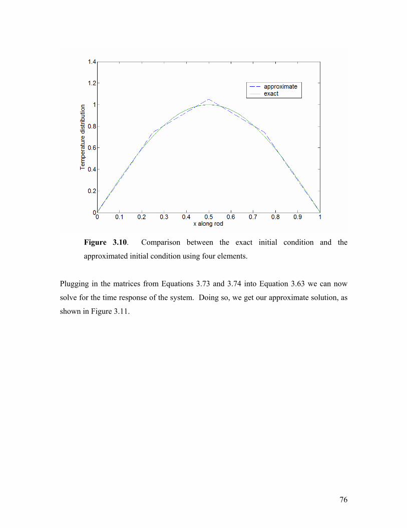
Figure 3.10. Comparison between the exact initial condition and the
approximated initial condition using four elements.
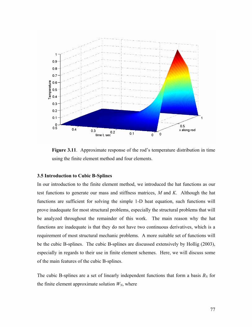
Plugging in the matrices from Equations 3.73 and 3.74 into Equation 3.63 we can now
solve for the time response of the system. Doing so, we get our approximate solution, as
shown in Figure 3.11.
77
Figure 3.11. Approximate response of the rod’s temperature distribution in time
using the finite element method and four elements.
3.5 Introduction to Cubic B-Splines
In our introduction to the finite element method, we introduced the hat functions as our
test functions to generate our mass and stiffness matrices, M and K. Although the hat
functions are sufficient for solving the simple 1-D heat equation, such functions will
prove inadequate for most structural problems, especially the structural problems that will
be analyzed throughout the remainder of this work. The main reason why the hat
functions are inadequate is that they do not have two continuous derivatives, which is a
requirement of most structural mechanic problems. A more suitable set of functions will
be the cubic B-splines. The cubic B-splines are discussed extensively by Hollig (2003),
especially in regards to their use in finite element schemes. Here, we will discuss some
of the main features of the cubic B-splines.
The cubic B-splines are a set of linearly independent functions that form a basis BN for
the finite element approximate solution WN, where
78
,0)0(')0(:)1,()( 3 ==∈= ssStsWN π (3.78)
and where )(3 πS denotes the set of cubic splines with nodes at π (Strang and Fix, 1973).
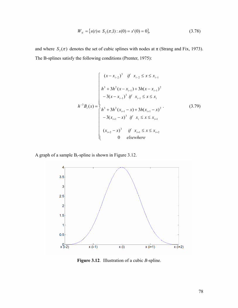
The B-splines satisfy the following conditions (Prenter, 1975):
≤≤−
≤≤−−
−+−+
≤≤−−
−+−+
≤≤−
=
+++
++
++
−−
−−
−−−
−
elsewherexxxifxx
xxxifxx
xxhxxhh
xxxifxx
xxhxxhh
xxxifxx
xBh
iii
iii
ii
iii
ii
iii
i
0)(
)(3
)(3)(3
)(3
)(3)(3
)(
)(
213
2
13
1
211
23
13
1
211
23
123
2
3 . (3.79)
A graph of a sample Bi-spline is shown in Figure 3.12.
Figure 3.12. Illustration of a cubic B-spline.
79
An important feature of the cubic B-splines stems immediately from Figure 3.12. Unlike
the hat functions, notice that the B-splines extend over the range of four elements (or 5
nodes), as opposed to the hat functions that extend over two elements (or 3 nodes).
Hence, the B-splines demonstrate greater connectivity among the elements of the
discretized system. Since they demonstrate greater connectivity, the cubic B-splines do
not require nearly as many elements to obtain sufficiently accurate numerical results
(Hollig, 2003). Another important observation is that unlike more traditional finite
elements, the cubic B-splines have only one degree of freedom per node; but again, the
greater connectivity between elements enables numerical accuracy with fewer elements.
In most structural mechanics problems, typical boundary conditions that must be satisfied
include free, pinned, and clamped ends. The B-splines that overlap boundary elements
can easily be modified to accommodate the necessary boundary conditions. On a free
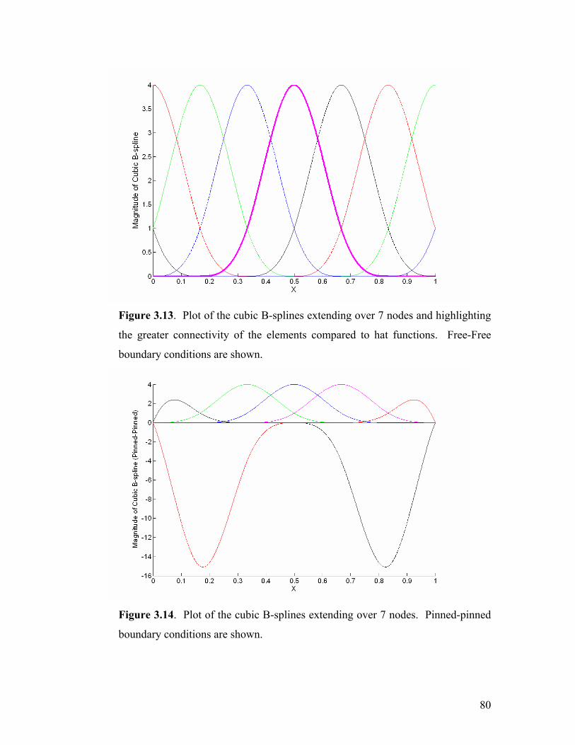
end, no modification is necessary. On a pinned end, the B-splines must be modified such
that the magnitude at the boundary node is zero and the magnitude of the second
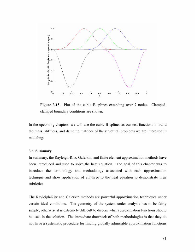
derivative of the boundary node is zero. On a clamped end, the boundary node must have
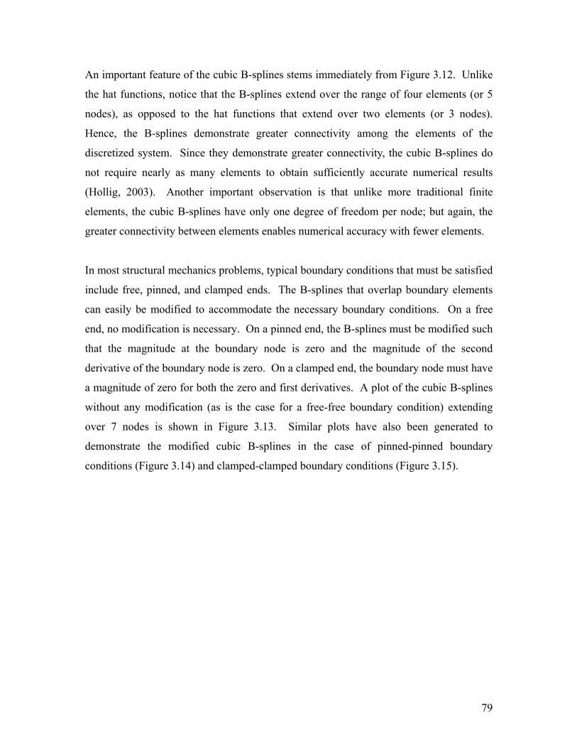
a magnitude of zero for both the zero and first derivatives. A plot of the cubic B-splines
without any modification (as is the case for a free-free boundary condition) extending
over 7 nodes is shown in Figure 3.13. Similar plots have also been generated to
demonstrate the modified cubic B-splines in the case of pinned-pinned boundary
conditions (Figure 3.14) and clamped-clamped boundary conditions (Figure 3.15).
80
Figure 3.13. Plot of the cubic B-splines extending over 7 nodes and highlighting
the greater connectivity of the elements compared to hat functions. Free-Free
boundary conditions are shown.
Figure 3.14. Plot of the cubic B-splines extending over 7 nodes. Pinned-pinned
boundary conditions are shown.
81
Figure 3.15. Plot of the cubic B-splines extending over 7 nodes. Clamped-
clamped boundary conditions are shown.
In the upcoming chapters, we will use the cubic B-splines as our test functions to build
the mass, stiffness, and damping matrices of the structural problems we are interested in
modeling.
3.6 Summary
In summary, the Rayleigh-Ritz, Galerkin, and finite element approximation methods have
been introduced and used to solve the heat equation. The goal of this chapter was to
introduce the terminology and methodology associated with each approximation
technique and show application of all three to the heat equation to demonstrate their
subtleties.
The Rayleigh-Ritz and Galerkin methods are powerful approximation techniques under
certain ideal conditions. The geometry of the system under analysis has to be fairly
simple, otherwise it is extremely difficult to discern what approximation functions should
be used in the solution. The immediate drawback of both methodologies is that they do
not have a systematic procedure for finding globally admissible approximation functions

82
(especially for 2 or 3-D cases). Further, the resulting matrices are fully populated,
making computation of larger system matrices fairly intensive.
The finite element method is a form of the Rayleigh-Ritz method, but has the powerful
benefit of a systematic procedure for finding admissible approximation functions over
each element. Extremely complex geometries can be broken up into finely-meshed
elements of simple geometry, and consequently the assembling of all system matrices is
an easy task through the use of computers. Although the finite element method requires
much greater matrix sizes, the method leads to banded, symmetric matrices that are more
computationally efficient. We also introduced the cubic B-splines, a set of linearly
independent functions that form a basis suitable for the types of structural problems we
are interested in solving.
Now that we have introduced the key concepts behind the Rayleigh-Ritz, Galerkin, and
finite element methods, we will now begin our study of membranes and thin plates with
application to optical and radar-based surface applications.