Chapter 3. Classical Demand Theory

Advanced Microeconomics

Chapter 3. Classical Demand Theory

3.A. Introduction: Take ! as the primitive

(1) What assumption(s) on ! do we need to represent ! with a utility function?

(2) How to perform utility maximization and derive the demand function?

(3) How to derive the utility as a function of prices and wealth, or the indirect utility

function?

(4) How to perform expenditure minimization and derive the expenditure function?

(5) How are demand function, indirect utility function, and expenditure function re-

lated?

3.B. Preference Relations: Basic Properties/Assumptions

In the classical approach to consumer demand, the analysis of consumer behavior begins

by specifying the consumer’s preferences over the commodity bundles in the consumption

set. Consumption set is defined as X ⊂ RL+. Consumer’s preferences are captured by the

preference relation !.

Rationality We would assume Rationality (Completeness and Transitivity) throughout

the chapter. Definition 3.B.1 below repeats the formal definition of Rationality.

Definition 3.B.1. The preference relation ! on X is rational if it possesses the following

two properties:

(i) Completeness: For all x, y ∈ X, we have x ! y or y ! x (or both).

(ii) Transitivity: For all x, y, z ∈ X, if x ! y and y ! z, then x ! z.

Desirability Assumptions The first Desirability Assumption we consider is Monotonic-

ity: larger amounts of commodities are preferred to smaller ones.

1


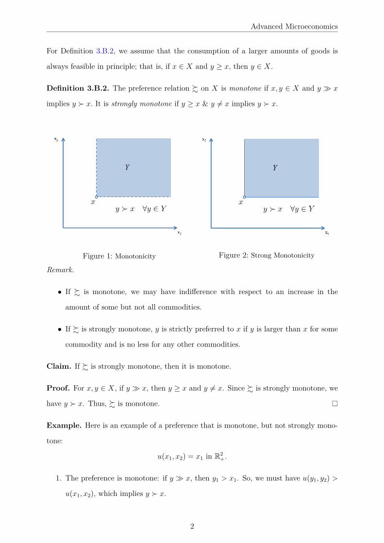
For Definition 3.B.2, we assume that the consumption of a larger amounts of goods is

always feasible in principle; that is, if x ∈ X and y ≥ x, then y ∈ X.

Definition 3.B.2. The preference relation ! on X is monotone if x, y ∈ X and y ≫ x

implies y ≻ x. It is strongly monotone if y ≥ x & y ∕= x implies y ≻ x.

Figure 1: Monotonicity Figure 2: Strong Monotonicity

Remark.

• If ! is monotone, we may have indifference with respect to an increase in the

amount of some but not all commodities.

• If ! is strongly monotone, y is strictly preferred to x if y is larger than x for some

commodity and is no less for any other commodities.

Claim. If ! is strongly monotone, then it is monotone.

Proof. For x, y ∈ X, if y ≫ x, then y ≥ x and y ∕= x. Since ! is strongly monotone, we

have y ≻ x. Thus, ! is monotone.

Example. Here is an example of a preference that is monotone, but not strongly mono-

tone:

u(x1, x2) = x1 in R2+.

1. The preference is monotone: if y ≫ x, then y1 > x1. So, we must have u(y1, y2) >

u(x1, x2), which implies y ≻ x.

2


2. The preference is not strongly monotone: For x = (1, 2) and y = (1, 3), we have

y ≥ x, but u(y) = u(x), which implies y ∼ x.

For much of the theory, a weaker desirability assumption, local nonsatiation, suffices.

Definition 3.B.3. The preference relation ! on X is locally nonsatiated if for every

x ∈ X and every ε > 0, ∃y ∈ X such that ‖y − x‖ ≤ ε and y ≻ x.

Figure 3: Test for Local Nonsatiation

Claim. Local nonsatiation is a weaker desirability assumption compared to monotonicity.

If ! is monotone, then it is locally nonsatiated.

Proof. Fix some ε > 0, Let there be an arbitrary x ∈ X and e = (1, · · · , 1). For any

λ > 0, we also have y = x + λe ∈ X. Since clearly y = x + λe ≫ x, by monotonicity,

y ≻ x. On the other hand, ‖y − x‖ =√

Lλ2 = λ√

L. Thus, for λ < ε√L

, ‖y − x‖ ≤ ε.

Since x is arbitrary, the existence of the point y = x + λe where λ < ε√L

implies that !

is locally nonsatiated.

Example. Here is an example of a preference that is locally nonsatiated, but not mono-

tone:

u(x1, x2) = x1 − |1 − x2| in R2+.

1. The preference is locally nonsatiated: Fix an ε > 0. We can find λ > 0 such that

λ < ε. Denote y = (y1, y2) = (x1 + λ, x2). Then u(y) − u(x) = λ > 0, which

3


implies y ≻ x. On the other hand, ‖y − x‖ =√

λ2 = λ < ε. Therefore, ! is locally

nonsatiated.

2. The preference is not monotone: For x = (1, 1) and y = (1.5, 2), we have y ≫ x,

but u(x) = 1 > u(y) = 0.5, which implies x ≻ y.

Indifference sets Given ! and x, we can define 3 related sets of consumption bundles.

1. The indifferent set is {y ∈ X : y ∼ x}.

2. The upper contour set is {y ∈ X : y ! x}.

3. The lower contour set is {y ∈ X : x ! y}.

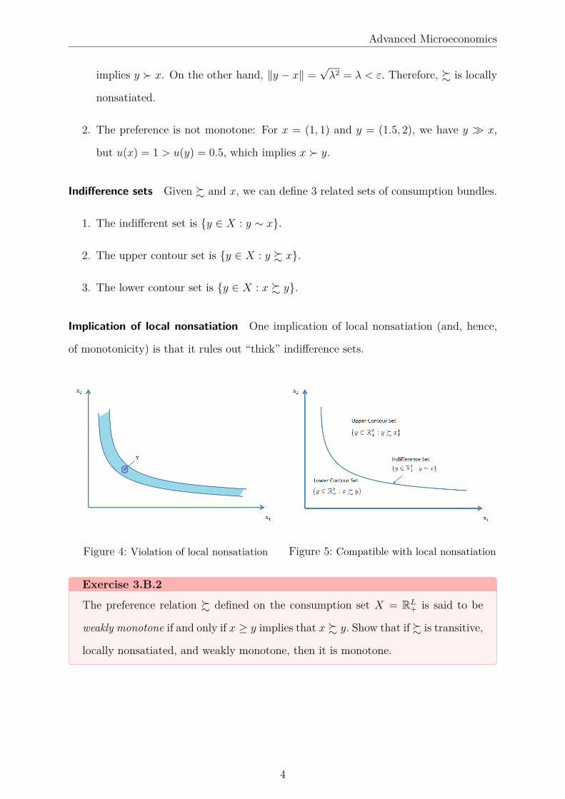
Implication of local nonsatiation One implication of local nonsatiation (and, hence,

of monotonicity) is that it rules out “thick” indifference sets.

Figure 4: Violation of local nonsatiation Figure 5: Compatible with local nonsatiation

Exercise 3.B.2

The preference relation ! defined on the consumption set X = RL+ is said to be

weakly monotone if and only if x ≥ y implies that x ! y. Show that if ! is transitive,

locally nonsatiated, and weakly monotone, then it is monotone.

4


Convexity Assumptions

Definition 3.B.4. The preference relation ! on X is convex if for every x ∈ X, the

upper contour set of x, {y ∈ X : y ! x} is convex; that is, if y ! x and z ! x, then

αy + (1 − α)z ! x for any α ∈ [0, 1].

Figure 6: Convex Preference Figure 7: Nonconvex Preference

Properties associated with convexity

(i) Diminishing marginal rates of substitution: with convex preferences, from any ini-

tial consumption X, and for any two commodities, it takes an increasingly larger

amounts of one commodity to compensate for successive unit losses of the other.

(ii) Preference for diversity (implied by (i)): under convexity, if x is indifferent to y,

then 12x + 1

2y cannot be worse than x or y.

Definition 3.B.5. The preference relation ! on X is strictly convex if for every x ∈ X,

we have that y ! x and z ! x, and y ∕= z implies αy + (1 − α)z ≻ x for all α ∈ (0, 1).

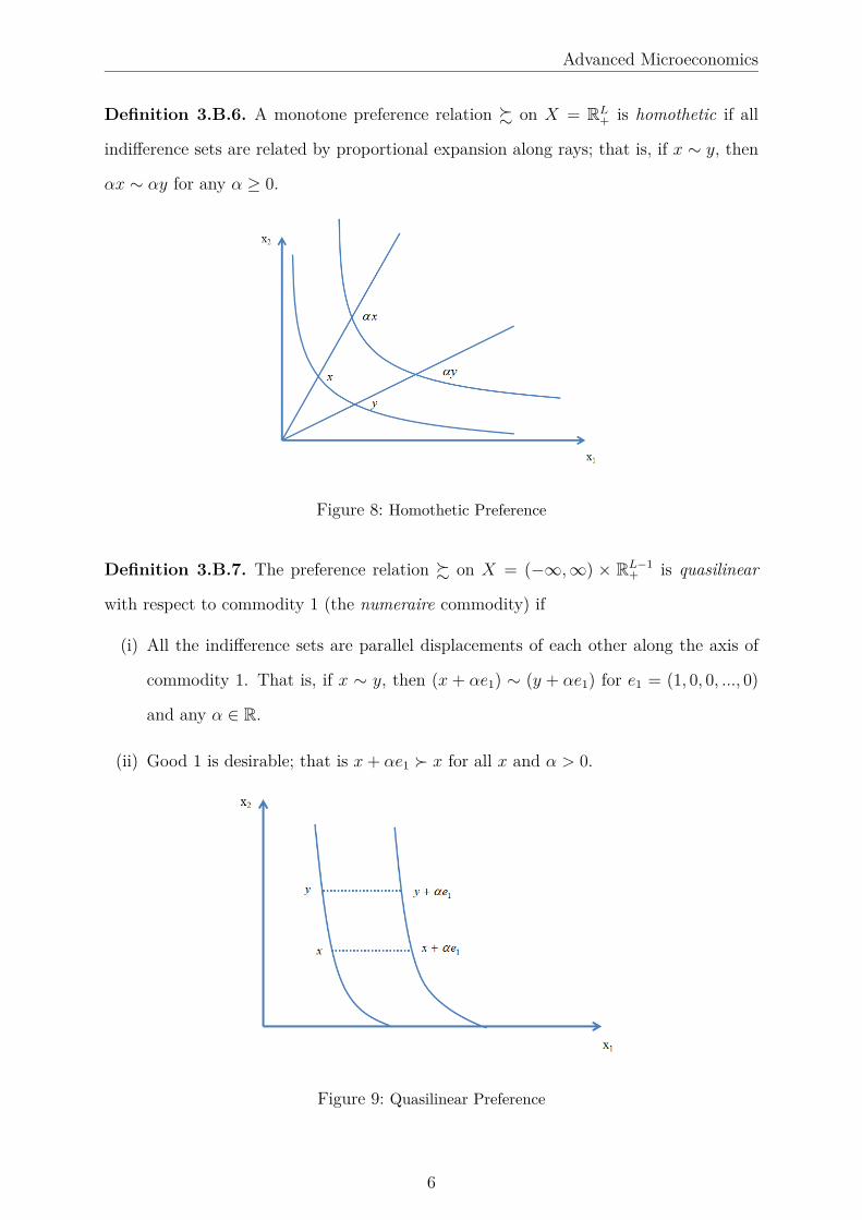
Homothetic and Quasilinear Preference In applications (particularly those of an

econometric nature), it is common to focus on preferences for which it is possible to

deduce the consumer’s entire preference relation from a single indifference set. Two ex-

amples are the classes of homothetic and quasilinear preferences.

5


Definition 3.B.6. A monotone preference relation ! on X = RL+ is homothetic if all

indifference sets are related by proportional expansion along rays; that is, if x ∼ y, then

αx ∼ αy for any α ≥ 0.

Figure 8: Homothetic Preference

Definition 3.B.7. The preference relation ! on X = (−∞, ∞) × RL−1+ is quasilinear

with respect to commodity 1 (the numeraire commodity) if

(i) All the indifference sets are parallel displacements of each other along the axis of

commodity 1. That is, if x ∼ y, then (x + αe1) ∼ (y + αe1) for e1 = (1, 0, 0, ..., 0)

and any α ∈ R.

(ii) Good 1 is desirable; that is x + αe1 ≻ x for all x and α > 0.

Figure 9: Quasilinear Preference

6


3.C. Preference and Utility

Key Question. When can a rational preference relation be represented by a utility

function?

Answer: If the preference relation is continuous.

Definition 3.C.1. The preference relation ! on X is continuous if it is preserved in the

limits. That is, for any sequence of pairs {(xn, yn)}∞n=1 with xn ! yn for all n, x = lim

n→∞xn,

y = limn→∞

yn, we have x ! y.

Interpretation: Consumer’s preferences cannot exhibit jumps. The consumer cannot

prefer each elements in the sequence xn to the corresponding element in the sequence yn

but suddenly reverse her preference at the limiting points of these sequences x and y.

Claim 1. ! is continuous if and only if for all x, the upper contour set {y ∈ X : y ! x}

and the lower contour set {y ∈ X : x ! y} are both closed.

Proof. We only provide the proof for “only if” part. “if” part is more advanced and not

required by this course.

Definition 3.C.1 implies that for any sequence of points {yn}∞n=1 with x ! yn for all n

and y = limn→∞

yn, we have x ! y (just let xn = x for all n). Hence the closedness of lower

contour set is implied. Similarly, we could show the closedness of upper contour set.

In fact, we have a similar statement about continuous functions. We leave its proof as

an exercise.

Exercise

Claim 2. A function f : RL → R is continuous if and only if for all a, the set

{x ∈ RL : f(x) ≥ a} and the set {x ∈ RL : f(x) ≤ a} are both closed.

Prove the “only if” part of the claim above.

We would use the Claims 1 & 2 to prove the famous Debreu’s theorem later.

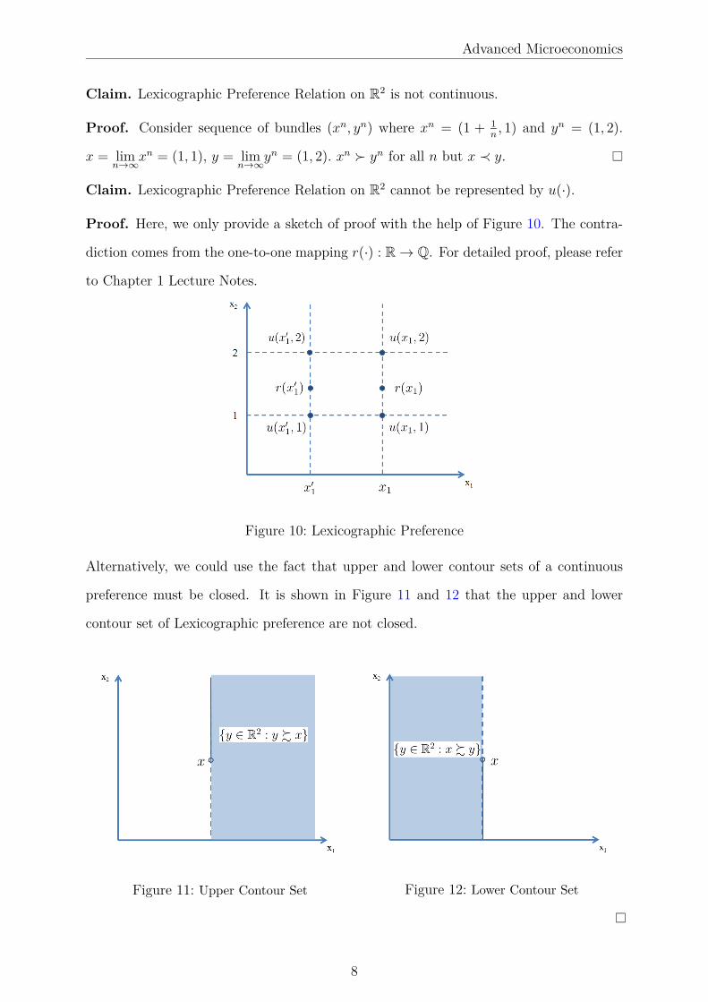
Example 3.C.1. Lexicographic Preference Relation on R2

x ≻ y if either x1 > y1, or x1 = y1 and x2 > y2.

x ∼ y if x1 = y1 and x2 = y2.

7


Claim. Lexicographic Preference Relation on R2 is not continuous.

Proof. Consider sequence of bundles (xn, yn) where xn = (1 + 1n, 1) and yn = (1, 2).

x = limn→∞

xn = (1, 1), y = limn→∞

yn = (1, 2). xn ≻ yn for all n but x ≺ y.

Claim. Lexicographic Preference Relation on R2 cannot be represented by u(·).

Proof. Here, we only provide a sketch of proof with the help of Figure 10. The contra-

diction comes from the one-to-one mapping r(·) : R → Q. For detailed proof, please refer

to Chapter 1 Lecture Notes.

Figure 10: Lexicographic Preference

Alternatively, we could use the fact that upper and lower contour sets of a continuous

preference must be closed. It is shown in Figure 11 and 12 that the upper and lower

contour set of Lexicographic preference are not closed.

Figure 11: Upper Contour Set Figure 12: Lower Contour Set

8


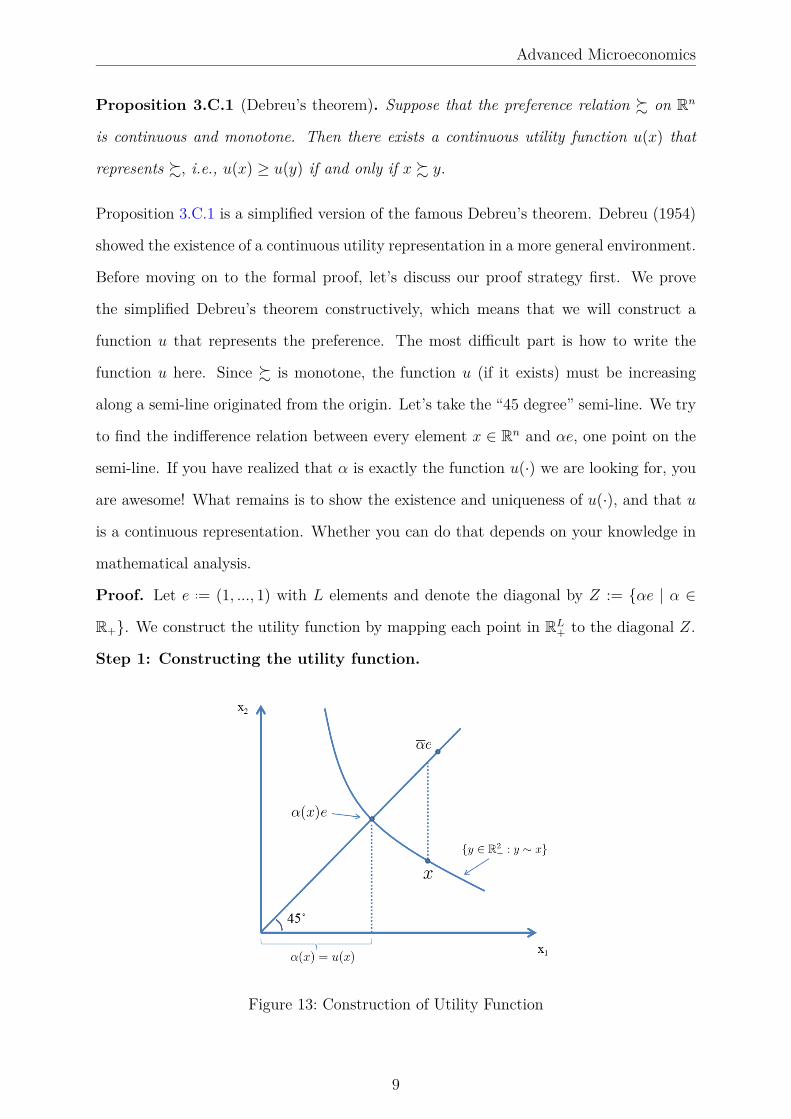
Proposition 3.C.1 (Debreu’s theorem). Suppose that the preference relation ! on Rn

is continuous and monotone. Then there exists a continuous utility function u(x) that

represents !, i.e., u(x) ≥ u(y) if and only if x ! y.

Proposition 3.C.1 is a simplified version of the famous Debreu’s theorem. Debreu (1954)

showed the existence of a continuous utility representation in a more general environment.

Before moving on to the formal proof, let’s discuss our proof strategy first. We prove

the simplified Debreu’s theorem constructively, which means that we will construct a

function u that represents the preference. The most difficult part is how to write the

function u here. Since ! is monotone, the function u (if it exists) must be increasing

along a semi-line originated from the origin. Let’s take the “45 degree” semi-line. We try

to find the indifference relation between every element x ∈ Rn and αe, one point on the

semi-line. If you have realized that α is exactly the function u(·) we are looking for, you

are awesome! What remains is to show the existence and uniqueness of u(·), and that u

is a continuous representation. Whether you can do that depends on your knowledge in

mathematical analysis.

Proof. Let e ..= (1, ..., 1) with L elements and denote the diagonal by Z := {αe | α ∈

R+}. We construct the utility function by mapping each point in RL+ to the diagonal Z.

Step 1: Constructing the utility function.

Figure 13: Construction of Utility Function

9


• Denote by A+ := {α ∈ R+ : αe ! x} the diagonal points that are weakly better

than x, and A− := {α ∈ R+ : x ! αe} the diagonal points that are weakly worse

than x.

• Continuity of preference implies that A+ is closed. Note that A+ is bounded from

below by 0, and thus we obtain A+ = [αL, ∞) for some αL ≥ 0.

• Similarly, A− = [0, αU ] for some αU ≥ 0.

• Since αLe ! x ! αUe, by monotonicity αL ≥ αU .

• We must also have αL = αU . Otherwise, there exists some real number α′ ∈ (αU , αL)

such that both α′ ! x and α′ ≾ x fail.

• Therefore, we map each x ∈ RL+ to some point αLe (or αUe) on the diagonal. Define

u(x) := αL and we have x ∼ u(x)e.

Step 2: Proving that u(x) represents !.

• It suffices to show that u(x) ≥ u(y) iff x ! y.

• Since x ∼ u(x)e,

u(x) ≥ u(y) ⇐⇒ u(x)e ! u(y)e ⇐⇒ x ! y.

The first “iff” part holds by monotonicity. The second “iff” part holds by our

definition of u(x).

Step 3: Proving that u(x) is continuous.

• Since ! is a continuous preference, the upper contour set {x ∈ Rn : x ! x′} and

the lower contour set {x ∈ Rn : x′ ! x} are both closed (by Claim 1).

• We have shown that u is indeed a utility representation, and hence {x ∈ Rn : u(x) ≥

u(x′)} and {x ∈ Rn : u(x) ≤ u(x′)} are both closed.

• The construction of the function u ensures that u(x′) can take any value in (0, +∞).

• Therefore, sets {x ∈ Rn : u(x) ≥ a} and {x ∈ Rn : u(x) ≤ a} are both closed. By

Claim 2, u(x) is continuous.

10


Assumptions of differentiability of u(x) The assumption of differentiability is com-

monly adopted for technical convenience, but is not applicable to all useful models.

Here is an example of preference that is not differentiable.

Example (Leontief Preference). x′′ ! x′ if and only if min{x′′1, x′′

2} ≥ min{x′1, x′

2}.

Figure 14: Leontief Preference

u(x1, x2) = min{x1, x2} represents Leontief preference. u(x1, x2) is not differentiable

because of the kink in the indifference curves when x1 = x2, i.e., when x = (x1, x1).

To see this, for the first variable x1 (similar argument applies to the second variable):

limε→0−

u(x1 + ε, x1) − u(x1, x1)ε

= limε→0−

min{x1 + ε, x1} − min{x1, x1}ε

= limε→0−

x1 + ε − x1

ε= 1;

limε→0+

u(x1 + ε, x1) − u(x1, x1)ε

= limε→0+

min{x1 + ε, x1}) − min{x1, x1}ε

= limε→0+

x1 − x1

ε= 0.

Implications of ! and u

(i) ! is convex ⇐⇒ u : X → R is quasi-concave.

(ii) continuous ! on RL+ is homothetic ⇐⇒ it admits an H.D.1 utility function u(x)

(iii) continuous ! on (−∞, ∞) × RL−1+ is quasilinear with respect to Good 1 ⇐⇒ it

admits a utility function of the form u(x) = x1 + φ(x2, ..., xL)1

1In (i), all utility functions representing ! are quasiconcave; whereas (ii) and (iii) merely say thatthere exists at least one utility function that has the specific form.

11


Definition. The utility function u(·) is quasiconcave if the set {y ∈ RL+ : u(y) ≥ u(x)}

is convex for all x or, equivalently, if u(αx + (1 − α)y) ≥ min{u(x), u(y)} for all x, y and

all α ∈ [0, 1]. If u(αx + (1 − α)y) > min{u(x), u(y)} for x ∕= y and α ∈ (0, 1), then u(·)

is strictly quasiconcave.

Proof.

(i) ! is convex. ⇐⇒ If y ! x, z ! x, then αy + (1 − α)z ! x ∀α ∈ [0, 1].

⇐⇒ If u(y) ≥ u(x), u(z) ≥ u(x), then u(αy + (1 − α)z) ≥ u(x) ∀α ∈ [0, 1].

⇐⇒ {y ∈ RL+ : u(y) ≥ u(x)} is convex.

⇐⇒ u : X → R is quasi-concave.

(ii) (a) “⇐”: Suppose u(x) is H.D.1., i.e., u(αx) = αu(x) and u(αy) = αu(y).

Also suppose x ∼ y ⇐⇒ u(x) = u(y).

Then u(αy) = αu(y) = αu(x) = u(αx) =⇒ αx ∼ αy =⇒ ! is homothetic.

(b) “⇒”: We will prove that the utility function constructed in the proof of Propo-

sition 3.C.1, i.e., u(x) defined by u(x)e ∼ x, is H.D.1.

Homothetic ! implies αu(x)e ∼ αx. By definition of u(x), u(αx)e ∼ αx.

Then αu(x)e ∼ u(αx)e =⇒ u(αx) = αu(x) =⇒ u(x) is H.D.1.

(iii) a) “⇐”: Suppose u(x) = x1 + φ(x2, ..., xL). Then, u (x + αe1) = x1 + α +

φ (x2, · · · , xL) = α + u(x). Similarly, u (y + αe1) = α + u(y).

Therefore, x ∼ y =⇒ u(x) = u(y) =⇒ u (x + αe1) = u (y + αe1) =⇒

(x + αe1) ∼ (y + αe1) =⇒ ! is quasilinear.

b) “⇒”: In general, for some consumption bundle (0, x2, · · · , xL), there exists a

consumption bundle (x∗1, 0, · · · , 0), such that (0, x2, · · · , xL) ∼ (x∗

1, 0, · · · , 0).

We therefore define the mapping from (x2, · · · , xL) to x∗1 by a function x∗

1 =

φ (x2, · · · , xL). From ! being quasilinear, we have

(x1, x2, · · · , xL) ∼ (x1 + φ (x2, · · · , xL) , 0, · · · , 0) .

Therefore, ! admits a utility function of the form u(x) = x1+φ(x2, ..., xL).

12


Exercise 3.C.6Suppose that in a two-commodity world, the consumer’s utility function takes the

form u (x) = [α1xρ1 + α2x

ρ2]1/ρ . This utility function is known as the constant elas-

ticity of substitution (or CES) utility function.

(a) Show that when ρ = 1, indifference curves become linear.

(b) Show that as ρ → 0, this utility function comes to represent the same prefer-

ences as the (generalized) Cobb-Douglas utility funciton u (x) = xα11 xα2

2 .

(c) Show that as ρ → −∞, indifference curves become “right angles”; that is, this

utility funciton has in the limit the indifference map of the Leontief utility

function u (x1, x2) = min {x1, x2} .

3.D. Utility Maximization Problem (UMP)

We assume throughout that preference is rational, continuous, and locally nonsatiated,

and we take u(x) to be a continuous utility function representing these preferences. We

also assume that the consumption set is X = RL+.

The consumer’s problem of choosing her most preferred consumption bundle x(p, w) can

be stated as a Utility Maximization Problem (UMP):

maxx∈RL

+

u(x)

s.t. p · x ≤ w

Proposition 3.D.1. If p ≫ 0 and u(·) is continuous, then the utility maximization

problem has a solution.

Proof. Bp,w = {x ∈ RL+ : p · x ≤ w} is compact, i.e,

(i) bounded: 0 ≤ xl ≤ w/pl, for pl > 0

(ii) closed (it contains all the limit points): Proof by contradiction. Consider a sequence

{xn}∞n=1 where xn ∈ Bp,w, or p ·xn ≤ w for all n and x = lim

n→∞xn ∕∈ Bp,w or p ·x > w.

13


There exists ε > 0 such that for all y satisfying ‖y − x‖ < ε, p · y > w. Therefore,

∃N > 0, s.t. ∀n ≥ N, p · xn > w. This contradicts p · xn ≤ w for all n.

By Extreme Value Theorem, a continuous function always has a maximum value on any

compact set.

Here, we provide two counter examples where the solution of UMP does not exists.

Counter Examples.

(i) Bp,w is not closed: p · x < w

(ii) u(x) is not continuous: u(x) =

!"""#

"""$

p · x for p · x < w

0 for p · x = w

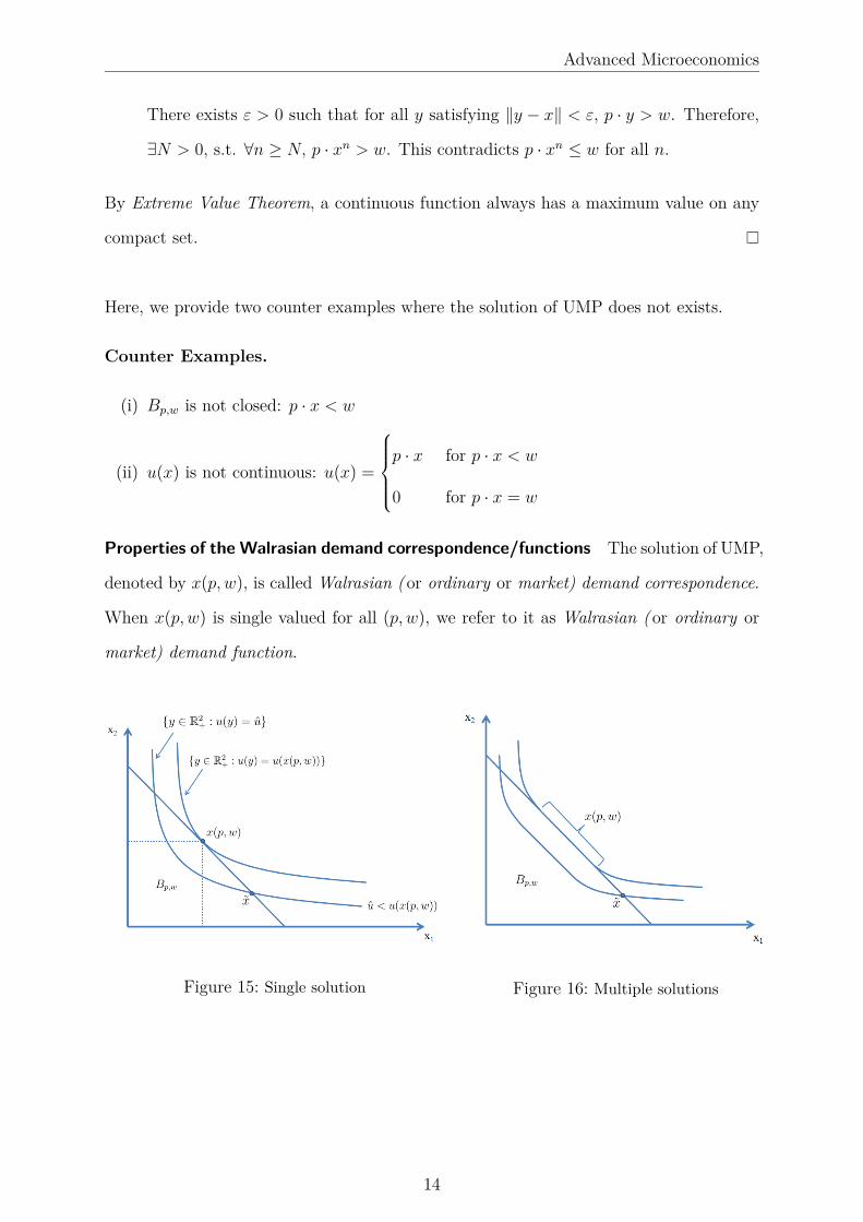
Properties of the Walrasian demand correspondence/functions The solution of UMP,

denoted by x(p, w), is called Walrasian (or ordinary or market) demand correspondence.

When x(p, w) is single valued for all (p, w), we refer to it as Walrasian (or ordinary or

market) demand function.

Figure 15: Single solution Figure 16: Multiple solutions

14


Proposition 3.D.2. Suppose that u(x) is a continuous utility function representing a

locally nonsatiated preference relation ! defined on the consumption set X = RL+. Then

the Walrasian demand correspondence x(p, w) possesses the following properties:

(i) Homogeneity of degree zero in (p, w) : x(αp, αw) = x(p, w) for any p, w and scalar

α > 0.

(ii) Walras’ Law: p · x = w for all x ∈ x(p, w).

(iii) Convexity/uniqueness: If ! is convex, so that u(·) is quasiconcave, then x(p, w) is

a convex set. Moreover, if ! is strictly convex, so that u(·) is strictly quasiconcave,

then x(p, w) consists of a single element.

Recall,

Definition. The preference relation ! on X is convex if for every x ∈ X, the upper

contour set of x, {y ∈ X : y ! x} is convex; that is, if y ! x and z ! x, then

αy + (1 − α)z ! x for any α ∈ [0, 1].

Definition. The utility function u(·) is quasiconcave if the set {y ∈ RL+ : u(y) ≥ u(x)}

is convex for all x or, equivalently, if u(αx + (1 − α)y) ≥ min{u(x), u(y)} for all x, y and

all α ∈ [0, 1].

Proof.

(i) H.D.∅ : {x ∈ RL+ : p · x ≤ w} = {x ∈ RL

+ : αp · x ≤ αw}.

The set of feasible consumption bundles in the UMP is unaffected by α. Therefore,

x(p, w) = x(αp, αw).

(ii) Walras’ Law: Suppose p · x(p, w) < w. Then ∃ε > 0 such that ∀y such that ‖y −

x(p, w)‖ < ε, p · y < w. Local nonsantiation implies ∃y with y ∈ X and ‖y −

x(p, w)‖ < ε such that y ≻ x(p, w) =⇒ contradiction with x(p, w) being optimal.

(iii) Suppose x, x′ ∈ x(p, w) and x ∕= x′. Then u(x) = u(x′). Quasiconcavity of u implies

u(αx + (1 − α)x′) ≥ min{u(x), u(x′)} =⇒ αx + (1 − α)x′ ∈ x(p, w)

15


Now suppose u(x) is strictly quasiconcave. Suppose x, x′ ∈ x(p, w) and x ∕= x′.

Then u(x) = u(x′). Strict quasiconcavity implies u(αx + (1 − α)x′) > u(x) = u(x′).

This contradicts that x, x′ ∈ x(p, w). Therefore, x(p, w) is single valued.

Alternative proof for (iii): Suppose x, x′ ∈ x(p, w). Then x ∼ x′ ! y, ∀y ∈ Bp,w.

x = αx + (1 − α)x′ ! x ∼ x′ =⇒ x ! y, ∀y ∈ Bp,w. Strict convexity x ≻ x ∼ x′

which contradicts x, x′ ∈ x(p, w).

We will take a break to review some mathematical results before proceeding

with this Chapter. Read “Math Review: Maximization Problem” for details.

16

Documents

Chapter 3. Classical Demand Theory