Embed Size (px)
Citation preview
76
CHAPTER 3
ANALYSIS OF RAIL GUN KEY PARAMETERS USING
FINITE ELEMENT ANALYSIS TECHNIQUE
3.1 INTRODUCTION
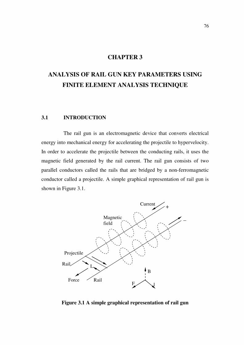
The rail gun is an electromagnetic device that converts electrical
energy into mechanical energy for accelerating the projectile to hypervelocity.
In order to accelerate the projectile between the conducting rails, it uses the
magnetic field generated by the rail current. The rail gun consists of two
parallel conductors called the rails that are bridged by a non-ferromagnetic
conductor called a projectile. A simple graphical representation of rail gun is
shown in Figure 3.1.
Current
Magnetic
field
Projectile
Rail
RailForce
+
_
B
F l
L
Figure 3.1 A simple graphical representation of rail gun
77
The current flows through one rail, passes through the projectile
normal to the rails, and then passes through other rail in parallel. As a result,
the two rails produce the magnetic field and an intercepting field is produced
by the armature. The current flowing through armature interacts with the
magnetic field created by the rail current and produces an accelerating force
on an armature called Lorentz force.
In order to design a 500-kJ pulsed power supply, using computer
simulation techniques, to obtain the desired velocity of the rail gun,
inductance gradient of the rails is needed. The inductance gradient value
mainly depends on rail dimensions and designs. In order to get higher value of
projectile velocity proper rail dimensions and designs have to be selected.
Choosing the rail dimensions and rail designs are dependent on rail gun key
parameters such as inductance gradient of the rails, magnetic flux density
between the rails, current distribution in rails, repulsive force acting on the
rails, and temperature distribution in rails. The magnetic flux density between
the rails and inductance gradient of the rails plays an important role in the rail
gun which determines directly the force that accelerates the projectile. The
repulsive force acting on the rails is not exactly calculated as short
acceleration pulse current produces non linear effect and uneven current
distribution. The rail gun is supplied with large current which rise very
quickly and drives the armature down the rails. As a result, thermal energy is
generated which changes the electrical and thermal properties of the rail
materials. Hence, in order to gain a quantitative understanding of these
parameters, it is desirable to calculate them well in advance. In general, these
values are affected by number of parameters such as velocity of the moving
armature, armature and rail geometry, rail dimensions, armature and rail
materials (Bok-ki kim et al 1999). Asghar Keshtkar (2005) has calculated the
inductance gradient value of rails with respect to rail dimensions using
transient analysis finite element method. Jerry Kerrisk (1984) has calculated
78
the inductance gradient values, current density distribution in the rails, and
temperature distribution in the rails with respect to the rail dimensions. He has
used, A.C in the high frequency limit, finite difference method to carry out
this investigation. Honjo et al (1986) have calculated the force acting on rail
conductors using BUS 3-D program. Azzerboni et al (1993) have developed
numerical code, called FEMM, to calculate the force acting on the rails.
Huerta et al (1991) have calculated the inductance gradient of the rails using
conformal mapping method. Ellies et al (1995) have studied the influence of
bore and rail geometry by using 2-D, A.C finite element method with high
frequency limit. Patch et al (1984) have analyzed the rail barrel design using
A.C analysis. From the above literature review, it is observed that for the past
several years, various numerical and analytical methods were developed to
compute the rail gun key parameters. These parameters can be calculated
either by transient analysis or A.C method in the high frequency limit. In this
case, all the current is distributed on the surface of the conductor. This is a
good approximation for rail guns with good conductor (Asghar Keshtkar
2005). In this work, finite element analysis software package, named Maxwell
Electro Magnetic Field Solver, is employed to calculate the rail gun
parameters using 2-D, A.C method in the high frequency limit. The study is
made to explore a range of bore and rail geometry and look at their effect on
key rail gun system parameters.
3.2 KEY ACCELERATOR PARAMETERS
Important accelerator design parameters of rail gun includes
1. Inductance gradient of the rails
2. Current density distribution over a rail cross sections
3. Magnetic flux density distribution between the rails
4. Rail separation force acting on the rails
5. Temperature distribution in the rails
79
3.2.1 Inductance Gradient of the Rails
Inductance gradient of the rails plays an important role in the rail
gun design as it determines the efficiency of the rail gun. Efficiency of the rail
gun is defined as the ratio of projectile energy to input energy. To improve the
efficiency of the rail gun, various geometry and dimensions of rails and
armature are used. The Acceleration force and L’ could be investigated
instead of efficiency (Asghar Keshtkar 2005). These are related by the
following equation
' 21
2F LI (3.1)
where L’ is the gradient inductance or inductance per unit length of the
rails in µH/m
I is the driving current in Amps and
F ’ is the force exerted on the armature in Newton
3.2.2 Current Density Distribution in a Rail
One of the biggest problems in the analysis of rail gun is the
determination of the current density distribution in the massive moving
conducting parts. The knowledge of the current density distribution over a rail
cross section against time is very important for prediction of the behavior of
the system. The current concentration determines the joule energy that
dissipated in the rails, their temperature rise, electromagnetic stress on the
rails, and it provides useful information about correct utilization of the
materials. Moreover, the accelerating time, the escape velocity and the
accelerating pressure are influenced by the current density in the rails
(Azzerboni et al 1992). As a very high value of current and short duration
pulse is applied to the rail gun the current distribution is not uniform over the
80
cross section. In this case, current is distributed in a very thin layer near the
surface of each conductor that is called skin depth. Moreover, the current
density is higher at the rails inner edges. This phenomenon produces a hot
spot that fuses the rail edges (Asghar Keshtkar 2005). In order to prevent rails
damage due to ohmic heating and internal forces, it is necessary to understand
the current density distribution within the conducting medium.
3.2.3 Rail Separation Force Acting on the Rails
Any pair of current carrying conductor experiences an attractive
force or repulsive force depending on whether the current is flowing in the
same or opposite direction. The same force which accelerates the projectile
also works to separate the rail pair. In order to mechanically brace the rails
against the high forces which results from the large current, the repulsive
force acting on the rail should be calculated (Honjo et al 1986). The
separation force is not easily calculated. The high current and short
accelerator pulses generate non linear effect and uneven current distribution in
the rails. So the determination of rail separation force is difficult.
3.2.4 Magnetic Flux Density between the Rails (B)
The magnetic field between the rails plays an important role in the
rail gun design as it produces force on the projectile (Micheal Huebschman et
al 1993). The current through the armature interacts with the field produced
by the rail current and produces a force called Lorentz force and given as
(Mohmmad Soleimani et al 2000).
F J Bdv (3.2)
where J is the current density on the armature
B is the magnetic flux density.
81
Force acting on the armature can be computed accurately with the
accurate knowledge of B . Hence, it is necessary to calculate the magnetic
flux density between the rails. The magnetic flux density between the rails is
the summation of the field due to the rails and armature. But the field
contribution between the rails due to armature is negligible when compared
with the field contribution due to the rails, as the length of the armature is less
when compared to the length of the rails. Hence, the magnetic field due to the
rail alone is taken into account for the total magnetic field calculation.
3.2.5 Temperature Distribution in a Rail
Electromagnetic launchers are usually supplied with large current
which rises very quickly and drives the projectile down the rails. The firing
lasts but a few milliseconds at the most because the time is short the current
does not penetrate the rails and the projectile, but rather resides thin layer near
the surface of the conductor. These regions may be heated up by the current
nearly to the melting point of the metal and causes damage to rails. Due to
increase in temperature, the mechanical yield strength of rail gun material is
lowered. The increase in temperature changes the electrical and thermal
specification of constituent parts and makes the structure an inhomogeneous
media (Mohmmad Soleimani et al 2000). In order to prevent rail gun damage
due to ohmic heating, it is necessary to understand temperature distribution
phenomenon within the conducting medium (Long et al 1986).
3.3 PROBLEM STATEMENT
The rail gun key parameters such as the inductance gradient of the
rails, magnetic flux density between the rails, current density over a rail cross
section, repulsive force acting on the rails, and temperature distribution in the
rails are affected by a number of parameter such as velocity of the moving
armature, armature and rail geometry, rail dimensions, armature and rail
82
materials. In the operation of an EML, a few highly coupled phenomena are
present. Hence, the calculations of rail gun key parameters are difficult. In
order to make the calculation tractable, a number of simplifying assumptions
are made. First, the rail gun is a 3-D device, but assuming that its barrel is
infinitely long, the electromagnetic behavior can be analyzed with the 2-D
finite element models for the cross section of the barrel normal to the
longitudinal direction. Second, the calculation of rail gun key parameters for
uniformly distributed current can be easily calculated, but in a real case a very
high magnitude and short duration of current pulse is applied to the rail gun.
The current is not uniform over the cross section of rails and it is distributed
in a very thin layer near the surface of each conductor. This makes the
electromagnetic analysis for a given rail gun geometry extremely complex. To
simulate the rail gun in this case, transient time analysis or A.C method in the
high frequency limit are used. In these two methods, the current is distributed
nearer to the surface of the conductor (Asghar Keshtkar 2005). In this work,
A.C method, in the high frequency limit, is used to calculate rail gun key
parameters. Since, the current has the same distribution as the transient when
it is high frequency, time harmonic analysis is used in the finite element
method. In order to evaluate the efficiency of a rail gun, it is necessary to
calculate L’. The L’ values depend on rail gun barrel dimensions and designs,
armature dimension and motion. In this work, the projectile motion is not
considered to calculate the inductance gradient of the rails. Moyama et al
(1997) have indicated that the actual driving force to the projectile is smaller
than the force derived from equation 3.1 when this condition is considered. A
relatively advanced concept for rail gun barrel design has emerged which
results in minimizing weight and maximizing efficiency of the launcher
(Patch et al 1984). In this work, two rail gun barrel designs such as
rectangular bore and circular bore geometry have been considered to analyze
the performance of rail design parameters. In order calculate the rail gun key
parameters computers software has been used. In this work, finite element
83
software package, called ANSOFT MAXWELL field simulator, is employed
to calculate the rail gun key parameters using A.C method in high frequency
limit. ANSOFT enables us to designate wide range of materials with varied
physical property, assign time dependent or constant source to the model. In
this work, eddy current field solver and thermal field are chosen to carry out
this investigation. Eddy current field solver is used to perform the
electromagnetic analysis and thermal field solver is used to perform the
thermal analysis of rail gun. Eddy current field solver gives the
electromagnetic losses that occur in rails. These electromagnetic losses are
then coupled with thermal field solver and temperature distribution in the rails
is calculated.
3.4 GOVERNING EQUATIONS FOR A.C ANALYSIS
The inductance gradient, magnetic flux density between the rail,
and repulsive force acting on the rails is calculated using Eddy current solver.
It calculates the magnetic field distribution in a space using Maxwell’s
equations (ANSOFT 1984-2003).In this analysis, the magnetic vector
potential (A) is first obtained using the following relationships
1
r
A j j A (3.3)
where A is the magnetic vector potential.
is the electric scalar potential, is the magnetic permeability.
is the angular frequency at which all quantities are oscillating.
is the relative permittivity and
is the conductivity of the conductor.
The following section shows, how this equation is developed using
Maxwell equations.
84
The eddy current solver actually solves the time harmonics
electromagnetic field governed by the following Maxwell equations
DH J
t (3.4)
BE
t (3.5)
.D (3.6)
. 0B (3.7)
where E is the electric field.
H is the magnetic field intensity.
D is the electric field displacement.
is the charge density.
J is the current density.
Using the following relation
H B (3.8)
D E (3.9)
J E (3.10)
jt
for time varying field and (3.11)
The Maxwell equations are reduced to
1
r
B E j E (3.12)
85
E j B (3.13)
. E (3.14)
. 0B (3.15)
The eddy current solver actually solve for the magnetic vector
potential and it can be given as
A B (3.16)
Substituting the equation (3.16) in equation (3.12), the result is
1
r
A E j E (3.17)
The solution for E in terms of A is given as (Explanation is given in
appendix1)
E j A (3.18)
Substituting equation (3.18) in equation (3.17) the result is
1
r
A j j A (3.19)
This is the equation, for eddy current solver, which is used to
calculate the magnetic vector potential. (Explanation given in Appendix1)
After calculating the magnetic field distribution in a space, the
inductance of loop current can be calculated using the average energy stored
in a system.
86
The average energy stored in a system is given as
1.
4avU B Hdv (3.20)
Since the instantaneous energy of system is equal to
21
2instU Li (3.21)
where i is the instantaneous value of current.
The instantaneous value of current related to peak value of current
is given by
cosinst peaki I t (3.22)
The average value of energy can then be calculated by integrating
the instantaneous energy and it is given as
2 222
0 0
1 1 1cos
2 2 2ave inst peakU U d t LI t d t (3.23)
From this equation, the average energy of the system is equal to
2
4ave peak
LU I (3.24)
Then the inductance therefore is
24 ave
peak
UL
I(3.25)
The equation (3.25) can be used to calculate the inductance gradient
of the rails.
87
The force acting on the rail can be calculated using the relation
1Re
2F J B dv (3.26)
where J is the current density.(Obtaining the J value is given in
Appendix1)
B is the magnetic flux density.
3.5 THERMAL ANALYSIS
In order to calculate the resistance of the conductor, the simulator
calculates the power loss Q, after a field simulation has been computed and
given as
1.
2Q J J dv (Explanation given in Appendix1) (3.27)
where Q is the power loss in W/m
is the conductivity of conductor in S/m
In order to calculate the temperature distribution in a conductor, the
power loss that occurs in a conductor is coupled with thermal field solver and
then the thermal field solver calculates the temperature distribution in a
conductor using the equation
1 4 4. .a a rk T n h T T T T E B T T = Q (3.28)
where k is the thermal conductivity
T is the surface temperature
Ta is the ambient temperature
is the convection exponent
E is the emissivity
88
h is the convection heat transfer coefficient
B is the Stefan-Boltzmann constant
Tr is the radiation reference temperature
n is the surface unit normal
This is the equation, that the thermal field solver uses to calculate
the temperature distribution in a rail for a given rail geometry.
3.6 ANALYSIS OF RAIL GUN DESIGN PARAMETERS FOR A
RECTANGULAR BORE GEOMETRY
3.6.1 Electro Magnetic Analysis
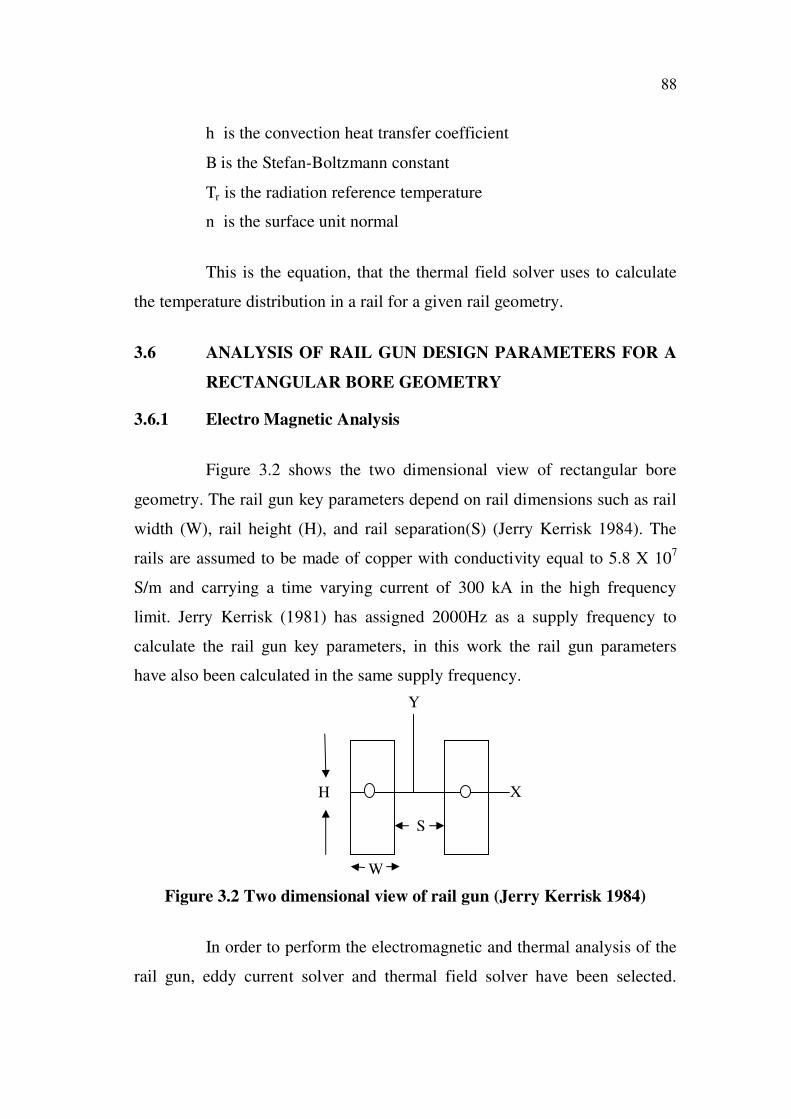
Figure 3.2 shows the two dimensional view of rectangular bore
geometry. The rail gun key parameters depend on rail dimensions such as rail
width (W), rail height (H), and rail separation(S) (Jerry Kerrisk 1984). The
rails are assumed to be made of copper with conductivity equal to 5.8 X 10⁷
S/m and carrying a time varying current of 300 kA in the high frequency
limit. Jerry Kerrisk (1981) has assigned 2000Hz as a supply frequency to
calculate the rail gun key parameters, in this work the rail gun parameters
have also been calculated in the same supply frequency.
Figure 3.2 Two dimensional view of rail gun (Jerry Kerrisk 1984)
In order to perform the electromagnetic and thermal analysis of the
rail gun, eddy current solver and thermal field solver have been selected.
Y
W
+ X
S
H
89
Eddy current field solver is used to calculate the current density distribution,
magnetic flux density between the rails, inductance gradient of the rails, and
repulsive force acting on the rails. Thermal field solver is used to calculate the
temperature distribution over a rail cross section. In order make a trade off
study for rail gun key parameters, rail dimensions are varied. Different values
of W/H and S/H of rail dimensions are taken for modelling the rails. The
value of S/H is varied from 0.25 to 1 in steps of 0.25 and the value of W/H is
varied from 0.1 to 1 in steps of 0.1, and the rail gun parameters are calculated.
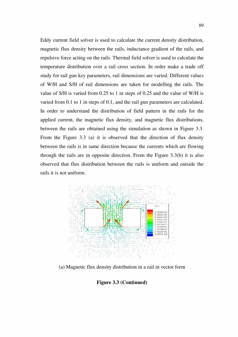
In order to understand the distribution of field pattern in the rails for the
applied current, the magnetic flux density, and magnetic flux distributions,
between the rails are obtained using the simulation as shown in Figure 3.3.
From the Figure 3.3 (a) it is observed that the direction of flux density
between the rails is in same direction because the currents which are flowing
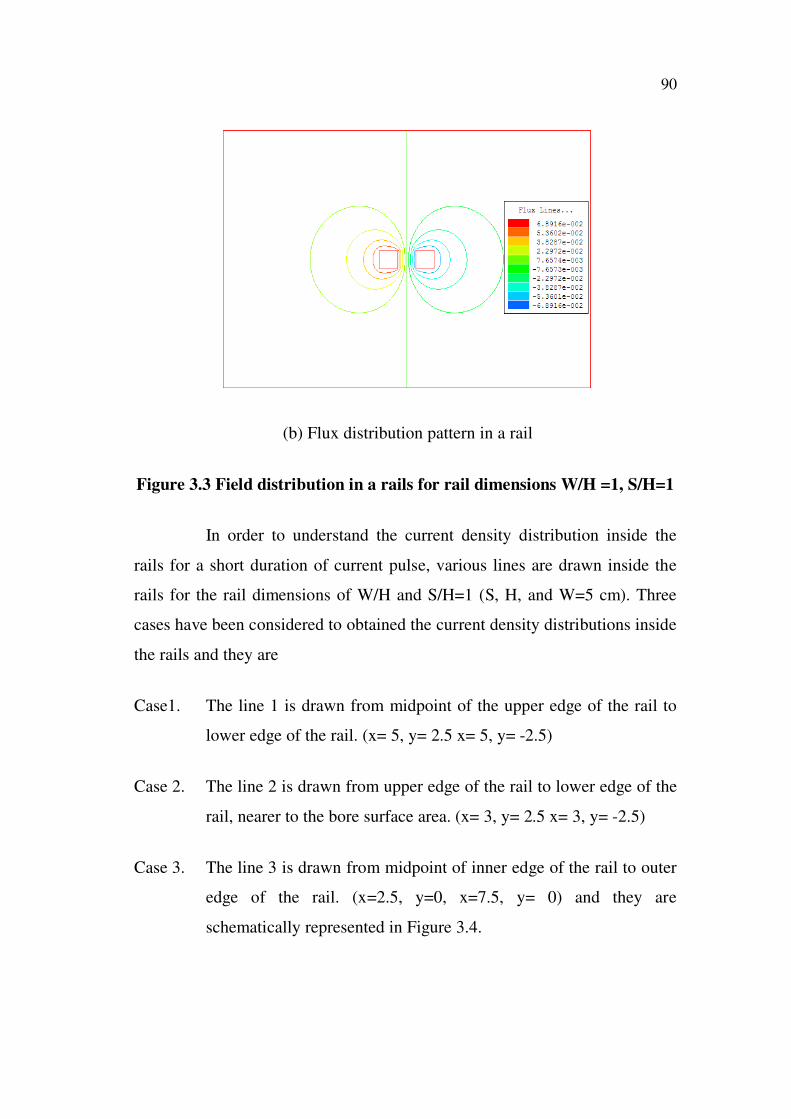
through the rails are in opposite direction. From the Figure 3.3(b) it is also
observed that flux distribution between the rails is uniform and outside the
rails it is not uniform.
(a) Magnetic flux density distribution in a rail in vector form
Figure 3.3 (Continued)
90
(b) Flux distribution pattern in a rail
Figure 3.3 Field distribution in a rails for rail dimensions W/H =1, S/H=1
In order to understand the current density distribution inside the
rails for a short duration of current pulse, various lines are drawn inside the
rails for the rail dimensions of W/H and S/H=1 (S, H, and W=5 cm). Three
cases have been considered to obtained the current density distributions inside
the rails and they are
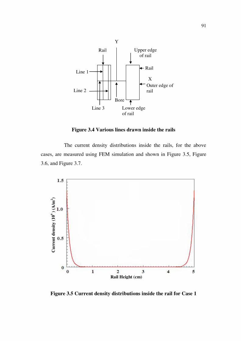
Case1. The line 1 is drawn from midpoint of the upper edge of the rail to
lower edge of the rail. (x= 5, y= 2.5 x= 5, y= -2.5)
Case 2. The line 2 is drawn from upper edge of the rail to lower edge of the
rail, nearer to the bore surface area. (x= 3, y= 2.5 x= 3, y= -2.5)
Case 3. The line 3 is drawn from midpoint of inner edge of the rail to outer
edge of the rail. (x=2.5, y=0, x=7.5, y= 0) and they are
schematically represented in Figure 3.4.
91
Lower edge
of rail
Line 1
Line 2
Line 3
Y
X
Outer edge of
rail
Bore
Rail
Rail
Upper edge
of rail
Figure 3.4 Various lines drawn inside the rails
The current density distributions inside the rails, for the above
cases, are measured using FEM simulation and shown in Figure 3.5, Figure
3.6, and Figure 3.7.
Figure 3.5 Current density distributions inside the rail for Case 1
Cu
rren
t d
ensi
ty (
10
9 )
(A
/m2)
Rail Height (cm)
92
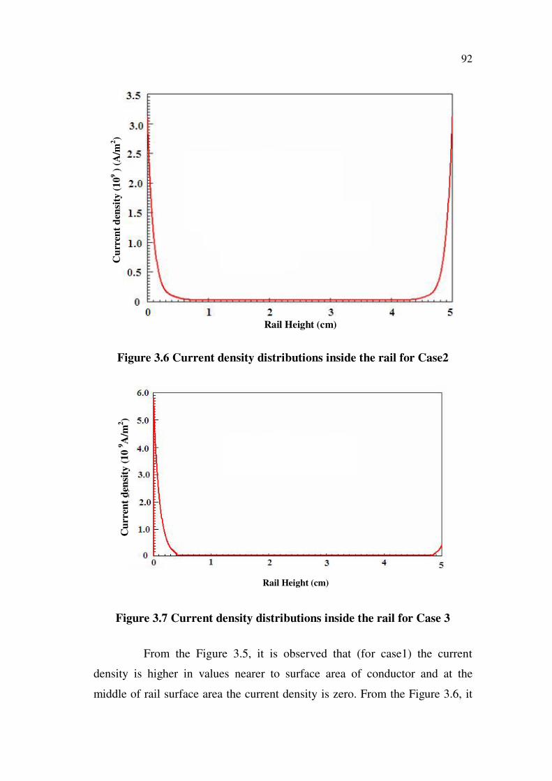
Figure 3.6 Current density distributions inside the rail for Case2
Cu
rren
t d
ensi
ty (
10
9A
/m2)
Rail Height (m)
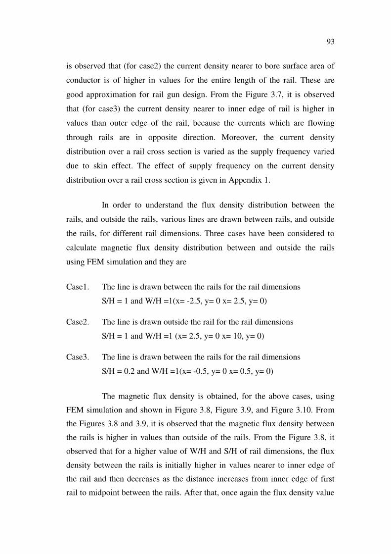
Figure 3.7 Current density distributions inside the rail for Case 3
From the Figure 3.5, it is observed that (for case1) the current
density is higher in values nearer to surface area of conductor and at the
middle of rail surface area the current density is zero. From the Figure 3.6, it
Cu
rren
t d
ensi
ty (
10
9 )
(A
/m2)
Rail Height (cm)
Rail Height (cm)
93
is observed that (for case2) the current density nearer to bore surface area of
conductor is of higher in values for the entire length of the rail. These are
good approximation for rail gun design. From the Figure 3.7, it is observed
that (for case3) the current density nearer to inner edge of rail is higher in
values than outer edge of the rail, because the currents which are flowing
through rails are in opposite direction. Moreover, the current density
distribution over a rail cross section is varied as the supply frequency varied
due to skin effect. The effect of supply frequency on the current density
distribution over a rail cross section is given in Appendix 1.
In order to understand the flux density distribution between the
rails, and outside the rails, various lines are drawn between rails, and outside
the rails, for different rail dimensions. Three cases have been considered to
calculate magnetic flux density distribution between and outside the rails
using FEM simulation and they are
Case1. The line is drawn between the rails for the rail dimensions
S/H = 1 and W/H =1(x= -2.5, y= 0 x= 2.5, y= 0)
Case2. The line is drawn outside the rail for the rail dimensions
S/H = 1 and W/H =1 (x= 2.5, y= 0 x= 10, y= 0)
Case3. The line is drawn between the rails for the rail dimensions
S/H = 0.2 and W/H =1(x= -0.5, y= 0 x= 0.5, y= 0)
The magnetic flux density is obtained, for the above cases, using
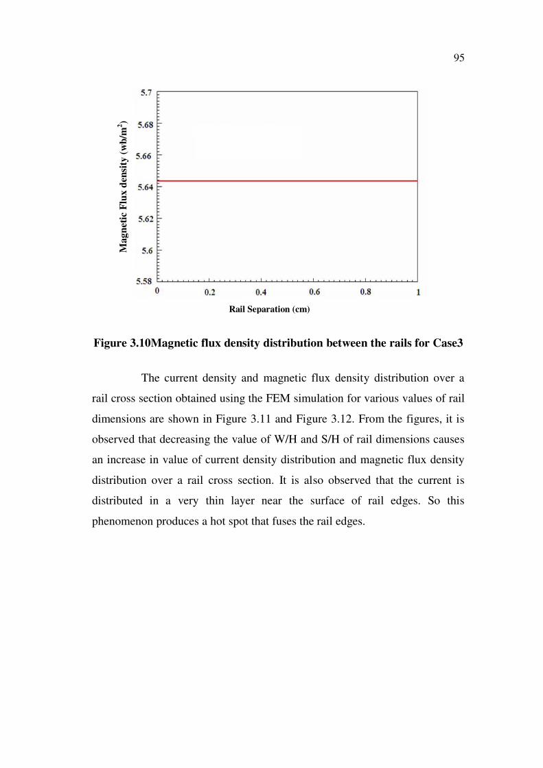
FEM simulation and shown in Figure 3.8, Figure 3.9, and Figure 3.10. From
the Figures 3.8 and 3.9, it is observed that the magnetic flux density between
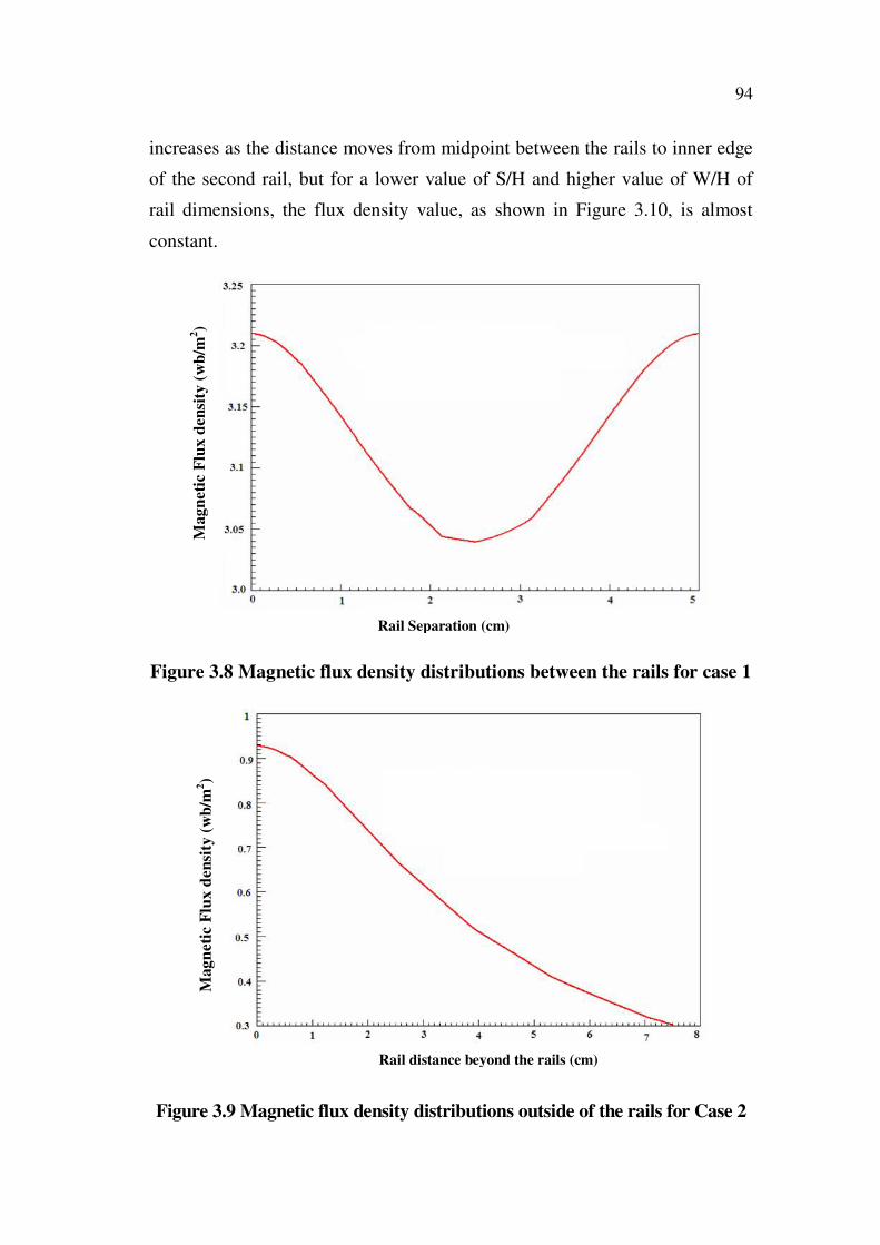
the rails is higher in values than outside of the rails. From the Figure 3.8, it
observed that for a higher value of W/H and S/H of rail dimensions, the flux
density between the rails is initially higher in values nearer to inner edge of
the rail and then decreases as the distance increases from inner edge of first
rail to midpoint between the rails. After that, once again the flux density value
94
increases as the distance moves from midpoint between the rails to inner edge
of the second rail, but for a lower value of S/H and higher value of W/H of
rail dimensions, the flux density value, as shown in Figure 3.10, is almost
constant.
Ma
gn
etic
Flu
x d
ensi
ty (
T)
Rail Separation (m)
Figure 3.8 Magnetic flux density distributions between the rails for case 1
Magn
etic
Flu
x d
ensi
ty (
T)
Rail distance beyond the rails (m)
Figure 3.9 Magnetic flux density distributions outside of the rails for Case 2
Mag
net
ic F
lux
den
sity
(w
b/m
2)
Mag
net
ic F
lux
den
sity
(w
b/m
2)
Rail Separation (cm)
Rail distance beyond the rails (cm)
95
Ma
gn
etic
Flu
xd
ensi
ty (
T)
Rail Separation (m)
Figure 3.10Magnetic flux density distribution between the rails for Case3
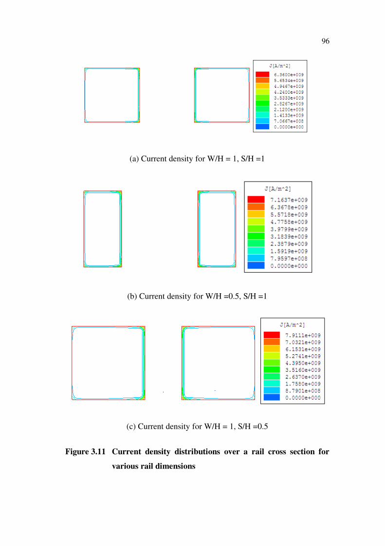
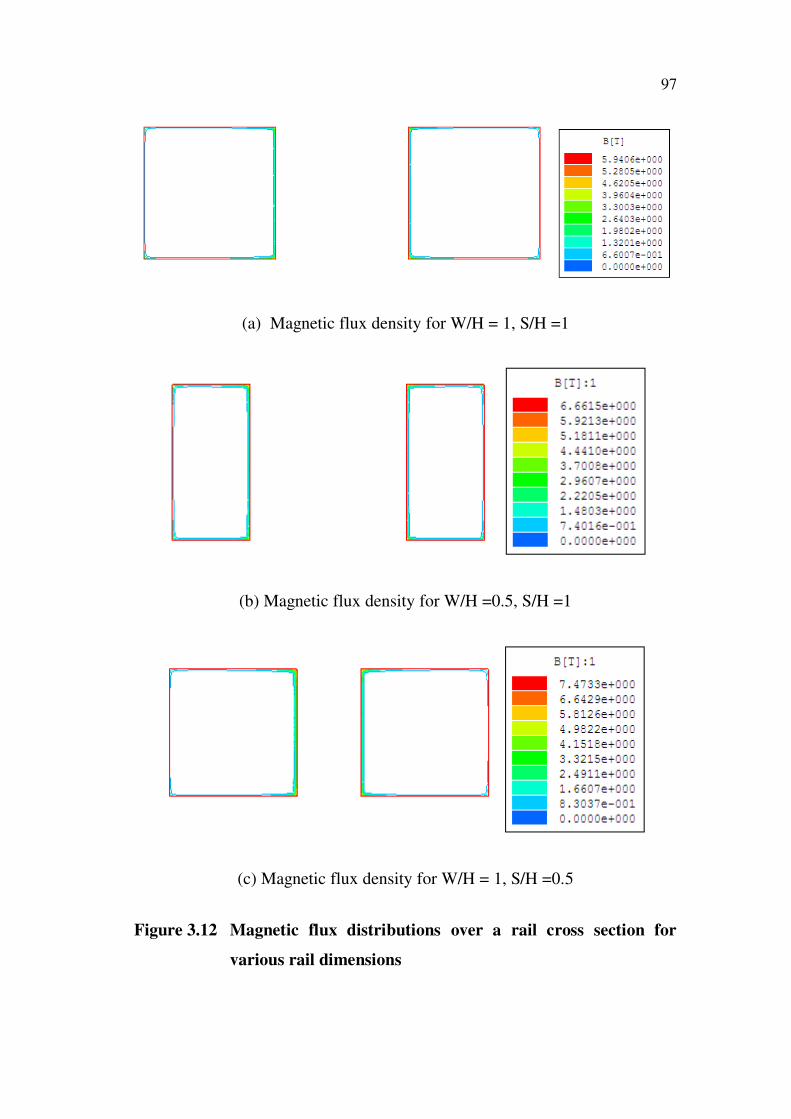
The current density and magnetic flux density distribution over a
rail cross section obtained using the FEM simulation for various values of rail
dimensions are shown in Figure 3.11 and Figure 3.12. From the figures, it is
observed that decreasing the value of W/H and S/H of rail dimensions causes
an increase in value of current density distribution and magnetic flux density
distribution over a rail cross section. It is also observed that the current is
distributed in a very thin layer near the surface of rail edges. So this
phenomenon produces a hot spot that fuses the rail edges.
Mag
net
ic F
lux
den
sity
(w
b/m
2)
Rail Separation (cm)
96
(a) Current density for W/H = 1, S/H =1
(b) Current density for W/H =0.5, S/H =1
(c) Current density for W/H = 1, S/H =0.5
Figure 3.11 Current density distributions over a rail cross section for
various rail dimensions
97
(a) Magnetic flux density for W/H = 1, S/H =1
(b) Magnetic flux density for W/H =0.5, S/H =1
(c) Magnetic flux density for W/H = 1, S/H =0.5
Figure 3.12 Magnetic flux distributions over a rail cross section for
various rail dimensions
98
The L’ values obtained using FEM simulation A.C method in the
high frequency limit, for different rail dimensions, are compared with other
researcher’s values and given in Table 3.1. From the Table 3.1, it is observed
that the L’ values obtained using FEM simulation shows a good agreement
with other researcher’s values. In general, the L’ values varies with respect to
supply frequency. The effect of frequency on L’ values of the rail is given
Appendix1
Table 3.1 Comparison of L’ with other researchers
S.
No
Rail
dimensions
L’ from
Ansoft field
simulator
(µH/m)
Methodology
adopted
L’ from
literature
review
(µH/m)
Methodology
adopted
1 S/H = 1,
W/H = 1
0.4519 FEM analysis
in the high
frequency
limit
0.45174
(Kerrisk 1984)
FDM, A.C in
the high
frequency limit
2 S/H = 1 ,
W/H = 1
0.4519 do 0.45174
(Asghar
Keshtkar 2005)
Transient
analysis
3 S/H = 1 ,
W/H = 0.5
0.3643 do 0.364
(Huerta et al
1991)
Conformal
mapping, A.C
in the high
frequency limit
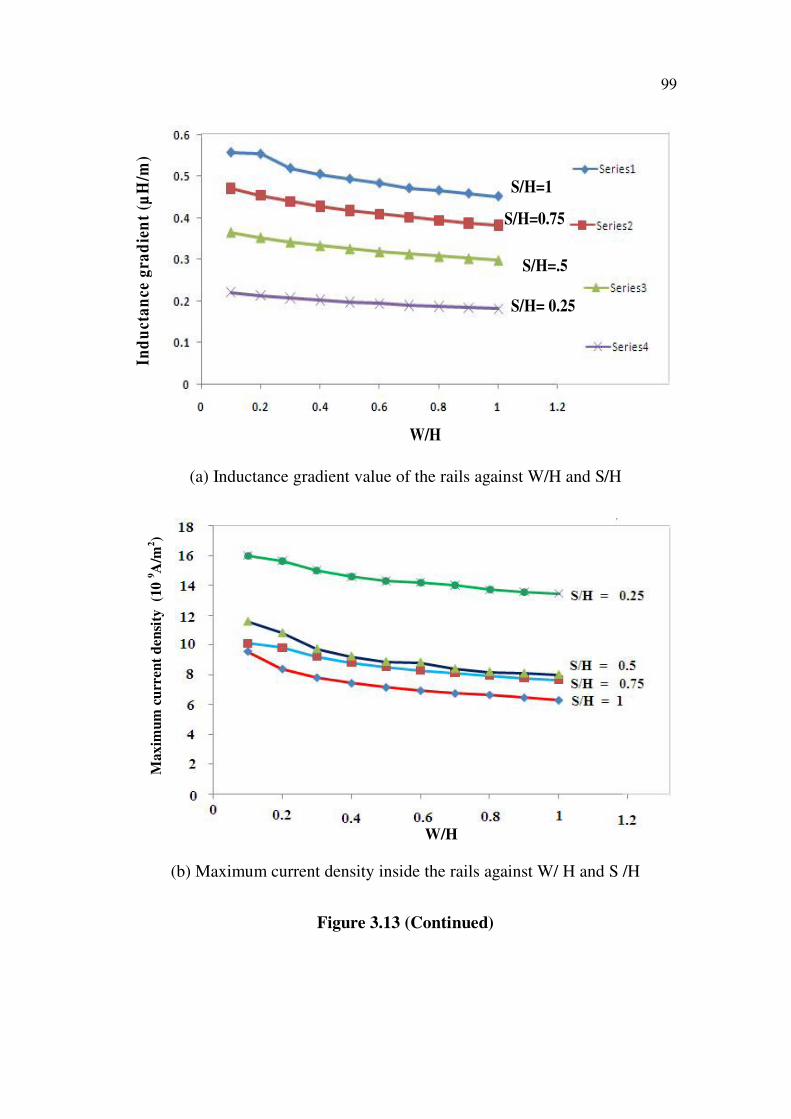
The calculated values of inductance gradient, magnetic flux
density, maximum current density over a rail cross section, and repulsive
force acting on the rails, for various values of W/H and S/H ratios of rail
dimensions are plotted and shown in Figure 3.13.
From the Figure 3.13(a), it is observed that the inductance
gradient values increases with an increase in values of S/H and
decrease in values of W/H of rail dimensions. It is also observed
that the inductance gradient values increases weakly as the
values of W/H varies from 0.5 to 1 and the values of S/H varies
from 0.75 to 1.
99
W/H
Ind
uct
an
ceg
rad
ien
t (µ
H/m
)
S/H=1
S/H=0.75
S/H=.5
S/H= 0.25
(a) Inductance gradient value of the rails against W/H and S/H
Max
imu
m c
urr
en
t d
en
sity
(1
09A
/m2)
W/H
(b) Maximum current density inside the rails against W/ H and S /H
Figure 3.13 (Continued)
100
Magn
etic
Flu
x d
ensi
ty (
T)
W/H
(c) Magnetic flux density between the rails against W/H and S/H
W/H
Rep
uls
ive
forc
e act
ing o
n t
he
rail
s (1
05 N
)
(d) Repulsive force acting on the rails against W/H and S/H
Figure 3.13 Rail gun key parameter values for different rail dimensions
Mag
net
ic F
lux
den
sity
(w
b/m
2)
101
Hence, it is recommended not to vary the values of W/H and
S/H above these ranges in a rail gun design , because in these
ranges, the inductance gradient values increases weakly, since
the force acting on the projectile is proportional to the
inductance gradient of the rails and mass of the projectile, if the
value of W/H varied above these ranges the weight of the rails
will be increased and if the value of S/H varied above these
ranges mass of the projectile will be increased and thereby
making the performance of rail gun poor.
From the Figures 3.13(b), 3.13(c), and 3.13(d), it is observed
that the value of maximum current density over a rail cross
section, magnetic flux density between the rails, and repulsive
force acting on the rails increases as the values of W/H and S/H
decreases.
Hence, the optimum value of W/H is less than 0.5 and that of S/H is
less than 0.75 for rectangular bore geometry. But in these ranges the
maximum value of current density and repulsive force acting on the rails are
very high. Therefore, highly tensile materials with very high conductivity
have to be chosen in these ranges.
3.6.2 Thermal Analysis
In order to perform thermal analysis for a given rail geometry
thermal field solver has been chosen. Eddy current solver is used to assign the
thermal source to the rails. It gives the electromagnetic losses that occur in the
rails due to the ohmic resistance of the rails. These losses are then coupled
with thermal field solver and the temperature distribution inside the rails is
calculated. The thermal conductivity of the rails is assumed as 400 W/m-K
102
and melting point of the rails is assumed as 1084.62 degree centigrade
(Kerrisk 1981). The surface temperature of the rails is assumed as room
temperature (27 C). The surrounding medium of the rails assumed as air
medium and it is assumed that it has the thermal conductivity of 0.026
W/m-K. Simple graphical representation of Electro-Thermal coupled rail gun
model is shown in Figure 3.14. Generally, the thermal conductivity, electrical
conductivity of the rails depends on temperature rise in the rails. In this work,
the value of electrical conductivity and thermal conductivity are assumed to
be independent of temperature.
W
EM
Lo
ss
27oC
Y
X
S
H
EM
Lo
ss
27oC
Figure 3.14 Cross section of Electro Thermal coupled model of the rails
Using the eddy current field solver, the electromagnetic losses that
occur inside the rails due to ohmic heat, is obtained for different rail
dimensions. In order to understand the distribution of electromagnetic losses
that occur inside the rails, a line is drawn from midpoint of the inner edge of
the rail to outer edge of the rail and its value is obtained using the simulation
as shown in Figure 3.15. From the figure, it is observed that the EM losses are
higher in values nearer to the inner edge of the rail than outer edge of the rail.
It is also observed that EM losses are higher in values nearer to the surface
area of conductor and at middle of the rails there is no EM loss. This is due to
that, the nature of the current density distribution inside the rails.
103
Ele
ctro
magnetic loss
(W
/m)
Rail width (m)
Figure 3.15 Electromagnetic loss distributions inside the rail as line
drawn from midpoint of inner edge to outer edge of the rail
The electromagnetic losses that occur in the rails obtained using
simulation for various values of W/H and S/H of rail dimensions are shown in
Figure 3.16. From the Figure, it is observed that decreasing the value of W/H
and S/H of rail dimensions causes an increase in values of electromagnetic
losses that occurs in rails. Moreover, the electromagnetic losses, at corner of
rails, are higher in values than middle of the rails. These losses are coupled
with thermal field solver and then temperature distribution in the rails is
calculated. The temperature distribution over a rail cross-section obtained
using simulation, for various rail dimensions as shown in Figure 3.17. From
the figure, it is observed that temperature values, particularly, that are high
nearer to corners of rails, where the magnetic flux density and current density
are large. It is also observed that the magnitude has higher values at inner
edge of the rail than outer edge. This difference in results is because of the
currents, which flows through rails in opposite direction. It is also observed
that the temperature values inside the rails increases as the values of W/H and
S/H of rail dimensions decreases.
Rail Width (cm)
104
(a) EM loss for W/H =1, S/H =1
(b) EM loss for W/H =0 .5, S/H =1
(c) EM loss for W/H =1, S/H =0.5
Figure 3.16 Distribution of EM losses inside the rails for various rail
dimensions
105
(a) Temperature distribution for W/H =1, S/H =1
(b) Temperature distribution for W/H =0.5, S/H =1
(c) Temperature distribution for W/H =1, S/H =0.5
Figure 3.17 Temperature distributions inside the rails for various rail
dimensions
106
Tem
per
atu
re (
C)
W/H
Figure 3.18 Temperature distributions inside a rail for various rail
dimensions against W/H and S/H
Figure 3.18 shows the maximum values of temperature inside a rail
for various rail dimensions obtained using simulation. It depicts clearly that as
the values of W/H and S/H decreases, the values of temperature inside the
rails increases. It is also observed that for lower values of S/H (at 0.25) and
W/H (below 0.2) of rail dimensions, the values of temperature inside the rails
goes above its melting point. It is important here to note that the inductance
gradient values obtained using simulation is independent of the current
supplied to the rail gun. These values will be the same for any current values
which will be supplied to the rails. But the value of magnetic flux density
between the rails, maximum current density inside the rails, and repulsive
force acting on the rails will vary with respect to the magnitude of the current
supplied to rails. So, the calculated values of magnetic flux density, current
density distribution and repulsive force acting on the rails, in this work are
only applicable for 300kA current.
107
3.7 ANALYSIS OF RAIL GUN DESIGN PARAMETERS FOR
CIRCULAR BORE GEOMETRY
3.7.1 Electro Magnetic Analysis
As the rail gun design parameters values depend on barrel design,
circular bore geometry of rails has also been considered to analysis the
performance of rail gun.
Figure 3.19 Two dimensional view of circular bore geometry of rail
Figure 3.19 shows, the 2-D view of circular bore geometry of rail
gun. The rail gun key parameters depend on rail dimensions of a circular bore
geometry such as rail separation (S), rail thickness (T), and opening angle of
the rails( ).The properties of rails assigned is same as rectangular bore
geometry. For a circular bore geometry, different values of T/S, rail
separation (S), and opening angle ( ) of the rails are taken for modeling the
rails. The rail separation is varied from 2cm to 10 cm in steps of 1cm and an
opening angle of rails is varied from 15 to 45 in increments of 15 . The
value of T/S is varied from 0.1 to 1 in steps of 0.1.
S
T
108
The current density distribution, magnetic flux density between the
rails, inductance gradient of the rails and repulsive force acting on the rails are
computed for different value of T/S, S, and opening angle of the rails. In order
to understand the current density distribution inside the rails, an arc is drawn
inside the rails and its value is obtained as shown in Figure 3.20.
Cu
rren
t d
ensi
ty (
10
9A
/m2)
Arc length (m)
Figure 3.20 Current density distributions inside the rails
From the Figure 3.20, it is observed the current density inside the
rails has a higher in values nearer to surface of conductor and at the middle of
rail surface area the current density is zero. This is good approximation for
rail gun design. In order to understand the magnetic flux density distribution
between the rails, a line is drawn between the rails and its value is obtained as
shown in Figure 3.21. From the Figure3.21, it is observed that, the magnetic
flux density between the rails, initially, has a higher in values nearer to inner
edge of the rails and increases as the distance increases from inner edge of
first rail to midpoint between the rails. After that, once again the flux density
Arc length (cm)
109
decreases as distance increases from midpoint between the rails to the inner
edge of second rail. But in the case of rectangular bore geometry, it is vice
versa.
Magnet
ic F
lux d
ensi
ty (T
)
Rail Separation (m)
Figure 3.21 Magnetic flux density distributions between the rails
The current density distribution and magnetic flux density
distribution over a rail cross section obtained using FEM simulation, for
various rail dimensions are shown in the Figure 3.22 and Figure 3.23.
From the figures, Figure 3.22(a) and Figure 3.22 (b), Figure
3.23 (a) and Figure 3.23(b), it is observed that the values of
maximum current density in the rails and the magnetic flux
density between the rails increases with decrease in values of
rail separation, for same value of T/S , and opening angle of
the rails.
Mag
neti
c F
lux d
ensi
ty (
wb
/m2)
Rail Separation (cm)
110
From the figures, Figure 3.22 (a) and Figure 3.22 (d), Figure
3.23 (a) and Figure 3.23 (d), it is observed that the values of
maximum current density in the rails and the magnetic flux
density between the rails increases with an increase in values of
the opening angle of rails, for same value of T/S and rail
separation.
From the figures, Figure 3.22 (a) and Figure 3.22 (c), Figure
3.23 (a) and Figure 3.23(c), it is observed that the values of
maximum current density in the rails and the magnetic flux
density between the rails increases with decrease in values of
T/S, for same value of rail separation and opening angle of the
rails. Moreover, the current density is distributed in a very thin
layer near the surface of rail inner edges. So, this phenomenon
produces a hot spot that fuses the rail edges.
(a) T/S =1, S= 4cm, = 15
Figure 3.22 (Continued)
111
(b) T/S =1, S= 3cm, = 15
(c) T/S =0.5, S= 4cm, = 15
(d) T/S =1, S= 4cm, = 45
Figure 3.22 Current density distributions over a rail cross section for
various rail dimensions
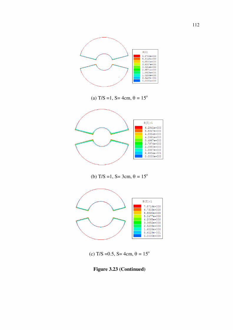
112
(a) T/S =1, S= 4cm, = 15
(b) T/S =1, S= 3cm, = 15
(c) T/S =0.5, S= 4cm, = 15
Figure 3.23 (Continued)
113
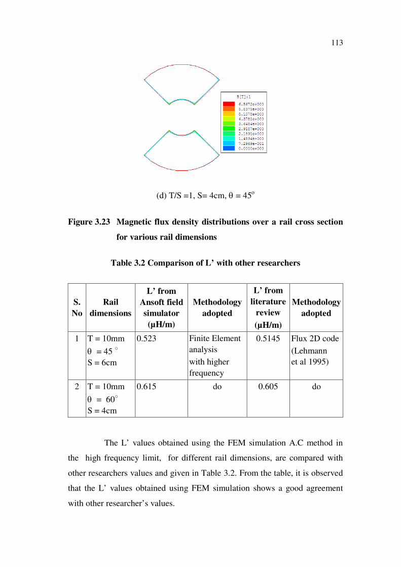
(d) T/S =1, S= 4cm, = 45
Figure 3.23 Magnetic flux density distributions over a rail cross section
for various rail dimensions
Table 3.2 Comparison of L’ with other researchers
S.
No
Rail
dimensions
L’ from
Ansoft field
simulator
(µH/m)
Methodology
adopted
L’ from
literature
review
(µH/m)
Methodology
adopted
1 T = 10mm
= 45
S = 6cm
0.523 Finite Element
analysis
with higher
frequency
0.5145 Flux 2D code
(Lehmann
et al 1995)
2 T = 10mm
= 60
S = 4cm
0.615 do 0.605 do
The L’ values obtained using the FEM simulation A.C method in
the high frequency limit, for different rail dimensions, are compared with
other researchers values and given in Table 3.2. From the table, it is observed
that the L’ values obtained using FEM simulation shows a good agreement
with other researcher’s values.
114
Ind
uct
an
ce g
rad
ien
t (µ
H/m
)
T/S
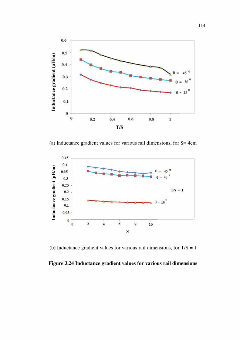
(a) Inductance gradient values for various rail dimensions, for S= 4cm
Ind
uct
an
ce g
rad
ien
t (µ
H/m
)
S
(b) Inductance gradient values for various rail dimensions, for T/S = 1
Figure 3.24 Inductance gradient values for various rail dimensions
115
Ma
gn
etic
Flu
x d
en
sity
(T
)
T/S
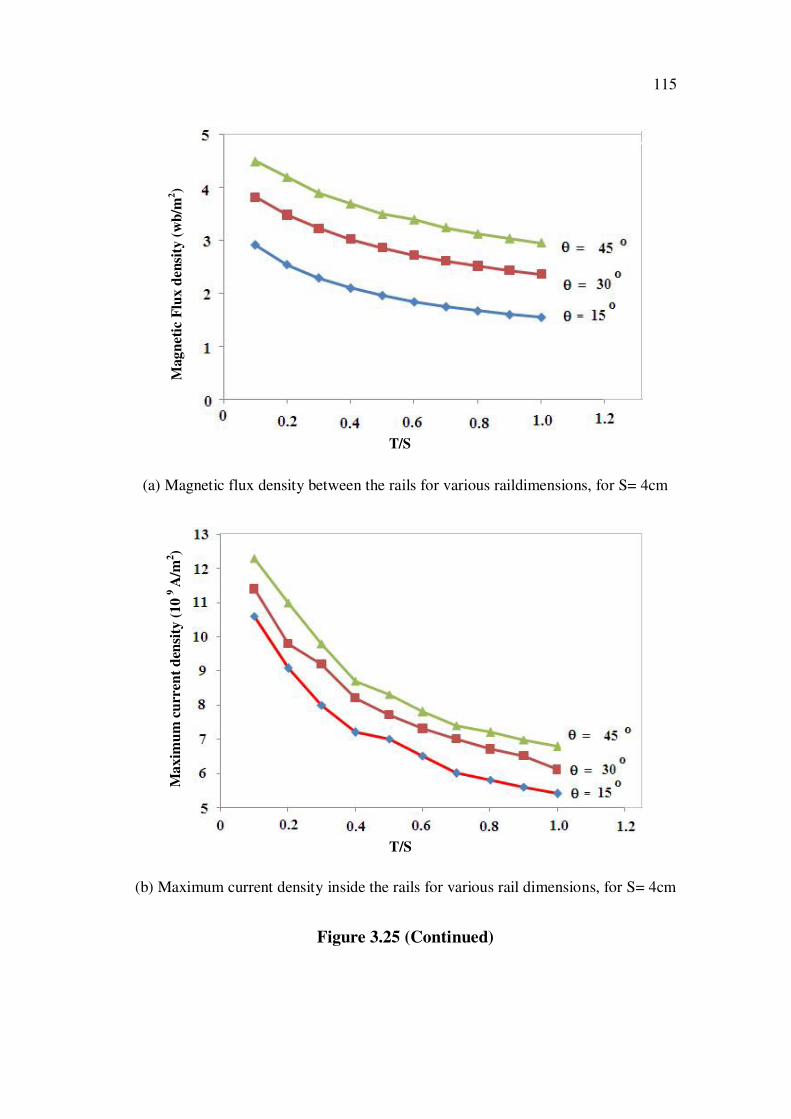
(a) Magnetic flux density between the rails for various raildimensions, for S= 4cm
Maxim
um
cu
rren
t d
ensi
ty (
10
9A
/m2)
T/S
(b) Maximum current density inside the rails for various rail dimensions, for S= 4cm
Figure 3.25 (Continued)
Mag
net
ic F
lux
den
sity
(w
b/m
2)
116
T/S
Rep
uls
ive
force
(10
5 N
)
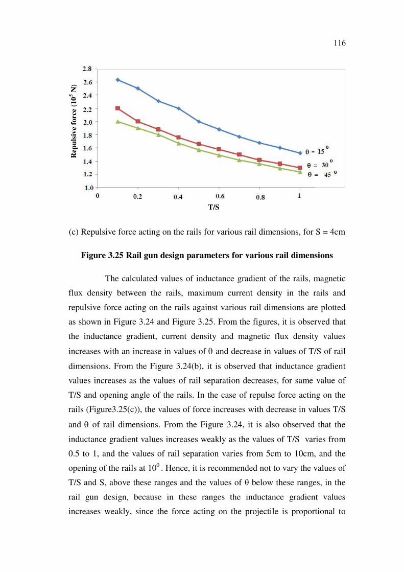
(c) Repulsive force acting on the rails for various rail dimensions, for S = 4cm
Figure 3.25 Rail gun design parameters for various rail dimensions
The calculated values of inductance gradient of the rails, magnetic
flux density between the rails, maximum current density in the rails and
repulsive force acting on the rails against various rail dimensions are plotted
as shown in Figure 3.24 and Figure 3.25. From the figures, it is observed that
the inductance gradient, current density and magnetic flux density values
increases with an increase in values of and decrease in values of T/S of rail
dimensions. From the Figure 3.24(b), it is observed that inductance gradient
values increases as the values of rail separation decreases, for same value of
T/S and opening angle of the rails. In the case of repulse force acting on the
rails (Figure3.25(c)), the values of force increases with decrease in values T/S
and of rail dimensions. From the Figure 3.24, it is also observed that the
inductance gradient values increases weakly as the values of T/S varies from
0.5 to 1, and the values of rail separation varies from 5cm to 10cm, and the
opening of the rails at 100
. Hence, it is recommended not to vary the values of
T/S and S, above these ranges and the values of below these ranges, in the
rail gun design, because in these ranges the inductance gradient values
increases weakly, since the force acting on the projectile is proportional to
117
inductance gradient and mass of the projectile, if the value of T/S varied
above these ranges the weight of the rails will be increased, if the value of
opening angle of rails decreased below these ranges the weight of the rails
will be increased, and if the rail separation value varied above these range the
weight of the projectile will be increased and thereby making the performance
of rail gun poor. Hence, the optimum value of T/S is less than 0.5, for the rail
separation it is less than 5cm and for opening angle of the rails it is above 100,
in order to get better performance of rail gun. But in these ranges the
maximum value of current density and repulsive force acting on the rails are
very high.
3.7.2 Thermal Analysis
In order to obtain the temperature distribution in the rails, using the
eddy current field solver the electromagnetic losses that occurs in rails due to
ohmic heat is obtained for a different rail dimensions. The distribution of EM
losses inside the rails obtained using FEM simulation for the various rail
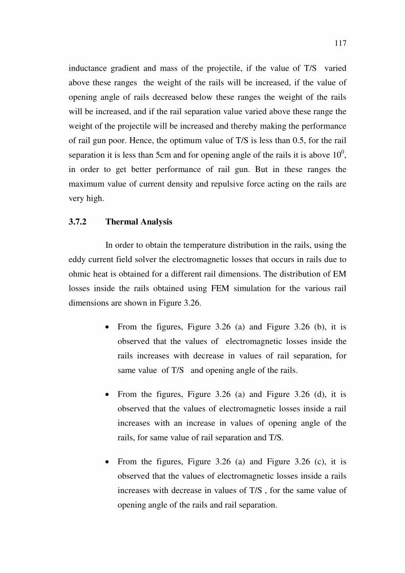
dimensions are shown in Figure 3.26.
From the figures, Figure 3.26 (a) and Figure 3.26 (b), it is
observed that the values of electromagnetic losses inside the
rails increases with decrease in values of rail separation, for
same value of T/S and opening angle of the rails.
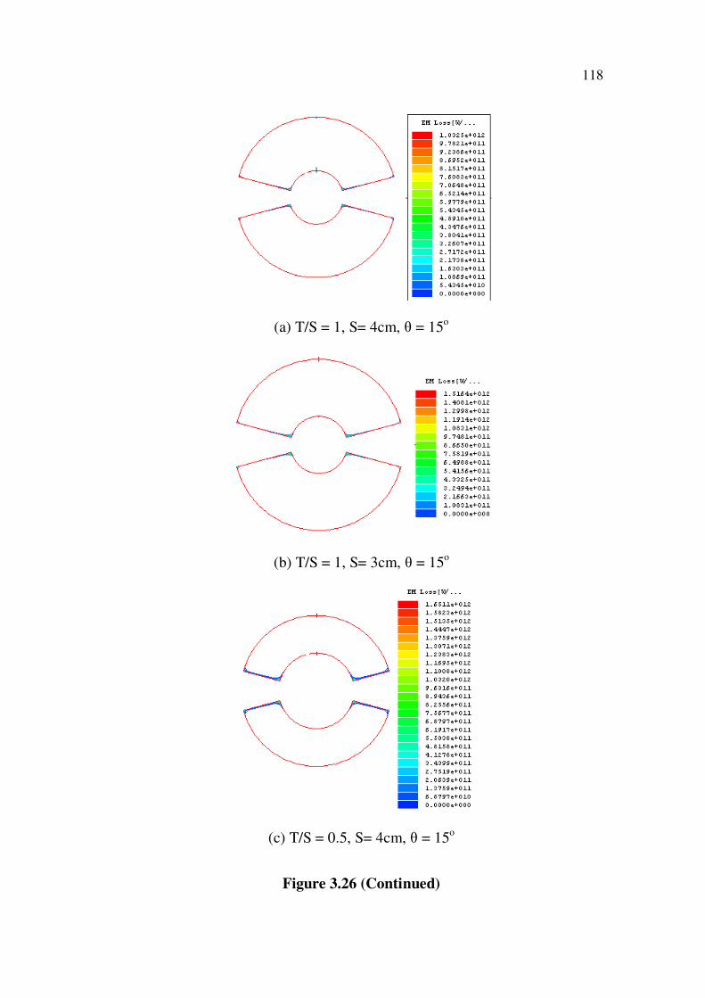
From the figures, Figure 3.26 (a) and Figure 3.26 (d), it is
observed that the values of electromagnetic losses inside a rail
increases with an increase in values of opening angle of the
rails, for same value of rail separation and T/S.
From the figures, Figure 3.26 (a) and Figure 3.26 (c), it is
observed that the values of electromagnetic losses inside a rails
increases with decrease in values of T/S , for the same value of
opening angle of the rails and rail separation.
118
(a) T/S = 1, S= 4cm, = 15o
(b) T/S = 1, S= 3cm, = 15o
(c) T/S = 0.5, S= 4cm, = 15o
Figure 3.26 (Continued)
119
(d) T/S = 1, S= 4cm, = 45o
Figure 3.26 Distribution of electromagnetic losses over a rail cross
section for various rail dimensions
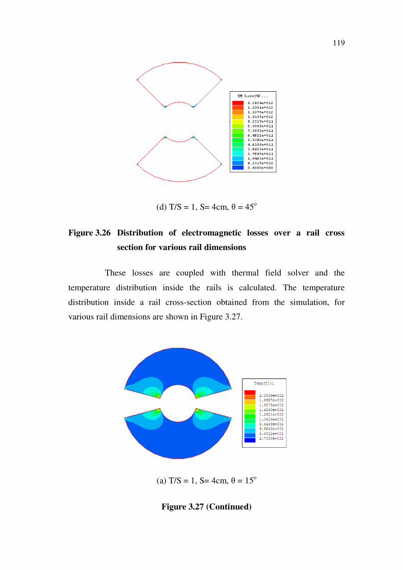
These losses are coupled with thermal field solver and the
temperature distribution inside the rails is calculated. The temperature
distribution inside a rail cross-section obtained from the simulation, for
various rail dimensions are shown in Figure 3.27.
(a) T/S = 1, S= 4cm, = 15o
Figure 3.27 (Continued)
120
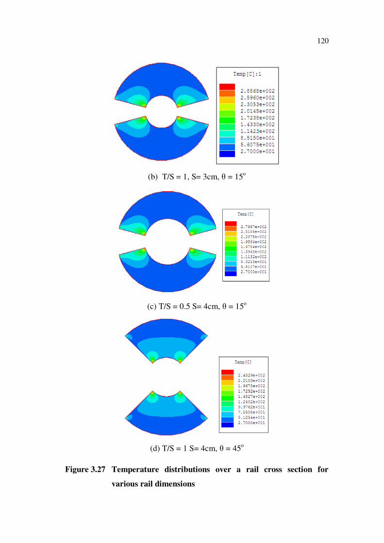
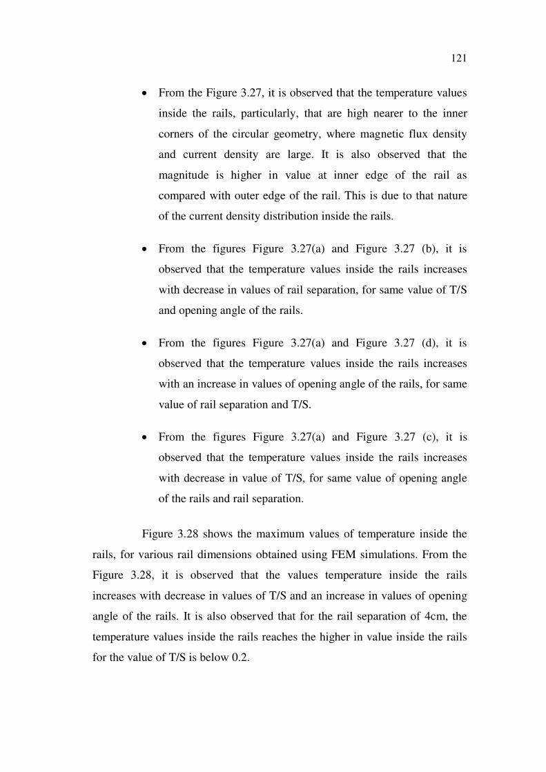
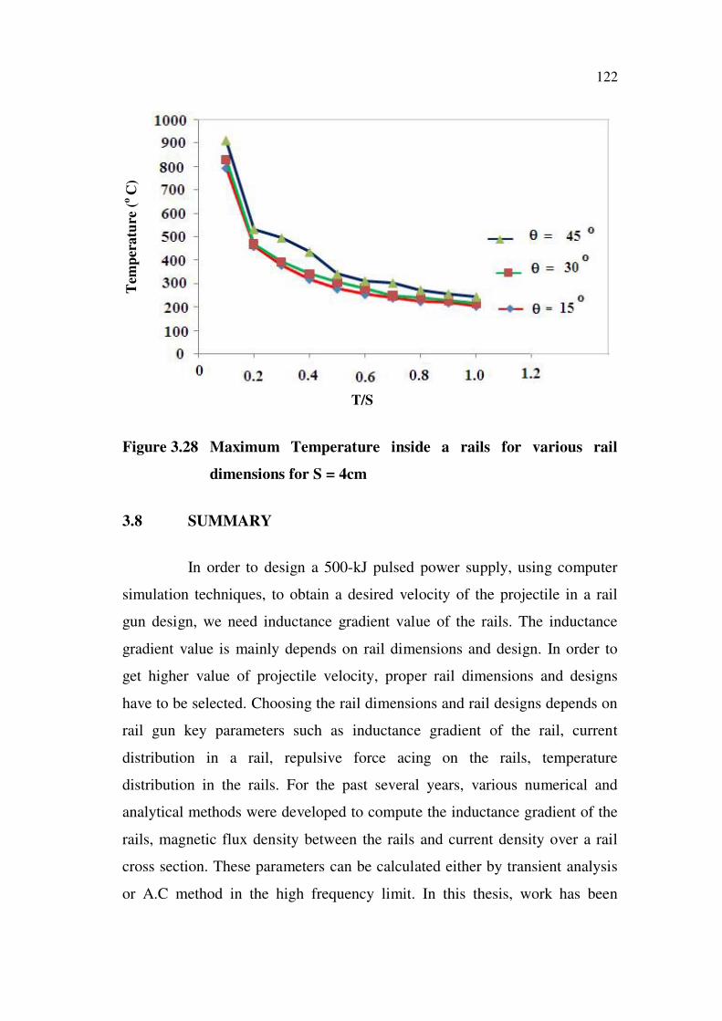
(b) T/S = 1, S= 3cm, = 15o
(c) T/S = 0.5 S= 4cm, = 15o
(d) T/S = 1 S= 4cm, = 45o
Figure 3.27 Temperature distributions over a rail cross section for
various rail dimensions
121
From the Figure 3.27, it is observed that the temperature values
inside the rails, particularly, that are high nearer to the inner
corners of the circular geometry, where magnetic flux density
and current density are large. It is also observed that the
magnitude is higher in value at inner edge of the rail as
compared with outer edge of the rail. This is due to that nature
of the current density distribution inside the rails.
From the figures Figure 3.27(a) and Figure 3.27 (b), it is
observed that the temperature values inside the rails increases
with decrease in values of rail separation, for same value of T/S
and opening angle of the rails.
From the figures Figure 3.27(a) and Figure 3.27 (d), it is
observed that the temperature values inside the rails increases
with an increase in values of opening angle of the rails, for same
value of rail separation and T/S.
From the figures Figure 3.27(a) and Figure 3.27 (c), it is
observed that the temperature values inside the rails increases
with decrease in value of T/S, for same value of opening angle
of the rails and rail separation.
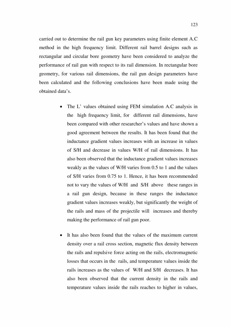
Figure 3.28 shows the maximum values of temperature inside the
rails, for various rail dimensions obtained using FEM simulations. From the
Figure 3.28, it is observed that the values temperature inside the rails
increases with decrease in values of T/S and an increase in values of opening
angle of the rails. It is also observed that for the rail separation of 4cm, the
temperature values inside the rails reaches the higher in value inside the rails
for the value of T/S is below 0.2.
122
Tem
per
atu
re (
C)
T/S
Figure 3.28 Maximum Temperature inside a rails for various rail
dimensions for S = 4cm
3.8 SUMMARY
In order to design a 500-kJ pulsed power supply, using computer
simulation techniques, to obtain a desired velocity of the projectile in a rail
gun design, we need inductance gradient value of the rails. The inductance
gradient value is mainly depends on rail dimensions and design. In order to
get higher value of projectile velocity, proper rail dimensions and designs
have to be selected. Choosing the rail dimensions and rail designs depends on
rail gun key parameters such as inductance gradient of the rail, current
distribution in a rail, repulsive force acing on the rails, temperature
distribution in the rails. For the past several years, various numerical and
analytical methods were developed to compute the inductance gradient of the
rails, magnetic flux density between the rails and current density over a rail
cross section. These parameters can be calculated either by transient analysis
or A.C method in the high frequency limit. In this thesis, work has been
123
carried out to determine the rail gun key parameters using finite element A.C
method in the high frequency limit. Different rail barrel designs such as
rectangular and circular bore geometry have been considered to analyze the
performance of rail gun with respect to its rail dimension. In rectangular bore
geometry, for various rail dimensions, the rail gun design parameters have
been calculated and the following conclusions have been made using the
obtained data’s.
The L’ values obtained using FEM simulation A.C analysis in
the high frequency limit, for different rail dimensions, have
been compared with other researcher’s values and have shown a
good agreement between the results. It has been found that the
inductance gradient values increases with an increase in values
of S/H and decrease in values W/H of rail dimensions. It has
also been observed that the inductance gradient values increases
weakly as the values of W/H varies from 0.5 to 1 and the values
of S/H varies from 0.75 to 1. Hence, it has been recommended
not to vary the values of W/H and S/H above these ranges in
a rail gun design, because in these ranges the inductance
gradient values increases weakly, but significantly the weight of
the rails and mass of the projectile will increases and thereby
making the performance of rail gun poor.
It has also been found that the values of the maximum current
density over a rail cross section, magnetic flux density between
the rails and repulsive force acting on the rails, electromagnetic
losses that occurs in the rails, and temperature values inside the
rails increases as the values of W/H and S/H decreases. It has
also been observed that the current density in the rails and
temperature values inside the rails reaches to higher in values,
124
for the value of W/H is less than 0.5 and value of S/H is greater
than 0.5. Hence, based on the L’ values, in order to get better
performance of rail gun the value S/H would be less than 0.75
and value of W/H would be less than 0.5, but in these ranges the
current density distribution in rail and repulsive force acting on
the rails and temperature distribution in the rails would be
higher in values.
In circular bore geometry for various rail dimensions, the rail gun
design parameters have been calculated and the following conclusions have
been made using the obtained data’s.
The L’ values obtained using FEM simulation A.C analysis in
the high frequency limit, for different rail dimensions have
been compared with other researcher’s values and have shown a
good agreement between the results.
It has been observed that the inductance gradient values
increases with an increase in value of opening angle the rails ,
and decrease in values of T/S of rail dimensions. It has also
been observed that the inductance gradient values increases as
the values of rail separation decreases, for the same value of T/S
and opening angle of the rails. It has also been observed that the
inductance gradient values increases weakly as the values of T/S
varies from 0.5 to 1 and rail separation varies from 5cm to 10cm
and opening angle of the rails at 10 . Hence, it has been
recommended not to vary the value of T/S and S above these
ranges and the opening angle of the rails below 10o, because in
these ranges the inductance gradient values will increases
weakly and thereby making the performance of rail gun poor.
125
It has been found that the values of current density the rails,
magnetic flux density between the rails, electromagnetic losses
that occur inside the rails, and temperature distribution in the
rails increases as the values of T/S , rail separation, and opening
of the rails decreases. It has also been observed that the values
of temperature inside in the rails reaches to higher in values as
the values of T/S below 0.2, when S= 4cm. Hence, based on the
L’ values, in order to get better performance of the rail gun, the
value of T/S would be less than 0.5 and the rail separation
would be less than 5cm and the opening angle of the rails would
be greater than 10o
, but in these ranges the current density
distribution in the rails and repulsive force acting on the rails
and temperature distribution in the rails would be higher in
values. In order to withstand higher value current density and
temperature in the rails, the copper alloy material can be used to
design a rail barrel in rail gun system.
The researchers who analyzed the rail gun key parameters by
varying the rail dimensions (for rectangular bore geometry S, H
and W and for circular bore geometry T, S and ) separately. In
this work, ratios of rail dimensions have been considered to
calculate the rail gun parameters. As the maximum current
supplied by the 500kJ PPS is 300kA, in this work, the
electromagnetic and thermal analysis were made at 300kA
current. Finally an attempt is made to give optimum value of
rail dimensions after calculating the rail gun key parameters. As
the temperature rise in the rails depends on armature shape and
time period, 3–D model have been developed to calculate the
temperature rise in the rails in order to take armature effect and
time period, and the results are given in Appendix2.