CHAPTER 2econ.lse.ac.uk/staff/spischke/ec533/Acemoglu Autor chapter 2.pdf · CHAPTER 2 Human Capital and Signaling 1. The Basic Model of Labor Market Signaling The models we have

CHAPTER 2

Human Capital and Signaling

1. The Basic Model of Labor Market Signaling

The models we have discussed so far are broadly in the tradition of Becker’s

approach to human capital. Human capital is viewed as an input in the production

process. The leading alternative is to view education purely as a signal. Consider

the following simple model to illustrate the issues.

There are two types of workers, high ability and low ability. The fraction of

high ability workers in the population is λ. Workers know their own ability, but

employers do not observe this directly. High ability workers always produce yH ,

while low ability workers produce yL. In addition, workers can obtain education.

The cost of obtaining education is cH for high ability workers and cL for low ability

workers. The crucial assumption is that cL > cH , that is, education is more costly

for low ability workers. This is often referred to as the “single-crossing” assumption,

since it makes sure that in the space of education and wages, the indifference curves

of high and low types intersect only once. For future reference, let us denote the

decision to obtain education by e = 1.

For simplicity, we assume that education does not increase the productivity of

either type of worker. Once workers obtain their education, there is competition

among a large number of risk-neutral firms, so workers will be paid their expected

productivity. More specifically, the timing of events is as follows:

• Each worker finds out their ability.• Each worker chooses education, e = 0 or e = 1.• A large number of firms observe the education decision of each worker (butnot their ability) and compete a la Bertrand to hire these workers.

35

Lectures in Labor Economics

Clearly, this environment corresponds to a dynamic game of incomplete informa-

tion, since individuals know their ability, but firms do not. In natural equilibrium

concept in this case is the Perfect Bayesian Equilibrium. Recall that a Perfect

Bayesian Equilibrium consists of a strategy profile σ (designating a strategy for

each player) and a brief profile μ (designating the beliefs of each player at each

information set) such that σ is sequentially rational for each player given μ (so that

each player plays the best response in each information set given their beliefs) and

μ is derived from σ using Bayes’s rule whenever possible. While Perfect Bayesian

Equilibria are straightforward to characterize and often reasonable, in incomplete

information games where players with private information move before those with-

out this information, there may also exist Perfect Bayesian Equilibria with certain

undesirable characteristics. We may therefore wish to strengthen this notion of

equilibrium (see below).

In general, there can be two types of equilibria in this game.

(1) Separating, where high and low ability workers choose different levels of

schooling, and as a result, in equilibrium, employers can infer worker ability

from education (which is a straightforward application of Bayesian updat-

ing).

(2) Pooling, where high and low ability workers choose the same level of edu-

cation.

In addition, there can be semi-separating equilibria, where some education levels

are chosen by more than one type.

1.1. A separating equilibrium. Let us start by characterizing a possible sep-

arating equilibrium, which illustrates how education can be valued, even though it

has no directly productive role.

Suppose that we have

(2.1) yH − cH > yL > yH − cL

36


This is clearly possible since cH < cL. Then the following is an equilibrium: all high

ability workers obtain education, and all low ability workers choose no education.

Wages (conditional on education) are:

w (e = 1) = yH and w (e = 0) = yL

Notice that these wages are conditioned on education, and not directly on ability,

since ability is not observed by employers. Let us now check that all parties are

playing best responses. First consider firms. Given the strategies of workers (to

obtain education for high ability and not to obtain education for low ability), a

worker with education has productivity yH while a worker with no education has

productivity yL. So no firm can change its behavior and increase its profits.

What about workers? If a high ability worker deviates to no education, he will

obtain w (e = 0) = yL, whereas he’s currently getting w (e = 1)−cH = yH−cH > yL.

If a low ability worker deviates to obtaining education, the market will perceive him

as a high ability worker, and pay him the higher wage w (e = 1) = yH . But from

(2.1), we have that yH − cL < yL, so this deviation is not profitable for a low ability

worker, proving that the separating allocation is indeed an equilibrium.

In this equilibrium, education is valued simply because it is a signal about ability.

Education can be a signal about ability because of the single-crossing property. This

can be easily verified by considering the case in which cL ≤ cH . Then we could never

have condition (2.1) hold, so it would not be possible to convince high ability workers

to obtain education, while deterring low ability workers from doing so.

Notice also that if the game was one of perfect information, that is, the worker

type were publicly observed, there could never be education investments here. This

is an extreme result, due to the assumption that education has no productivity

benefits. But it illustrates the forces at work.

1.2. Pooling equilibria in signaling games. However, the separating equi-

librium is not the only one. Consider the following allocation: both low and high

37


ability workers do not obtain education, and the wage structure is

w (e = 1) = (1− λ) yL + λyH and w (e = 0) = (1− λ) yL + λyH

It is straightforward to check that no worker has any incentive to obtain edu-

cation (given that education is costly, and there are no rewards to obtaining it).

Since all workers choose no education, the expected productivity of a worker with

no education is (1− λ) yL+λyH , so firms are playing best responses. (In Nash Equi-

librium and Perfect Bayesian Equilibrium, what they do in response to a deviation

by a worker who obtains education is not important, since this does not happen

along the equilibrium path).

What is happening here is that the market does not view education as a good

signal, so a worker who “deviates” and obtains education is viewed as an average-

ability worker, not as a high-ability worker.

What we have just described is a Perfect Bayesian Equilibrium. But is it reason-

able? The answer is no. This equilibrium is being supported by the belief that the

worker who gets education is no better than a worker who does not. But education

is more costly for low ability workers, so they should be less likely to deviate to

obtaining education. There are many refinements in game theory which basically

try to restrict beliefs in information sets that are not reached along the equilibrium

path, ensuring that “unreasonable” beliefs, such as those that think a deviation to

obtaining education is more likely from a low ability worker, are ruled out.

Perhaps the simplest is The Intuitive Criterion introduced by Cho and Kreps.

The underlying idea is as follows. If there exists a type who will never benefit

from taking a particular deviation, then the uninformed parties (here the firms)

should deduce that this deviation is very unlikely to come from this type. This

falls within the category of “forward induction” where rather than solving the game

simply backwards, we think about what type of inferences will others derive from a

deviation.

38


To illustrate the main idea, let us simplify the discussion by slightly strengthening

condition (2.1) to

(2.2) yH − cH > (1− λ) yL + λyH and yL > yH − cL.

Now take the pooling equilibrium above. Consider a deviation to e = 1. There is

no circumstance under which the low type would benefit from this deviation, since

by assumption (2.2) we have yL > yH − cL, and the most a worker could ever get is

yH , and the low ability worker is now getting (1− λ) yL+λyH . Therefore, firms can

deduce that the deviation to e = 1 must be coming from the high type, and offer

him a wage of yH . Then (2.2) also ensures that this deviation is profitable for the

high types, breaking the pooling equilibrium.

The reason why this refinement is referred to as “The Intuitive Criterion” is

that it can be supported by a relatively intuitive “speech” by the deviator along the

following lines: “you have to deduce that I must be the high type deviating to e = 1,

since low types would never ever consider such a deviation, whereas I would find

it profitable if I could convince you that I am indeed the high type).” You should

bear in mind that this speech is used simply as a loose and intuitive description of

the reasoning underlying this equilibrium refinement. In practice there are no such

speeches, because the possibility of making such speeches has not been modeled as

part of the game. Nevertheless, this heuristic device gives the basic idea.

The overall conclusion is that as long as the separating condition is satisfied,

we expect the equilibrium of this economy to involve a separating allocation, where

education is valued as a signal.

2. Generalizations

It is straightforward to generalize this equilibrium concept to a situation in which

education has a productive role as well as a signaling role. Then the story would be

one where education is valued for more than its productive effect, because it is also

associated with higher ability.

39


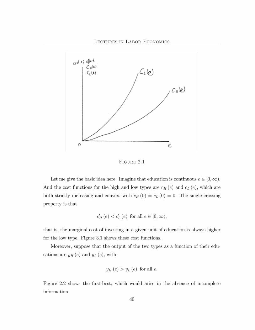
Figure 2.1

Let me give the basic idea here. Imagine that education is continuous e ∈ [0,∞).And the cost functions for the high and low types are cH (e) and cL (e), which are

both strictly increasing and convex, with cH (0) = cL (0) = 0. The single crossing

property is that

c0H (e) < c0L (e) for all e ∈ [0,∞),

that is, the marginal cost of investing in a given unit of education is always higher

for the low type. Figure 3.1 shows these cost functions.

Moreover, suppose that the output of the two types as a function of their edu-

cations are yH (e) and yL (e), with

yH (e) > yL (e) for all e.

Figure 2.2 shows the first-best, which would arise in the absence of incomplete

information.

40


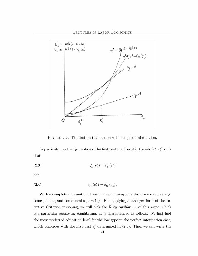
Figure 2.2. The first best allocation with complete information.

In particular, as the figure shows, the first best involves effort levels (e∗l , e∗h) such

that

(2.3) y0L (e∗l ) = c0L (e

∗l )

and

(2.4) y0H (e∗h) = c0H (e

∗h) .

With incomplete information, there are again many equilibria, some separating,

some pooling and some semi-separating. But applying a stronger form of the In-

tuitive Criterion reasoning, we will pick the Riley equilibrium of this game, which

is a particular separating equilibrium. It is characterized as follows. We first find

the most preferred education level for the low type in the perfect information case,

which coincides with the first best e∗l determined in (2.3). Then we can write the

41


incentive compatibility constraint for the low type, such that when the market ex-

pects low types to obtain education e∗l , the low type does not try to mimic the high

type; in other words, the low type agent should not prefer to choose the education

level the market expects from the high type, e, and receive the wage associated with

this level of education. This incentive compatibility constraint is straightforward to

write once we note that in the wage level that low type workers will obtain is exactly

yL (e∗l ) in this case, since we are looking at the separating equilibrium. Thus the

incentive compatibility constraint is simply

(2.5) yL (e∗l )− cL (e

∗l ) ≥ w (e)− cL (e) for all e,

where w (e) is the wage rate paid for a worker with education e. Since e∗l is the first-

best effort level for the low type worker, if we had w (e) = yL (e), this constraint

would always be satisfied. However, since the market can not tell low and high type

workers apart, by choosing a different level of education, a low type worker may be

able to “mimic” and high type worker and thus we will typically have w (e) ≥ yL (e)

when e ≥ e∗l , with a strict inequality for some values of education. Therefore, the

separating (Riley) equilibrium must satisfy (2.5) for the equilibrium wage function

w (e).

To make further progress, note that in a separating equilibrium, there will exist

some level of education, say eh, that will be chosen by high type workers. Then,

Bertrand competition among firms, with the reasoning similar to that in the previous

section, implies that w (eh) = yH (eh). Therefore, if a low type worker deviates to

this level of effort, the market will take him to be a high type worker and pay him

the wage yH (eh). Now take this education level eh to be such that the incentive

compatibility constraint, (2.5), holds as an equality, that is,

(2.6) yL (e∗l )− cL (e

∗l ) = yH (eh)− cL (eh) .

Then the Riley equilibrium is such that low types choose e∗l and obtain the wage

w (e∗l ) = yL (e∗l ), and high types choose eh and obtain the wage w (eh) = yH (eh).

That high types are happy to do this follows immediately from the single-crossing

42


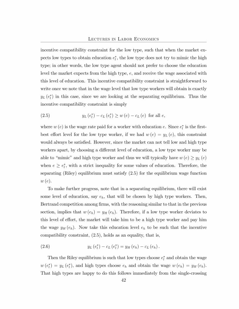
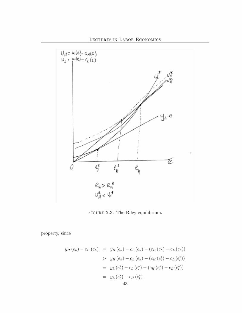
Figure 2.3. The Riley equilibrium.

property, since

yH (eh)− cH (eh) = yH (eh)− cL (eh)− (cH (eh)− cL (eh))

> yH (eh)− cL (eh)− (cH (e∗l )− cL (e∗l ))

= yL (e∗l )− cL (e

∗l )− (cH (e∗l )− cL (e

∗l ))

= yL (e∗l )− cH (e

∗l ) ,

43


where the first line is introduced by adding and subtracting cL (eh). The second line

follows from single crossing, since cH (eh)− cL (eh) < cH (e∗l )− cL (e

∗l ) in view of the

fact that e∗l < eh. The third line exploits (2.6), and the final line simply cancels the

two cL (e∗l ) terms from the right hand side.

Figure 2.3 depicts this equilibrium diagrammatically (for clarity it assumes that

yH (e) and yL (e) are linear in e).

Notice that in this equilibrium, high type workers invest more than they would

have done in the perfect information case, in the sense that eh characterized here

is greater than the education level that high type individuals chosen with perfect

information, given by e∗h in (2.4).

3. Evidence on Labor Market Signaling

Is the signaling role of education important? There are a number of different

ways of approaching this question. Unfortunately, direct evidence is difficult to find

since ability differences across workers are not only unobserved by firms, but also by

econometricians. Nevertheless, number of different strategies can be used to gauge

the importance of signaling in the labor market. Here we will discuss a number of

different attempts that investigate the importance of labor market signaling. In the

next section, we will discuss empirical work that may give a sense of how important

signaling considerations are in the aggregate.

Before this discussion, note the parallel between the selection stories discussed

above and the signaling story. In both cases, the observed earnings differences

between high and low education workers will include a component due to the fact

that the abilities of the high and low education groups differ. There is one important

difference, however, in that in the selection stories, the market observed ability, it

was only us, the economists or the econometricians, who were unable to do so. In

the signaling story, the market is also unable to observed ability, and is inferring

it from education. For this reason, proper evidence in favor of the signaling story

should go beyond documenting the importance of some type of “selection”.

44


There are four different approaches to determining whether signaling is impor-

tant. The first line of work looks at whether degrees matter, in particular, whether

a high school degree or the fourth year of college that gets an individual a university

degree matter more than other years of schooling (e.g., Kane and Rouse). This

approach suffers from two serious problems. First, the final year of college (or high

school) may in fact be more useful than the third-year, especially because it shows

that the individual is being able to learn all the required information that makes up

a college degree. Second, and more serious, there is no way of distinguishing selec-

tion and signaling as possible explanations for these patterns. It may be that those

who drop out of high school are observationally different to employers, and hence

receive different wages, but these differences are not observed by us in the standard

data sets. This is a common problem that will come back again: the implications

of unobserved heterogeneity and signaling are often similar.

Second, a creative paper by Lang and Kropp tests for signaling by looking at

whether compulsory schooling laws affect schooling above the regulated age. The

reasoning is that if the 11th year of schooling is a signal, and the government legis-

lates that everybody has to have 11 years of schooling, now high ability individuals

have to get 12 years of schooling to distinguish themselves. They find evidence for

this, which they interpret as supportive of the signaling model. The problem is that

there are other reasons for why compulsory schooling laws may have such effects.

For example, an individual who does not drop out of 11th grade may then decide to

complete high school. Alternatively, there can be peer group effects in that as fewer

people drop out of school, it may become less socially acceptable the drop out even

at later grades.

The third approach is the best. It is pursued in a very creative paper by Tyler,

Murnane and Willett. They observe that passing grades in the Graduate Equivalent

Degree (GED) differ by state. So an individual with the same grade in the GED

exam will get a GED in one state, but not in another. If the score in the exam is an

unbiased measure of human capital, and there is no signaling, these two individuals

45


should get the same wages. In contrast, if the GED is a signal, and employers do

not know where the individual took the GED exam, these two individuals should

get different wages.

Using this methodology, the authors estimate that there is a 10-19 percent return

to a GED signal. The attached table shows the results.

An interesting result that Tyler, Murnane and Willett find is that there are

no GED returns to minorities. This is also consistent with the signaling view,

since it turns out that many minorities prepare for and take the GED exam in

prison. Therefore, GED would not only be a positive signal about ability, but also

potentially a signal that the individual was at some point incarcerated. This latter

feature makes a GED less of that positive signal for minorities.

46

CHAPTER 3

Externalities and Peer Effects

Many economists believe that human capital not only creates private returns,

increasing the earnings of the individual who acquires it, but it also creates external-

ities, i.e., it increases the productivity of other agents in the economy (e.g., Jacobs,

Lucas). If so, existing research on the private returns to education is only part of the

picture–the social return, i.e., the private return plus the external return, may far

exceed the private return. Conversely, if signaling is important, the private return

overestimates the social return to schooling. Estimating the external and the social

returns to schooling is a first-order question.

1. Theory

To show how and why external returns to education may arise, we will briefly

discuss two models. The first is a theory of non-pecuniary external returns, meaning

that external returns arise from technological linkages across agents or firms. The

second is pecuniary model of external returns, thus externalities will arise from mar-

ket interactions and changes in market prices resulting from the average education

level of the workers.

1.1. Non-pecuniary human capital externalities. Suppose that the output

(or marginal product) of a worker, i, is

yi = Ahνi ,

where hi is the human capital (schooling) of the worker, and A is aggregate pro-

ductivity. Assume that labor markets are competitive. So individual earnings are

Wi = Ahνi .

47


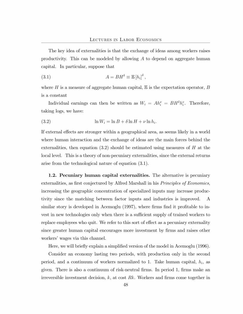
The key idea of externalities is that the exchange of ideas among workers raises

productivity. This can be modeled by allowing A to depend on aggregate human

capital. In particular, suppose that

(3.1) A = BHδ ≡ E [hi]δ ,

where H is a measure of aggregate human capital, E is the expectation operator, Bis a constant

Individual earnings can then be written as Wi = Ahνi = BHδhvi . Therefore,

taking logs, we have:

(3.2) lnWi = lnB + δ lnH + ν lnhi.

If external effects are stronger within a geographical area, as seems likely in a world

where human interaction and the exchange of ideas are the main forces behind the

externalities, then equation (3.2) should be estimated using measures of H at the

local level. This is a theory of non-pecuniary externalities, since the external returns

arise from the technological nature of equation (3.1).

1.2. Pecuniary human capital externalities. The alternative is pecuniary

externalities, as first conjectured by Alfred Marshall in his Principles of Economics,

increasing the geographic concentration of specialized inputs may increase produc-

tivity since the matching between factor inputs and industries is improved. A

similar story is developed in Acemoglu (1997), where firms find it profitable to in-

vest in new technologies only when there is a sufficient supply of trained workers to

replace employees who quit. We refer to this sort of effect as a pecuniary externality

since greater human capital encourages more investment by firms and raises other

workers’ wages via this channel.

Here, we will briefly explain a simplified version of the model in Acemoglu (1996).

Consider an economy lasting two periods, with production only in the second

period, and a continuum of workers normalized to 1. Take human capital, hi, as

given. There is also a continuum of risk-neutral firms. In period 1, firms make an

irreversible investment decision, k, at cost Rk. Workers and firms come together in

48


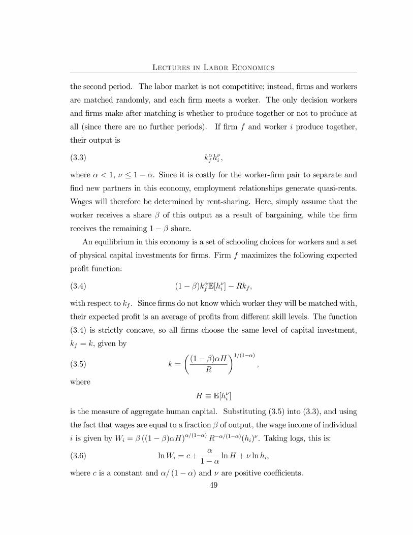
the second period. The labor market is not competitive; instead, firms and workers

are matched randomly, and each firm meets a worker. The only decision workers

and firms make after matching is whether to produce together or not to produce at

all (since there are no further periods). If firm f and worker i produce together,

their output is

(3.3) kαf hνi ,

where α < 1, ν ≤ 1− α. Since it is costly for the worker-firm pair to separate and

find new partners in this economy, employment relationships generate quasi-rents.

Wages will therefore be determined by rent-sharing. Here, simply assume that the

worker receives a share β of this output as a result of bargaining, while the firm

receives the remaining 1− β share.

An equilibrium in this economy is a set of schooling choices for workers and a set

of physical capital investments for firms. Firm f maximizes the following expected

profit function:

(3.4) (1− β)kαfE[hνi ]−Rkf ,

with respect to kf . Since firms do not know which worker they will be matched with,

their expected profit is an average of profits from different skill levels. The function

(3.4) is strictly concave, so all firms choose the same level of capital investment,

kf = k, given by

(3.5) k =

µ(1− β)αH

R

¶1/(1−α),

where

H ≡ E[hνi ]

is the measure of aggregate human capital. Substituting (3.5) into (3.3), and using

the fact that wages are equal to a fraction β of output, the wage income of individual

i is given by Wi = β ((1− β)αH)α/(1−α)R−α/(1−α)(hi)ν. Taking logs, this is:

(3.6) lnWi = c+α

1− αlnH + ν lnhi,

where c is a constant and α/ (1− α) and ν are positive coefficients.

49


Human capital externalities arise here because firms choose their physical capital

in anticipation of the average human capital of the workers they will employ in the

future. Since physical and human capital are complements in this setup, a more

educated labor force encourages greater investment in physical capital and to higher

wages. In the absence of the need for search and matching, firms would immediately

hire workers with skills appropriate to their investments, and there would be no

human capital externalities.

Nonpecuniary and pecuniary theories of human capital externalities lead to sim-

ilar empirical relationships since equation (3.6) is identical to equation (3.2), with

c = lnB and δ = α/ (1− α). Again presuming that these interactions exist in local

labor markets, we can estimate a version of (3.2) using differences in schooling across

labor markets (cities, states, or even countries).

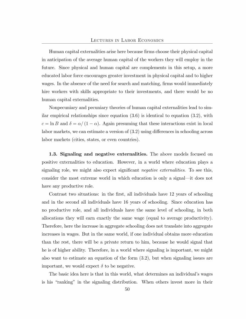
1.3. Signaling and negative externalities. The above models focused on

positive externalities to education. However, in a world where education plays a

signaling role, we might also expect significant negative externalities. To see this,

consider the most extreme world in which education is only a signal–it does not

have any productive role.

Contrast two situations: in the first, all individuals have 12 years of schooling

and in the second all individuals have 16 years of schooling. Since education has

no productive role, and all individuals have the same level of schooling, in both

allocations they will earn exactly the same wage (equal to average productivity).

Therefore, here the increase in aggregate schooling does not translate into aggregate

increases in wages. But in the same world, if one individual obtains more education

than the rest, there will be a private return to him, because he would signal that

he is of higher ability. Therefore, in a world where signaling is important, we might

also want to estimate an equation of the form (3.2), but when signaling issues are

important, we would expect δ to be negative.

The basic idea here is that in this world, what determines an individual’s wages

is his “ranking” in the signaling distribution. When others invest more in their

50


education, a given individual’s rank in the distribution declines, hence others are

creating a negative externality on this individual via their human capital investment.

2. Evidence

Ordinary Least Squares (OLS) estimation of equations like (3.2) using city or

state-level data yield very significant and positive estimates of δ, indicating substan-

tial positive human capital externalities. The leading example is the paper by Jim

Rauch.

There are at least two problems with this type OLS estimates. First, it may

be precisely high-wage cities or states that either attract a large number of high

education workers or give strong support to education. Rauch’s estimates were

using a cross-section of cities. Including city or state fixed affects ameliorates this

problem, but does not solve it, since states’ attitudes towards education and the

demand for labor may comove. The ideal approach would be to find a source of quasi-

exogenous variation in average schooling across labor markets (variation unlikely to

be correlated with other sources of variation in the demand for labor in the state).

Acemoglu and Angrist try to accomplish this using differences in compulsory

schooling laws. The advantage is that these laws not only affect individual schooling

but average schooling in a given area.

There is an additional econometric problem in estimating externalities, which

remains even if we have an instrument for average schooling in the aggregate. This

is that if individual schooling is measured with error (or for some other reason OLS

returns to individual schooling are not the causal effect), some of this discrepancy

between the OLS returns and the causal return may load on average schooling,

even when average schooling is instrumented. This suggests that we may need to

instrument for individual schooling as well (so as to get to the correct return to

individual schooling).

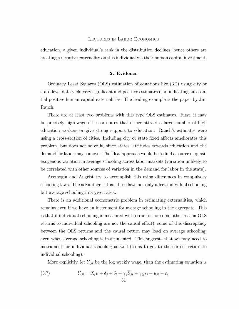
More explicitly, let Yijt be the log weekly wage, than the estimating equation is

(3.7) Yijt = X 0iμ+ δj + δt + γ1Sjt + γ2isi + ujt + εi,

51


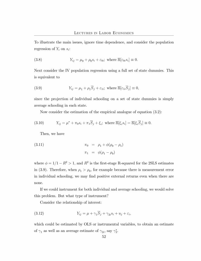
To illustrate the main issues, ignore time dependence, and consider the population

regression of Yi on si:

(3.8) Yij = μ0 + ρ0si + ε0i; where E[ε0isi] ≡ 0.

Next consider the IV population regression using a full set of state dummies. This

is equivalent to

(3.9) Yij = μ1 + ρ1Sj + ε1i; where E[ε1iSj] ≡ 0,

since the projection of individual schooling on a set of state dummies is simply

average schooling in each state.

Now consider the estimation of the empirical analogue of equation (3.2):

(3.10) Yij = μ∗ + π0si + π1Sj + ξi; where E[ξisi] = E[ξiSj] ≡ 0.

Then, we have

π0 = ρ1 + φ(ρ0 − ρ1)(3.11)

π1 = φ(ρ1 − ρ0)

where φ = 1/1−R2 > 1, and R2 is the first-stage R-squared for the 2SLS estimates

in (3.9). Therefore, when ρ1 > ρ0, for example because there is measurement error

in individual schooling, we may find positive external returns even when there are

none.

If we could instrument for both individual and average schooling, we would solve

this problem. But what type of instrument?

Consider the relationship of interest:

(3.12) Yij = μ+ γ1Sj + γ2isi + uj + εi,

which could be estimated by OLS or instrumental variables, to obtain an estimate

of γ1 as well as an average estimate of γ2i, say γ∗2.

52


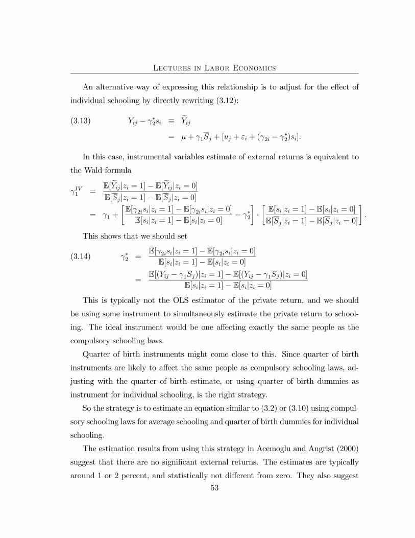
An alternative way of expressing this relationship is to adjust for the effect of

individual schooling by directly rewriting (3.12):

Yij − γ∗2si ≡ eYij(3.13)

= μ+ γ1Sj + [uj + εi + (γ2i − γ∗2)si].

In this case, instrumental variables estimate of external returns is equivalent to

the Wald formula

γIV1 =E[eYij|zi = 1]− E[eYij|zi = 0]E[Sj|zi = 1]− E[Sj|zi = 0]

= γ1 +

∙E[γ2isi|zi = 1]− E[γ2isi|zi = 0]E[si|zi = 1]− E[si|zi = 0]

− γ∗2

¸·∙E[si|zi = 1]− E[si|zi = 0]E[Sj|zi = 1]− E[Sj|zi = 0]

¸.

This shows that we should set

γ∗2 =E[γ2isi|zi = 1]− E[γ2isi|zi = 0]E[si|zi = 1]− E[si|zi = 0]

(3.14)

=E[(Yij − γ1Sj)|zi = 1]− E[(Yij − γ1Sj)|zi = 0]

E[si|zi = 1]− E[si|zi = 0]

This is typically not the OLS estimator of the private return, and we should

be using some instrument to simultaneously estimate the private return to school-

ing. The ideal instrument would be one affecting exactly the same people as the

compulsory schooling laws.

Quarter of birth instruments might come close to this. Since quarter of birth

instruments are likely to affect the same people as compulsory schooling laws, ad-

justing with the quarter of birth estimate, or using quarter of birth dummies as

instrument for individual schooling, is the right strategy.

So the strategy is to estimate an equation similar to (3.2) or (3.10) using compul-

sory schooling laws for average schooling and quarter of birth dummies for individual

schooling.

The estimation results from using this strategy in Acemoglu and Angrist (2000)

suggest that there are no significant external returns. The estimates are typically

around 1 or 2 percent, and statistically not different from zero. They also suggest

53


that in the aggregate signaling considerations are unlikely to be very important (at

the very least, they do not dominate positive externalities).

3. School Quality

Differences in school quality could be a crucial factor in differences in human

capital. Two individuals with the same years of schooling might have very different

skills and very different earnings because one went to a much better school, with

better teachers, instruction and resources. Differences in school quality would add

to the unobserved component of human capital.

A natural conjecture is that school quality as measured by teacher-pupil ratios,

spending per-pupil, length of school year, and educational qualifications of teachers

would be a major determinant of human capital. If school quality matters indeed a

lot, an effective way of increasing human capital might be to increase the quality of

instruction in schools.

This view was however challenged by a number of economists, most notably,

Hanushek. Hanushek noted that the substantial increase in spending per student

and teacher-pupil ratios, as well as the increase in the qualifications of teachers,

was not associated with improved student outcomes, but on the contrary with a

deterioration in many measures of high school students’ performance. In addition,

Hanushek conducted a meta-analysis of the large number of papers in the education

literature, and concluded that there was no overwhelming case for a strong effect of

resources and class size on student outcomes.

Although this research has received substantial attention, a number of careful

papers show that exogenous variation in class size and other resources are in fact

associated with sizable improvements in student outcomes.

Most notable:

(1) Krueger analyzes the data from the Tennessee Star experiment where stu-

dents were randomly allocated to classes of different sizes.

54


(2) Angrist and Lavy analyze the effect of class size on test scores using a unique

characteristic of Israeli schools which caps class size at 40, thus creating a

natural regression discontinuity as a function of the total number of students

in the school.

(3) Card and Krueger look at the effects of pupil-teacher ratio, term length

and relative teacher wage by comparing the earnings of individuals working

in the same state but educated in different states with different school

resources.

(4) Another paper by Card and Krueger looks at the effect of the “exogenously”

forced narrowing of the resource gap between black and white schools in

South Carolina on the gap between black and white pupils’ education and

subsequent earnings.

All of these papers find sizable effects of school quality on student outcomes.

Moreover, a recent paper by Krueger shows that there were many questionable

decisions in the meta-analysis by Hanushek, shedding doubt on the usefulness of

this analysis. On the basis of these various pieces of evidence, it is safe to conclude

that school quality appears to matter for human capital.

4. Peer Group Effects

Issues of school quality are also intimately linked to those of externalities. An

important type of externality, different from the external returns to education dis-

cussed above, arises in the context of education is peer group effects, or generally

social effects in the process of education. The fact that children growing up in

different areas may choose different role models will lead to this type of externali-

ties/peer group effects. More simply, to the extent that schooling and learning are

group activities, there could be this type of peer group effects.

There are a number of theoretical issues that need to be clarified, as well as

important work that needs to be done in understanding where peer group effects

are coming from. Moreover, empirical investigation of peer group effects is at its

55


infancy, and there are very difficult issues involved in estimation and interpretation.

Since there is little research in understanding the nature of peer group effects, here

we will simply take peer group effects as given, and briefly discuss some of its

efficiency implications, especially for community structure and school quality, and

then very briefly mention some work on estimating peer group affects.

4.1. Implications of peer group effects for mixing and segregation. An

important question is whether the presence of peer group effects has any particular

implications for the organization of schools, and in particular, whether children who

provide positive externalities on other children should be put together in a separate

school or classroom.

The basic issue here is equivalent to an assignment problem. The general princi-

ple in assignment problems, such as Becker’s famous model of marriage, is that if in-

puts from the two parties are complementary, there should be assortative matching,

that is the highest quality individuals should be matched together. In the context

of schooling, this implies that children with better characteristics, who are likely to

create more positive externalities and be better role models, should be segregated in

their own schools, and children with worse characteristics, who will tend to create

negative externalities will, should go to separate schools. This practically means

segregation along income lines, since often children with “better characteristics” are

those from better parental backgrounds, while children with worse characteristics

are often from lower socioeconomic backgrounds

So much is well-known and well understood. The problem is that there is an

important confusion in the literature, which involves deducing complementarity from

the fact that in equilibrium we do observe segregation (e.g., rich parents sending

their children to private schools with other children from rich parents, or living

in suburbs and sending their children to suburban schools, while poor parents live

in ghettos and children from disadvantaged backgrounds go to school with other

disadvantaged children in inner cities). This reasoning is often used in discussions

of Tiebout competition, together with the argument that allowing parents with

56


different characteristics/tastes to sort into different neighborhoods will often be

efficient.

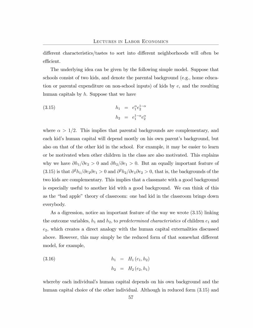
The underlying idea can be given by the following simple model. Suppose that

schools consist of two kids, and denote the parental background (e.g., home educa-

tion or parental expenditure on non-school inputs) of kids by e, and the resulting

human capitals by h. Suppose that we have

h1 = eα1 e1−α2(3.15)

h2 = e1−α1 eα2

where α > 1/2. This implies that parental backgrounds are complementary, and

each kid’s human capital will depend mostly on his own parent’s background, but

also on that of the other kid in the school. For example, it may be easier to learn

or be motivated when other children in the class are also motivated. This explains

why we have ∂h1/∂e2 > 0 and ∂h2/∂e1 > 0. But an equally important feature of

(3.15) is that ∂2h1/∂e2∂e1 > 0 and ∂2h2/∂e1∂e2 > 0, that is, the backgrounds of the

two kids are complementary. This implies that a classmate with a good background

is especially useful to another kid with a good background. We can think of this

as the “bad apple” theory of classroom: one bad kid in the classroom brings down

everybody.

As a digression, notice an important feature of the way we wrote (3.15) linking

the outcome variables, h1 and h2, to predetermined characteristics of children e1 and

e2, which creates a direct analogy with the human capital externalities discussed

above. However, this may simply be the reduced form of that somewhat different

model, for example,

h1 = H1 (e1, h2)(3.16)

h2 = H2 (e2, h1)

whereby each individual’s human capital depends on his own background and the

human capital choice of the other individual. Although in reduced form (3.15) and

57


(3.16) are very similar, they provide different interpretations of peer group effects,

and econometrically they pose different challenges, which we will discuss below.

The complementarity has two implications:

(1) It is socially efficient, in the sense of maximizing the sum of human capitals,

to have parents with good backgrounds to send their children to school with

other parents with good backgrounds. This follows simply from the defin-

ition of complementarity, positive cross-partial derivative, which is clearly

verified by the production functions in (3.15).

(2) It will also be an equilibrium outcome that parents will do so. To see this,

suppose that we have a situation in which there are two sets of parents

with background el and eh > el. Suppose that there is mixing. Now the

marginal willingness to pay of a parent with the high background to be in

the same school with the child of another high-background parent, rather

than a low-background student, is

eh − eαhe1−αl ,

while the marginal willingness to pay of a low background parent to stay

in the school with the high background parents is

eαl e1−αh − el.

The complementarity between eh and el in (3.15) implies that eh−eαhe1−αl >

eαl e1−αh − el.

Therefore, the high-background parent can always outbid the low-background

parent for the privilege of sending his children to school with other high-

background parents. Thus with profit maximizing schools, segregation will

arise as the outcome.

Next consider a production function with substitutability (negative cross-partial

derivative). For example,

h1 = φe1 + e2 − λe1/21 e

1/22(3.17)

h2 = e1 + φe2 − λe1/21 e

1/22

58


where φ > 1 and λ > 0 but small, so that human capital is increasing in parental

background. With this production function, we again have ∂h1/∂e2 > 0 and

∂h2/∂e1 > 0, but now in contrast to (3.15), we now have

∂2h1∂e2∂e1

and∂2h2∂e1∂e2

< 0.

This can be thought as corresponding to the “good apple” theory of the classroom,

where the kids with the best characteristics and attitudes bring the rest of the class

up.

In this case, because the cross-partial derivative is negative, the marginal will-

ingness to pay of low-background parents to have their kid together with high-

background parents is higher than that of high-background parents. With perfect

markets, we will observe mixing, and in equilibrium schools will consist of a mixture

of children from high- and low-background parents.

Now combining the outcomes of these two models, many people jump to the

conclusion that since we do observe segregation of schooling in practice, parental

backgrounds must be complementary, so segregation is in fact efficient. Again the

conclusion is that allowing Tiebout competition and parental sorting will most likely

achieve efficient outcomes.

However, this conclusion is not correct, since even if the correct production func-

tion was (3.17), segregation would arise in the presence of credit market problems.

In particular, the way that mixing is supposed to occur with (3.17) is that low-

background parents make a payment to high-background parents so that the latter

send their children to a mixed school. To see why such payments are necessary,

recall that even with (3.17) we have that the first derivatives are positive, that is

∂h1∂e2

> 0 and∂h2∂e1

> 0.

This means that everything else being equal all children benefit from being in the

same class with other children with good backgrounds. With (3.17), however, chil-

dren from better backgrounds benefit less than children from less good backgrounds.

59


This implies that there has to be payments from parents of less good backgrounds

to high-background parents.

Such payments are both difficult to implement in practice, and practically im-

possible taking into account the credit market problems facing parents from poor

socioeconomic status.

This implies that, if the true production function is (3.17) but there are credit

market problems, we will observe segregation in equilibrium, and the segregation

will be inefficient. Therefore we cannot simply appeal to Tiebout competition, or

deduce efficiency from the equilibrium patterns of sorting.

Another implication of this analysis is that in the absence of credit market

problems (and with complete markets), cross-partials determine the allocation of

students to schools. With credit market problems, first there of it has become

important. This is a general result, with a range of implications for empirical work.

4.2. The Benabou model. A similar point is developed by Benabou even

in the absence of credit market problems, but relying on other missing markets.

His model has competitive labor markets, and local externalities (externalities in

schooling in the local area). All agents are assumed to be ex ante homogeneous,

and will ultimately end up either low skill or high skill.

Utility of agent i is assumed to be

U i = wi − ci − ri

where w is the wage, c is the cost of education, which is necessary to become both

low skill or high skill, and r is rent.

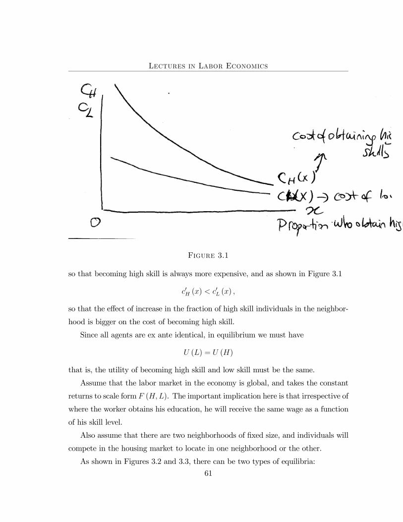
The cost of education is assumed to depend on the fraction of the agents in the

neighborhood, denoted by x, who become high skill. In particular, we have cH (x)

and cL (x) as the costs of becoming high skill and low skill. Both costs are decreasing

in x, meaning that when there are more individuals acquiring high skill, becoming

high skill is cheaper (positive peer group effects). In addition, we have

cH (x) > cL (x)

60


Figure 3.1

so that becoming high skill is always more expensive, and as shown in Figure 3.1

c0H (x) < c0L (x) ,

so that the effect of increase in the fraction of high skill individuals in the neighbor-

hood is bigger on the cost of becoming high skill.

Since all agents are ex ante identical, in equilibrium we must have

U (L) = U (H)

that is, the utility of becoming high skill and low skill must be the same.

Assume that the labor market in the economy is global, and takes the constant

returns to scale form F (H,L). The important implication here is that irrespective of

where the worker obtains his education, he will receive the same wage as a function

of his skill level.

Also assume that there are two neighborhoods of fixed size, and individuals will

compete in the housing market to locate in one neighborhood or the other.

As shown in Figures 3.2 and 3.3, there can be two types of equilibria:

61


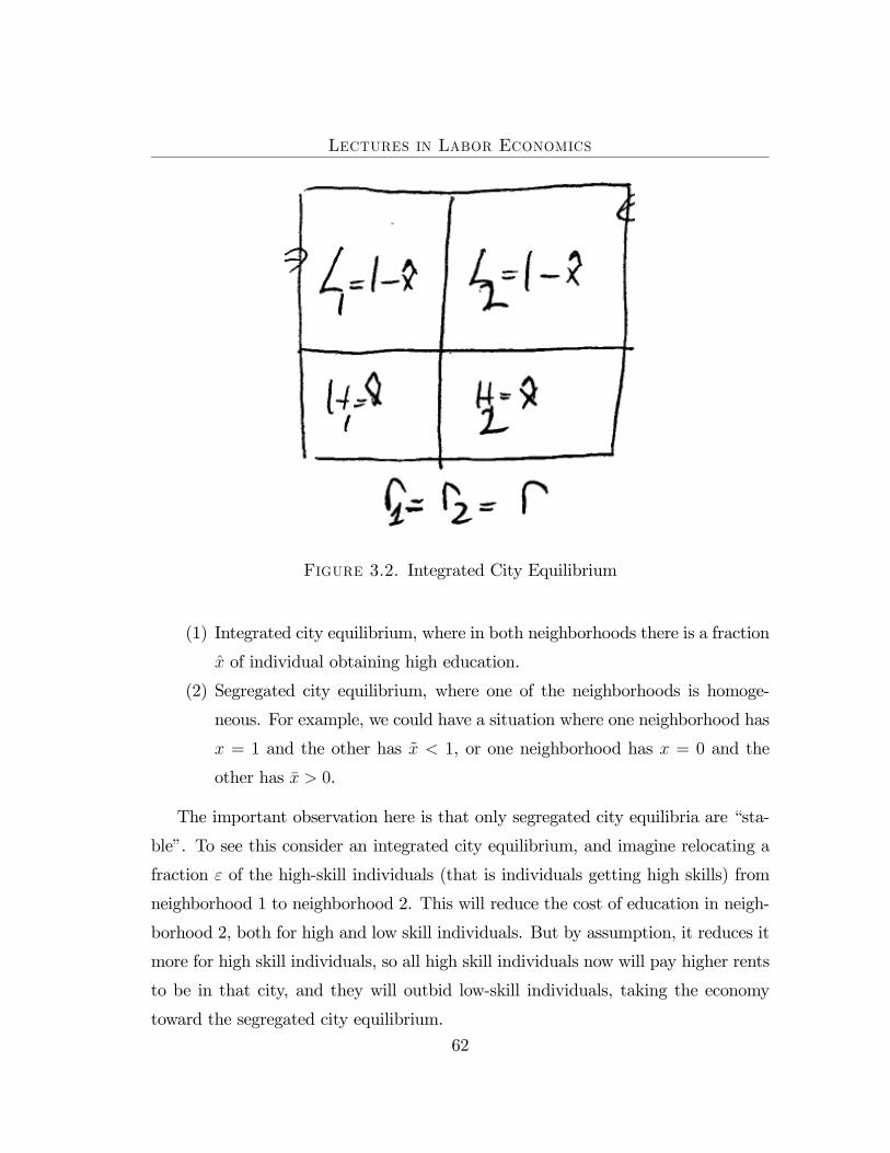
Figure 3.2. Integrated City Equilibrium

(1) Integrated city equilibrium, where in both neighborhoods there is a fraction

x of individual obtaining high education.

(2) Segregated city equilibrium, where one of the neighborhoods is homoge-

neous. For example, we could have a situation where one neighborhood has

x = 1 and the other has x < 1, or one neighborhood has x = 0 and the

other has x > 0.

The important observation here is that only segregated city equilibria are “sta-

ble”. To see this consider an integrated city equilibrium, and imagine relocating a

fraction ε of the high-skill individuals (that is individuals getting high skills) from

neighborhood 1 to neighborhood 2. This will reduce the cost of education in neigh-

borhood 2, both for high and low skill individuals. But by assumption, it reduces it

more for high skill individuals, so all high skill individuals now will pay higher rents

to be in that city, and they will outbid low-skill individuals, taking the economy

toward the segregated city equilibrium.

62


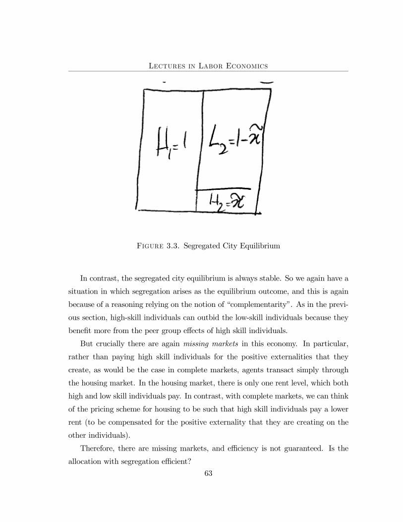
Figure 3.3. Segregated City Equilibrium

In contrast, the segregated city equilibrium is always stable. So we again have a

situation in which segregation arises as the equilibrium outcome, and this is again

because of a reasoning relying on the notion of “complementarity”. As in the previ-

ous section, high-skill individuals can outbid the low-skill individuals because they

benefit more from the peer group effects of high skill individuals.

But crucially there are again missing markets in this economy. In particular,

rather than paying high skill individuals for the positive externalities that they

create, as would be the case in complete markets, agents transact simply through

the housing market. In the housing market, there is only one rent level, which both

high and low skill individuals pay. In contrast, with complete markets, we can think

of the pricing scheme for housing to be such that high skill individuals pay a lower

rent (to be compensated for the positive externality that they are creating on the

other individuals).

Therefore, there are missing markets, and efficiency is not guaranteed. Is the

allocation with segregation efficient?

63


It turns out that it may or may not. To see this consider the problem of a utili-

tarian social planner maximizing total output minus costs of education for workers.

This implies that the social planner will maximize

F (H,L)−H1cH (x1)−H2cH (x2)− L1cL (x1)− L2cL (x2)

where

x1 =H1

L1 +H1and x2 =

H2

L2 +H2

This problem can be broken into two parts: first, the planner will choose the ag-

gregate amount of skilled individuals, and then she will choose how to actually

allocate them between the two neighborhoods. The second part is simply one of

cost minimization, and the solution depends on whether

Φ (x) = xcH (x) + (1− x) cL (x)

is concave or convex. This function is simply the cost of giving high skills to a

fraction x of the population. When it is convex, it means that it is best to choose

the same level of x in both neighborhoods, and when it is concave, the social planner

minimizes costs by choosing two extreme values of x in the two neighborhoods.

It turns out that this function can be convex, i.e. Φ00 (x) > 0. More specifically,

we have:

Φ00 (x) = 2 (c0H (x)− c0L (x)) + x (c00H (x)− c00L (x)) + c00L (x)

We can have Φ00 (x) > 0 when the second and third terms are large. Intuitively,

this can happen because although a high skill individual benefits more from being

together with other high skill individuals, he is also creating a positive externality on

low skill individuals when he mixes with them. This externality is not internalized,

potentially leading to inefficiency.

This model gives another example of why equilibrium segregation does not imply

efficient segregation.

4.3. Empirical issues and evidence. Peer group effects are generally difficult

to identify. In addition, we can think of two alternative formulations where one is

practically impossible to identify satisfactorily. To discuss these issues, let us go back

64


to the previous discussion, and recall that the two “structural” formulations, (3.15)

and (3.16), have very similar reduced forms, but the peer group effects work quite

differently, and have different interpretations. In (3.15), it is the (predetermined)

characteristics of my peers that determine my outcomes, whereas in (3.16), it is the

outcomes of my peers that matter. Above we saw how to identify externalities in

human capital, which is in essence similar to the structural form in (3.15). More

explicitly, the equation of interest is

(3.18) yij = θxij + αXj + εij

where X is average characteristic (e.g., average schooling) and yij is the outcome

of the ith individual in group j. Here, for identification all we need is exogenous

variation in X.

The alternative is

(3.19) yij = θxij + αYj + εij

where Y is the average of the outcomes. Some reflection will reveal why the parame-

ter α is now practically impossible to identify. Since Yj does not vary by individual,

this regression amounts to one of Yj on itself at the group level. This is a serious

econometric problem. One imperfect way to solve this problem is to replace Yj on

the right hand side by Y −ij which is the average excluding individual i. Another

approach is to impose some timing structure. For example:

yijt = θxijt + αYj,t−1 + εijt

There are still some serious problems irrespective of the approach taken. First, the

timing structure is arbitrary, and second, there is no way of distinguishing peer

group effects from “common shocks”.

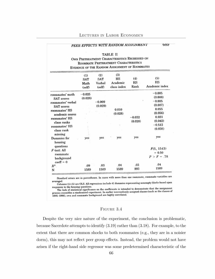
As an example consider the paper by Sacerdote, which uses random assignment of

roommates in Dartmouth. He finds that the GPAs of randomly assigned roommates

are correlated, and interprets this as evidence for peer group effects. The next table

summarizessome of the key results.

65


Figure 3.4

Despite the very nice nature of the experiment, the conclusion is problematic,

because Sacerdote attempts to identify (3.19) rather than (3.18). For example, to the

extent that there are common shocks to both roommates (e.g., they are in a noisier

dorm), this may not reflect peer group effects. Instead, the problem would not have

arisen if the right-hand side regressor was some predetermined characteristic of the

66


roommate (i.e., then we would be estimating something similar to (3.18) rather than

(3.19)).

67

Documents

CHAPTER 2econ.lse.ac.uk/staff/spischke/ec533/Acemoglu Autor chapter 2.pdf · CHAPTER 2 Human Capital and Signaling 1. The Basic Model of Labor Market Signaling The models we have