Chapter 20Large Eddy Simulation of Wind FarmAerodynamics with Energy-Conserving Schemes

Dhruv Mehta

Abstract In order to truly realise the potential of wind power, it is vital tounderstand the aerodynamic losses over a wind farm. The current chapter highlightsthe importance of aerodynamic analysis of offshore wind farms, and presents asummarized review of Large Eddy Simulation literature. Furthermore, the chapterpresents the objectives of the current research and concludes with a case study.

20.1 Introduction

This chapter presents a study on the Large Eddy Simulation of wind farm aerody-namics. Wind farm aerodynamics (WFA) deals with the interaction between windturbine wakes and the atmospheric boundary layer (ABL), as they develop acrossthe length of the wind farm. At times, the wakes also interact with each other andwith other wind turbines (Mehta et al. 2014).

The study of WFA is crucial as it provides insight into the air flow through awind farm, which eventually provides the energy that is converted into electricityby wind turbines. Therefore, one can assess the power produced by a wind farm byaerodynamically analysing the flow through the farm. The study of WFA requiresaerodynamic data, which is generally gathered through meteorological masts inexisting wind farms.

With the apparatus placed on these masts, we can measure the velocity andturbulence intensity (TI)—albeit at only a single point. In case the apparatus is anarray of instruments, one may be able to measure the velocity (and TI) at morethan a single point. Nonetheless, even in the best cases, the aerodynamic data fora few points on a wind farm is not enough to assess the power produced by thewind farm. Further, the erratic nature of the atmosphere makes it hard to relate themeasured velocity (or TI) to its cause. For example, one cannot be certain whether

D. Mehta (�)Wind Energy Research Institute (DUWIND), Delft University, Kluyverweg 1, 2629 HS Delft,Netherlands

Energy Research Centre of the Netherlands (ECN), Westerduinweg 3, 1755 LE Petten,Netherlandse-mail: d.mehta@tudelft.nl

© The Author(s) 2016W. Ostachowicz et al. (eds.), MARE-WINT, DOI 10.1007/978-3-319-39095-6_20

347

348 D. Mehta

the measured velocity (or TI) is from a single turbine’s wake, or due to a sudden gustthrough the farm etc. Thus, for a complete insight, it is important to complementexperimental data with numerical data from simulations.

20.2 Simulation

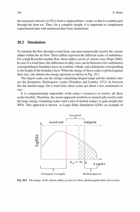
To simulate the flow through a wind farm, one must numerically resolve the variouseddies within the air flow. These eddies represent the different scales of turbulence.For a high Reynolds number flow, these eddies can be of various sizes (Pope 2000).In case of a wind farm, this difference in eddy sizes can be between a few millimetrescorresponding to boundary layer on a turbine’s blade, and a kilometre correspondingto the height of the boundary layer. When the energy of these scales is plotted againsttheir size, one obtains the energy spectrum as shown in Fig. 20.1.

The largest scales are the energy-containing integral range and the smallest onesare the dissipative, Kolmogorov scales (Tennekes and Lumley 1972). In betweenlies the inertial range. On a wind farm, these scales are about a few centimetres insize.

It is computationally impossible (with today’s resources) to resolve all thesescales feasibly. Therefore, the wisest approach would be to numerically resolve onlythe large energy containing scales (and a part of inertial range), to gain insight intoWFA. This approach is known as Large Eddy Simulation (LES); an example of

Fig. 20.1 The energy of the various eddies (y-axis) in a flow, plotted against their size (x-axis)

20 Large Eddy Simulation of Wind Farm Aerodynamics with Energy-. . . 349

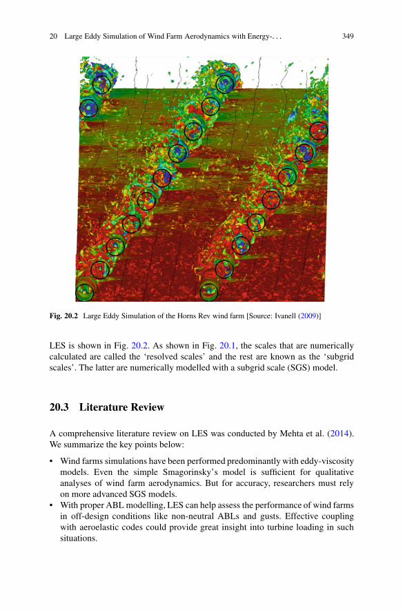
Fig. 20.2 Large Eddy Simulation of the Horns Rev wind farm [Source: Ivanell (2009)]

LES is shown in Fig. 20.2. As shown in Fig. 20.1, the scales that are numericallycalculated are called the ‘resolved scales’ and the rest are known as the ‘subgridscales’. The latter are numerically modelled with a subgrid scale (SGS) model.

20.3 Literature Review

A comprehensive literature review on LES was conducted by Mehta et al. (2014).We summarize the key points below:

• Wind farms simulations have been performed predominantly with eddy-viscositymodels. Even the simple Smagorinsky’s model is sufficient for qualitativeanalyses of wind farm aerodynamics. But for accuracy, researchers must relyon more advanced SGS models.

• With proper ABL modelling, LES can help assess the performance of wind farmsin off-design conditions like non-neutral ABLs and gusts. Effective couplingwith aeroelastic codes could provide great insight into turbine loading in suchsituations.

350 D. Mehta

• Wind farm simulations rely on accurate wake-ABL interaction, which is possibleonly with a correct ABL model. This is of great consequence for simulating largewind farms on which the ABL evolves into a wind turbine-ABL. Generating asynthetic ABL requires lesser computational effort than precursor simulationswith LES, but lacks the statistical correlations that exist in a physical ABL.

• Using the Scale Dependent Dynamic model with Lagrangian averaging generatesan ABL that is accurate enough for wind farm simulations, but is computationallyexpensive. Nonetheless, it retains its precision even on coarse grids making itsuitable for LES.

• From simulations of the Horns Rev wind farm, it is apparent that the performanceof engineering models is comparable to that of certain LES codes, as far asgenerating averaged statistics. When done with accurate ABL modelling and withadvanced SGS models, on relatively refined grids, LES delivers a substantiallybetter performance.

• LES data can be utilised to enhance simple engineering models to retaincomputational efficiency but ensuring better accuracy.

• Numerical schemes for LES must ensure zero numerical dissipation for highaccuracy. Pseudo-spectral and Energy-Conserving spatial discretisation schemesare useful in this regard; the latter however requires a higher-order formulationto be as accurate as the former. Additionally, energy-conserving time integrationwith zero dissipation would help speed up computations, but requires furthermodifications to avert loss in accuracy and stability.

• A stress-free upper boundary is most appropriate for wind farm simulations.Periodic boundaries required by spectral schemes can be avoided with Energy-Conserving schemes, which are however not as accurate as the former.

• SGS models have been compared in terms of their ability to simulate the ABL.It is clear that above beyond a certain resolution, the effect of the SGS model onABL is nullified and even a simple model is sufficient for an ABL simulation.However, such a conclusion with regard to wind farm simulations is yet to bedrawn.

Concerning LES, it is certain that no SGS model is complete and their efficacyis situation-dependent. Smagorinsky’s model and its derivatives are popular asthey are easily implementable and capable of producing good data on wind farmaerodynamics, despite their assumptions lacking conclusive evidence. Regardingcoarse grids, it would be wise to develop numerical schemes instead of relyingon excess computational power. LES codes cannot count on upwind schemes ofstability because the numerical dissipation will dampen the resolved scales, moreso on coarse grids. High-order spectral methods are thus common in LES butare computationally expensive. On the other hand, Energy-conserving schemes arefree from numerical dissipation and permit the use of non-periodic boundaries, butrequire further investigation at this stage.

20 Large Eddy Simulation of Wind Farm Aerodynamics with Energy-. . . 351

In terms of boundary conditions, Monin-Obukov’s (Panofsky and Dutton 1984)approach remains the only option for modelling the ABL, despite being deemedunsuitable for LES. Lately, research has been focussed on developing a moreappropriate technique that could be adapted for inhomogeneous terrains, butexperiments would be more instrumental in enhancing the existing approach.

20.4 Power Losses and Observations

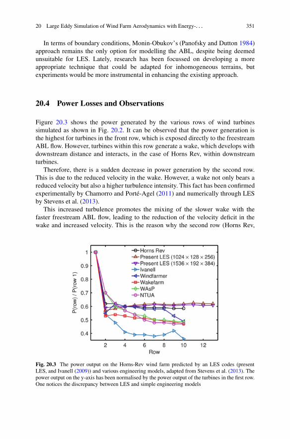
Figure 20.3 shows the power generated by the various rows of wind turbinessimulated as shown in Fig. 20.2. It can be observed that the power generation isthe highest for turbines in the front row, which is exposed directly to the freestreamABL flow. However, turbines within this row generate a wake, which develops withdownstream distance and interacts, in the case of Horns Rev, within downstreamturbines.

Therefore, there is a sudden decrease in power generation by the second row.This is due to the reduced velocity in the wake. However, a wake not only bears areduced velocity but also a higher turbulence intensity. This fact has been confirmedexperimentally by Chamorro and Porté-Agel (2011) and numerically through LESby Stevens et al. (2013).

This increased turbulence promotes the mixing of the slower wake with thefaster freestream ABL flow, leading to the reduction of the velocity deficit in thewake and increased velocity. This is the reason why the second row (Horns Rev,

Fig. 20.3 The power output on the Horns-Rev wind farm predicted by an LES codes (presentLES, and Ivanell (2009)) and various engineering models, adapted from Stevens et al. (2013). Thepower output on the y-axis has been normalised by the power output of the turbines in the first row.One notices the discrepancy between LES and simple engineering models

352 D. Mehta

black line in Fig. 20.3), generates the highest power amongst all downstream rows.Further, the increased turbulence reaches a peak value after the wake from the firstturbine interacts with the second turbine, leading to a slower wake; thus, after onewake-turbine interaction. At times, this could happen after two such wake-turbineinteractions, in case the inflow turbulence is low (Mehta et al. 2014).

Once, the wake generated turbulence reaches its peak value, the recovery of thereduced velocity in the wake also reaches its limit. Therefore, after one or twowake-turbine interactions, the wake does not recover much, as a result, one noticesa decline in power production across the rows on a wind farm. Nevertheless, thedecrease is not steep as compared to the one noticed within the first two rows. Thefact that the added turbulence has reached a steady peak value, ensures that the wakerecovers after every wake-turbine interaction, to a value that is more or less similarto the inflow value. In effect, beyond the second or third row, the horizontal flow isfully developed, leading a similar power prediction as seen in Fig. 20.3 (Calaf et al.2010).

Figure 20.3 also compares the date from LES and engineering models. Thesemodels are very simple and built upon the simplification of the flow phenomena. Asa result, these models are fast and computationally efficient but not very accurate.Further, their accuracy is mostly related to the prediction of the average poweroutput over a range of wind directions, and not for a particular inflow direction,which requires the application of LES (Barthelmie et al. 2009).

20.5 Research Objectives

The current research involves three phases:

• Implementing an SGS model in the Energy-Conserving Navier-Stokes (ECNS)code.

• Analysing energy-conserving (EC) spatial discretisation and EC time integrationin terms of accuracy and efficiency.

• Validating the combination of the ECNS and the chosen SGS model for windfarm simulations.

20.6 Tests and Results

The following are the tests conducted, the results obtained and the conclusionsdrawn.

20 Large Eddy Simulation of Wind Farm Aerodynamics with Energy-. . . 353

20.6.1 EC Time Integration

EC time integration available within the ECNS code is unconditionally stable forany time step. Further, it introduces no numerical dissipation during the simulation(Sanderse 2013). However, according to the literature, most existing LES codeswould rely on non-EC time integration.

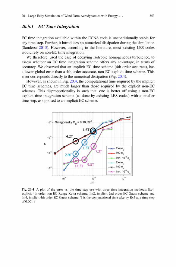
We therefore, used the case of decaying isotropic homogeneous turbulence, toassess whether an EC time integration scheme offers any advantage, in terms ofaccuracy. We observed that an implicit EC time scheme (4th order accurate), hasa lower global error than a 4th order accurate, non-EC explicit time scheme. Thiserror corresponds directly to the numerical dissipation (Fig. 20.4).

However, as shown in Fig. 20.4, the computational time required by the implicitEC time schemes, are much larger than those required by the explicit non-ECschemes. This disproportionality is such that, one is better off using a non-ECexplicit time integration scheme (as done by existing LES codes) with a smallertime step, as opposed to an implicit EC scheme.

Fig. 20.4 A plot of the error vs. the time step use with three time integration methods: Ex4,explicit 4th order non-EC Runge-Kutta scheme; Im2, implicit 2nd order EC Gauss scheme andIm4, implicit 4th order EC Gauss scheme. T is the computational time take by Ex4 at a time stepof 0.001 s

354 D. Mehta

20.6.2 EC Spatial Discretisation

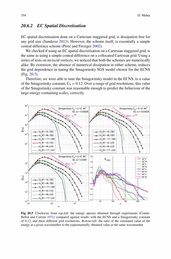
EC spatial discretisation done on a Cartesian staggered grid, is dissipation free forany grid size (Sanderse 2013). However, the scheme itself, is essentially a simplecentral difference scheme (Peric and Ferziger 2002).

We checked if using an EC spatial discretisation on a Cartesian staggered grid, isthe same as using a simple central difference on a collocated Cartesian grid. Using aseries of tests on inviscid vortices, we noticed that both the schemes are numericallyalike. By extension, the absence of numerical dissipation in either scheme, reducesthe grid dependence in tuning the Smagorinsky SGS model chosen for the ECNS(Fig. 20.5).

Therefore, we were able to tune the Smagorinsky model in the ECNS, to a valueof the Smagorinsky constant, CS D 0.12. Over a range of grid resolutions, this valueof the Smagorinsky constant was reasonable enough to predict the behaviour of thelarge energy-containing scales, correctly.

Fig. 20.5 Clockwise from top-left: the energy spectra obtained through experiments (Comté-Bellot and Corrsin 1971) compared against results with the ECNS and a Smagorisnky constantof 0.12, and three different grid resolutions. Bottom-left: the ratio of the simulated value of theenergy at a given wavenumber to the experimentally obtained value at the same wavenumber

20 Large Eddy Simulation of Wind Farm Aerodynamics with Energy-. . . 355

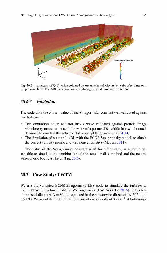
Fig. 20.6 Isosurfaces of Q-Criterion coloured by streamwise velocity in the wake of turbines on asimple wind farm. The ABL is neutral and runs through a wind farm with 15 turbines

20.6.3 Validation

The code with the chosen value of the Smagorinsky constant was validated againsttwo test-cases.

• The simulation of an actuator disk’s wave validated against particle imagevelocimetry measurements in the wake of a porous disc within in a wind tunnel,designed to emulate the actuator disk concept (Lignarolo et al. 2014).

• The simulation of a neutral-ABL with the ECNS-Smagorinsky model, to obtainthe correct velocity profile and turbulence statistics (Meyers 2011).

The value of the Smagorinsky constant is fit for either case; as a result, weare able to simulate the combination of the actuator disk method and the neutralatmospheric boundary layer (Fig. 20.6).

20.7 Case Study: EWTW

We use the validated ECNS-Smagorinsky LES code to simulate the turbines atthe ECN Wind Turbine Test-Site Wieringermeer (EWTW) (Bot 2015). It has fiveturbines of diameter DD 80 m, separated in the streamwise direction by 305 m or3.812D. We simulate the turbines with an inflow velocity of 8 m s�1 at hub-height

356 D. Mehta

240

200

160

120

80

40

00 2 4 6 8 2 4 6 8 2 4 6 8

T1T2T3T4T5T1,–1D

1D 2D 3D

u (m/s)

h (m

)

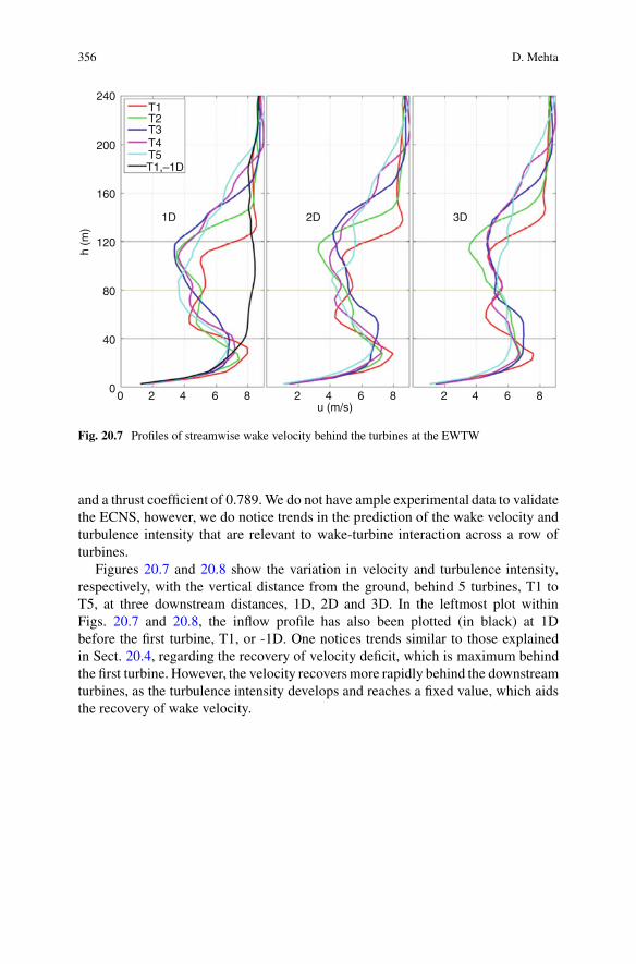
Fig. 20.7 Profiles of streamwise wake velocity behind the turbines at the EWTW

and a thrust coefficient of 0.789. We do not have ample experimental data to validatethe ECNS, however, we do notice trends in the prediction of the wake velocity andturbulence intensity that are relevant to wake-turbine interaction across a row ofturbines.

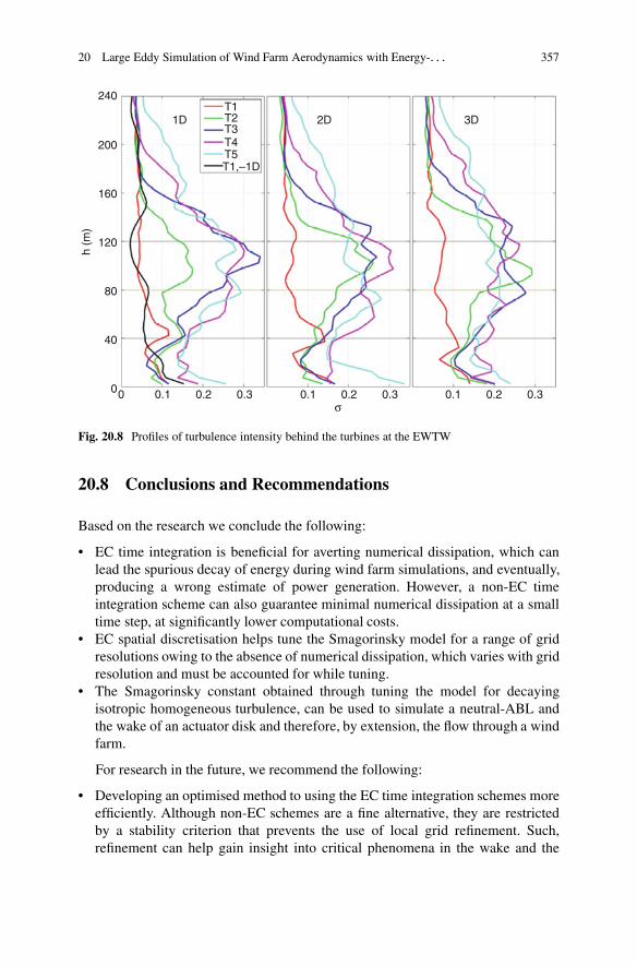
Figures 20.7 and 20.8 show the variation in velocity and turbulence intensity,respectively, with the vertical distance from the ground, behind 5 turbines, T1 toT5, at three downstream distances, 1D, 2D and 3D. In the leftmost plot withinFigs. 20.7 and 20.8, the inflow profile has also been plotted (in black) at 1Dbefore the first turbine, T1, or -1D. One notices trends similar to those explainedin Sect. 20.4, regarding the recovery of velocity deficit, which is maximum behindthe first turbine. However, the velocity recovers more rapidly behind the downstreamturbines, as the turbulence intensity develops and reaches a fixed value, which aidsthe recovery of wake velocity.

20 Large Eddy Simulation of Wind Farm Aerodynamics with Energy-. . . 357

240

200

160

120

80

40

00 0.1 0.2 0.3 0.1 0.2 0.3 0.1 0.2 0.3

h (m

)

T1T2T3T4T5T1,–1D

1D 2D 3D

σ

Fig. 20.8 Profiles of turbulence intensity behind the turbines at the EWTW

20.8 Conclusions and Recommendations

Based on the research we conclude the following:

• EC time integration is beneficial for averting numerical dissipation, which canlead the spurious decay of energy during wind farm simulations, and eventually,producing a wrong estimate of power generation. However, a non-EC timeintegration scheme can also guarantee minimal numerical dissipation at a smalltime step, at significantly lower computational costs.

• EC spatial discretisation helps tune the Smagorinsky model for a range of gridresolutions owing to the absence of numerical dissipation, which varies with gridresolution and must be accounted for while tuning.

• The Smagorinsky constant obtained through tuning the model for decayingisotropic homogeneous turbulence, can be used to simulate a neutral-ABL andthe wake of an actuator disk and therefore, by extension, the flow through a windfarm.

For research in the future, we recommend the following:

• Developing an optimised method to using the EC time integration schemes moreefficiently. Although non-EC schemes are a fine alternative, they are restrictedby a stability criterion that prevents the use of local grid refinement. Such,refinement can help gain insight into critical phenomena in the wake and the

358 D. Mehta

ABL as a whole. Using an EC time scheme that is implicit, will not only removethe restriction on grid refinement but also avert numerical dissipation.

• Simple schemes such as the central difference scheme in OpenFOAM can readilybe used for wind farm aerodynamics, instead of developing new computationalmethods.

Open Access This chapter is distributed under the terms of the Creative Commons Attribution-NonCommercial 4.0 International License (http://creativecommons.org/licenses/by-nc/4.0/),which permits any noncommercial use, duplication, adaptation, distribution and reproductionin any medium or format, as long as you give appropriate credit to the original author(s) and thesource, provide a link to the Creative Commons license and indicate if changes were made.

The images or other third party material in this chapter are included in the work’s CreativeCommons license, unless indicated otherwise in the credit line; if such material is not includedin the work’s Creative Commons license and the respective action is not permitted by statutoryregulation, users will need to obtain permission from the license holder to duplicate, adapt orreproduce the material.

References

Barthelmie RJ, Frandsen ST, Hansen K et al (2009) Modelling the impact of Wakes on PowerOutput at Nysted and Horns. Paper presented at the EWEC 2009, European wind energyconference and exhibition, Marseille 16–19 March 2009

Bot ETG (2015) FarmFlow validation against full scale wind farms, Technical Report ECN-E-15-045. In: Energy research Centre of the Netherlands publications. Available via ECN. https://www.ecn.nl/publications/PdfFetch.aspx?nr=ECN-E--15-045. Accessed 12 Apr 2016

Calaf M, Meneveau C, Meyers J (2010) Large Eddy Simulation study of fully developed wind-turbine array boundary layers. Phys Fluids. doi:10.1063/1.3291077

Chamorro LP, Porté-Agel F (2011) Turbulent flow inside and above a wind farm: a wind tunnelstudy. Energies 4:1916–1936

Comté-Bellot G, Corrsin S (1971) Simple Eulerian time correlation of full and narrow bandvelocity signals in grid generated isotropic turbulence. J Fluid Mech 48:272–337

Ivanell SSA (2009) Numerical computations of wind turbine wakes. In: Technical reports fromthe Royal Institute of Technology, Linné Flow Centre, Department of Mechanics, Stock-holm. Available via KTH. https://sverigesradio.se/diverse/appdata/isidor/files/3345/10845.pdf.Accessed 12 Apr 2016

Lignarolo L, Ragni D, Krishnaswami C et al (2014) Experimental analysis of a horizontal axiswind-turbine model. Renew Energ 70:31–46

Mehta D, van Zuijlen AH, Koren B et al (2014) LES of wind farm aerodynamics: a review. J WindEng Ind Aerod 133:1–17

Meyers J (2011) Error-landscape assessment of large-eddy simulations: a review of the methodol-ogy. J Sci Comput 49:65–77

Panofsky H, Dutton J (1984) Atmospheric turbulence: models and methods for engineeringapplications. Wiley, New York

Peric M, Ferziger J (2002) Computational methods for fluid dynamics. Springer, BerlinPope SB (2000) Turbulent flows. Cambridge University Press, CambridgeSanderse B (2013) Energy conserving discretisation methods for the incompressible Navier-

Stokes equations: application to the simulation of wind-turbine wakes. Dissertation, EindhovenUniversity of Technology

Stevens RJAM, Gayme DF, Meneveau C (2013) Effect of turbine alignment on the averagepower output of wind farm. In: Abstracts of the ICOWES 2013 international conference onaerodynamics of offshore wind energy systems and wakes, Lyngby, 17–19 June 2013

Tennekes H, Lumley JL (1972) A first course in turbulence. MIT Press, London