Embed Size (px)
Citation preview
Chapter 2Statics
2.1 A Concept of Equilibrium
If the velocity and acceleration of every particle in a material system are equal tozero, such a system is at rest. On the other hand, as we recall, from Newton’s firstlaw it follows that a particle having mass to which no force is applied or the appliedforces are balanced is either at rest or in uniform motion along a straight line.
If a material system acted on by a force system does not change its positionduring an arbitrarily (infinitely) long time, we say that it is in equilibrium under theaction of that force system.
Statics is the branch of mechanics that focuses on the equilibrium of materialbodies (particles) under the action of forces (moments of force). It deals with theanalysis of forces acting on material systems at rest or moving in uniform motionalong a straight line and, as will become clear later, may be treated as a specialcase of dynamics. This chapter, devoted to statics, might be extended by materialpresented in books devoted to classical mechanics like, for instance, [1–25].
It turns out that for a material system to remain in equilibrium under the actionof a certain force system, that force system must satisfy the so-called equilibriumconditions.
In order to emphasize the lack of time influence on equilibrium conditions, instatics the term state of static equilibrium is often used. In general, statics can bedivided into elementary statics and analytical statics. In the case of elementarystatics, during analysis of static equilibrium states vector algebra and graphicalmethods are applied. On the other hand, in the case of analytical statics the conceptsof virtual displacement and principle of virtual work are used, which in part wasdiscussed in Chap. 1.
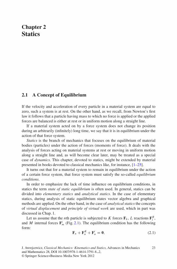
Let us assume that the nth particle is subjected to K forces Fk, L reactions FRl ,and M internal forces Fim (Fig. 2.1). The equilibrium condition has the followingform:
Fn C FRn C Fin D 0; (2.1)
J. Awrejcewicz, Classical Mechanics: Kinematics and Statics, Advances in Mechanicsand Mathematics 28, DOI 10.1007/978-1-4614-3791-8 2,© Springer Science+Business Media New York 2012
23
24 2 Statics
where
Fn DKX
kD1Fk; FRn D
LX
lD1FRl ; Fin D
MX
mD1Fim: (2.2)
After multiplying both sides of (2.1) by the unit vectors Ej of the coordinatesystem OX1X2X3 (scalar product) and taking into account (2.2), we obtain the so-called analytical conditions of equilibrium of the form
KX
kD1Fkxj C
LX
lD1F Rlxj
CMX
mD1F imxj
D 0; j D 1; 2; 3: (2.3)
Because in general the forces may be projected onto the axes of any curvilinearcoordinate system, the following theorem is valid.
Theorem 2.1. A particle is in equilibrium if the sum of projections of external,internal, and reaction forces (acting on this particle) onto axes of the adoptedcoordinate system is equal to zero.
The three conditions (2.3) are necessary, but not sufficient, for the particle toremain at rest, as follows from Newton’s first law.
In order to formulate the equilibrium conditions for a whole material systemor a body (infinite number of particles), one should formulate such equations forevery particle n 2 Œ1; N � (N D 1 in the case of the body) and add them together,obtaining
S DNX
nD1.Fn C FRn C Fin/ D 0; (2.4)
where N is the number of particles of the material system.A system of particles will be in equilibrium if the sum of projections of external,
internal, and reaction forces, acting on every particle of the system, onto three axesof the adopted coordinate system is equal to zero. After projection we obtain 3Nanalytical equilibrium conditions for the system of N particles.
According to Newton’s third law, the internal forces are the effect of action andreaction and they are pairs of opposite forces, which means that they cancel out oneanother, that is,
PNnD1 Fin D 0.
Observe that the result of action of a given force on a rigid body remainsunchanged when that force is applied at any point of its line of action (the so-calledprinciple of transmissibility), and hence the forces acting on a rigid body can berepresented by sliding vectors. In other words, if instead of a force F at a givenpoint of the rigid body we apply a force F0 of the same magnitude and direction ata point A0 .A ¤ A0/, then the equilibrium state, or motion of a rigid body, is notaffected provided that the two forces have the same line of action. The principle oftransmissibility is based on experimental evidence, and the mentioned forces F andF0 are called equivalent.
2.1 A Concept of Equilibrium 25
Fig. 2.1 A particle n (point A) under the action of forces Fk and reactions FRl , and the sameparticle under the action of the resultant forces F and reactions FR (internal forces not shown)
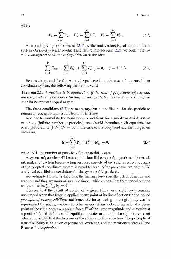
Fig. 2.2 Concurrent forces acting on a rigid body (a) and a force polygon (b)
In Fig. 2.1 it was shown that all forces are applied at a single point A. Now wewill consider a more general case of a rigid body loaded with a discrete system offorces applied at points An of magnitudes Fn; n D 1; : : : ; N and of lines of actionpassing through a certain point A (Fig. 2.2).
The force system that we call concurrent and those forces need not lie in acommon plane. Because, by assumption, the lines of action of the forces intersectat point A, the system in Fig. 2.2a is equivalent to the force system depicted inFig. 2.2b. Adding successively the force vectors and using the “triangle rule,” thatis, replacing every two forces by their resultant force (marked by a dotted line) weobtain a so-called force polygon. The action of the resultant vector Fr is equivalentto the simultaneous action of all forces, that is,
Fr DNX
iDnFn: (2.5)
26 2 Statics
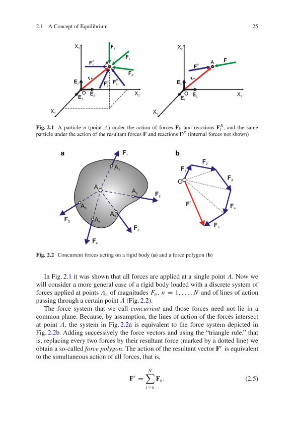
Fig. 2.3 Geometricalinterpretation of thethree-forces theorem
The method of construction of a force polygon indicates that in order to obtainvector Fr we can add the vectors Fn together directly (i.e., the vectors denoted bydotted lines can be omitted during addition).
The vectors Fn are called sides of a force polygon and the vector Fr is called aclosing vector of a force polygon. Moreover, the sign of the sum (sigma) denotesaddition of vectors from left to right, that is, from F1; F2; : : : to FN .
The presented construction is easy in the case of a planar force system. In space,the force polygon is a broken line whose sides are the force vectors and the resultantFr connects the tail of the first force vector to the tip of the last force vector of thegiven force system. In this section we will take up the analysis of the planar forcepolygon.
From the foregoing considerations it follows directly that because the actionof many forces can be replaced by the action of one resultant force, a rigid bodyremains in equilibrium under the action of a concurrent force system if Fr D 0, thatis, according to (2.5) if
NX
nD1Fn D 0: (2.6)
If the above equation is satisfied, the polygon of forces Fn is closed, that is, thetail of the first force vector coincides with the tip of the last force vector.
Theorem 2.2. (On three forces) If a body remains in equilibrium under the actionof only three non-parallel coplanar forces, then their lines of action must intersectat a single point, that is, the system of forces must be concurrent.
To prove the above theorem it is enough to observe that if we have three forcesF1, F2, and F3, then the action of any two of them, e.g., F1 and F2, can be replacedwith their resultant Fr . According to Newton’s first law, the body is in equilibriumif Fr D �F3 and these vectors are collinear. Therefore, the lines of action of thethree forces must intersect at a single point (Fig. 2.3).
Let us note that if we are dealing with a system of three concurrent forces and abody under the action of these forces is in equilibrium, all of these forces must becoplanar (i.e., lie in one plane).
Later we will show (by making use of Theorem 2.2) how to reduce an arbitrarythree-dimensional system of non-concurrent forces to a so-called equivalent systemof two skew forces.
2.1 A Concept of Equilibrium 27
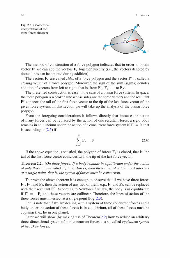
Fig. 2.4 Coordinate systems OX1X2X3 and O 0X 0
1X0
2X0
3 and the force vector F
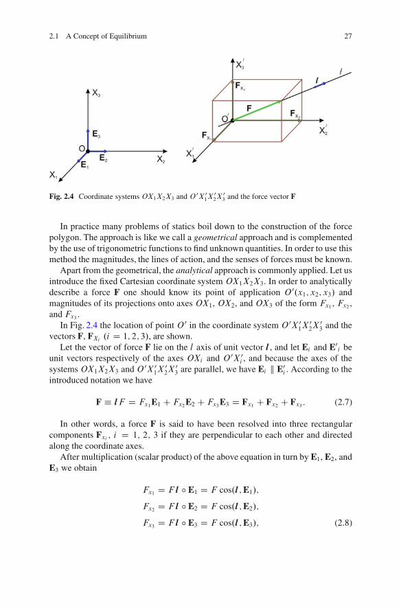
In practice many problems of statics boil down to the construction of the forcepolygon. The approach is like we call a geometrical approach and is complementedby the use of trigonometric functions to find unknown quantities. In order to use thismethod the magnitudes, the lines of action, and the senses of forces must be known.
Apart from the geometrical, the analytical approach is commonly applied. Let usintroduce the fixed Cartesian coordinate system OX1X2X3. In order to analyticallydescribe a force F one should know its point of application O 0.x1; x2; x3/ andmagnitudes of its projections onto axes OX1, OX2, and OX3 of the form Fx1 , Fx2 ,and Fx3 .
In Fig. 2.4 the location of point O 0 in the coordinate system O 0X 01X
02X
03 and the
vectors F, FXi .i D 1; 2; 3/, are shown.Let the vector of force F lie on the l axis of unit vector l , and let Ei and E0
i beunit vectors respectively of the axes OXi and O 0X 0
i , and because the axes of thesystems OX1X2X3 and O 0X 0
1X02X
03 are parallel, we have Ei k E0
i . According to theintroduced notation we have
F � lF D Fx1E1 C Fx2E2 C Fx3E3 D Fx1 C Fx2 C Fx3 : (2.7)
In other words, a force F is said to have been resolved into three rectangularcomponents Fxi ; i D 1; 2; 3 if they are perpendicular to each other and directedalong the coordinate axes.
After multiplication (scalar product) of the above equation in turn by E1, E2, andE3 we obtain
Fx1 D F l ı E1 D F cos.l ;E1/;
Fx2 D F l ı E2 D F cos.l ;E2/;
Fx3 D F l ı E3 D F cos.l ;E3/; (2.8)
28 2 Statics
becausejl j D jE1j D jE2j D jE3j D 1:
If we know the vector F, that is, its magnitude F and direction defined by the unitvector l, the coordinates of the components of the vector are described by (2.8).
After squaring (2.7) by sides we obtain
F DqF 2x1
C F 2x2
C F 2x3; (2.9)
and after taking into account (2.9) in (2.8) we calculate the cosines of the anglesformed by the force vector with the axes of the coordinate system (called directioncosines)
cos.l ;E1/ D Fx1F
D Fx1qF 2x1
C F 2x2
C F 2x3
;
cos.l ;E2/ D Fx2F
D Fx2qF 2x1
C F 2x2
C F 2x3
;
cos.l ;E3/ D Fx3F
D Fx3qF 2x1
C F 2x2
C F 2x3
: (2.10)
If Fx1 , Fx2 and Fx3 are known, then on the basis of (2.9) and (2.10) we candetermine vector F, that is, its magnitude jFj D F and its direction defined by thedirection cosines. It follows directly from (2.10) that cos2.l ;E1/ C cos2.l ;E2/ Ccos2.l ;E3/ D 1, and hence angles describing a position of the force F in relation tothe Cartesian axes depend on each other.
Let us now return to Fig. 2.2, where the system of concurrent forces acts solely onthe rigid body. If such a body is in equilibrium, according to (2.5), we have Fr D 0,and after multiplying (2.5) by E1, E2, and E3 we obtain
F1x1 C F2x1 C � � � C FNx1 D 0;
F1x2 C F2x2 C � � � C FNx2 D 0;
F1x3 C F2x3 C � � � C FNx3 D 0: (2.11)
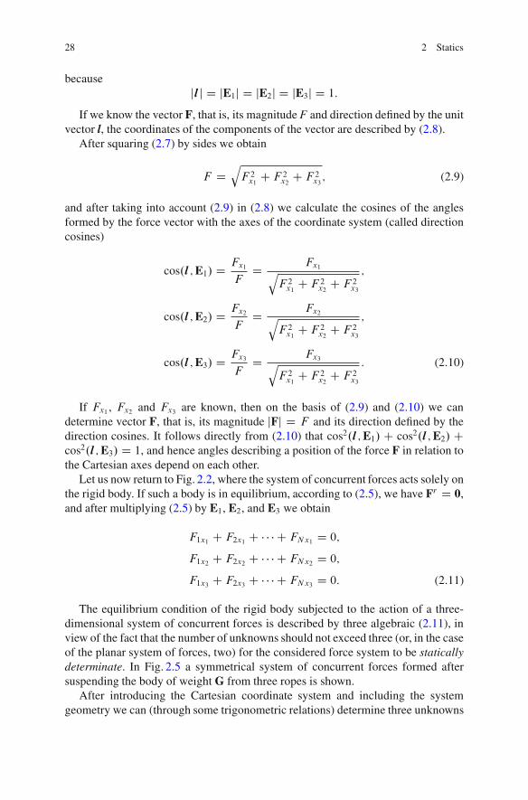
The equilibrium condition of the rigid body subjected to the action of a three-dimensional system of concurrent forces is described by three algebraic (2.11), inview of the fact that the number of unknowns should not exceed three (or, in the caseof the planar system of forces, two) for the considered force system to be staticallydeterminate. In Fig. 2.5 a symmetrical system of concurrent forces formed aftersuspending the body of weight G from three ropes is shown.
After introducing the Cartesian coordinate system and including the systemgeometry we can (through some trigonometric relations) determine three unknowns
2.1 A Concept of Equilibrium 29
Fig. 2.5 A weight Gsuspended from three (four)ropes in space (a) and asystem of concurrentforces (b)
from three equations and, consequently, describe the forces F1, F2, and F3. Let usassume now that at the center O of the triangle ABC an extra fourth rope wasattached. If the length of that rope differs even slightly from the distance h, eitherthat rope exclusively carries the total weight G (if slightly shorter) or it carries noload at all (if slightly longer).
If we assume that the weight G is carried by four ropes, it is impossible todetermine the four forces F1, F2, F3, and F4 in the ropes; such a problem isstatically indeterminate. This appears also in the planar system of concurrent forcesif point C becomes coincident with point B and then AO D OB . The problem isstatically determinate if the weight G is suspended from two ropes AO 0 and BO 0and statically indeterminate if, additionally, we introduce the third ropeOO 0 and allthree ropes are loaded.
One deals with a statically indeterminate problem when the number of unknownvalues of forces (torques) denoted by N is larger than the number of equilibriumequations Nr . The difference N � Nr is called a degree of static indeterminacy.As will be shown later, additional equilibrium equations are obtained after takinginto account deformations of the investigated mechanical system. In general, whilesolving a statically indeterminate problem, the method of forces and the method ofdisplacements are often applied.
The first approach consists of three stages [26]:
1. Determination of degree of static indeterminacy.2. Transformation of a statically indeterminate system to a statically determinate
one with unknown values of loads but known character and point of application.3. Determination of a set of desired force values from condition of displacement
continuity at the force application points.
The second method, i.e., the displacements method, is to use the relationshipbetween external forces, displacement nodes of the construction, displacements ofthe ends of particular ropes (rods) and their geometric and material properties.
30 2 Statics
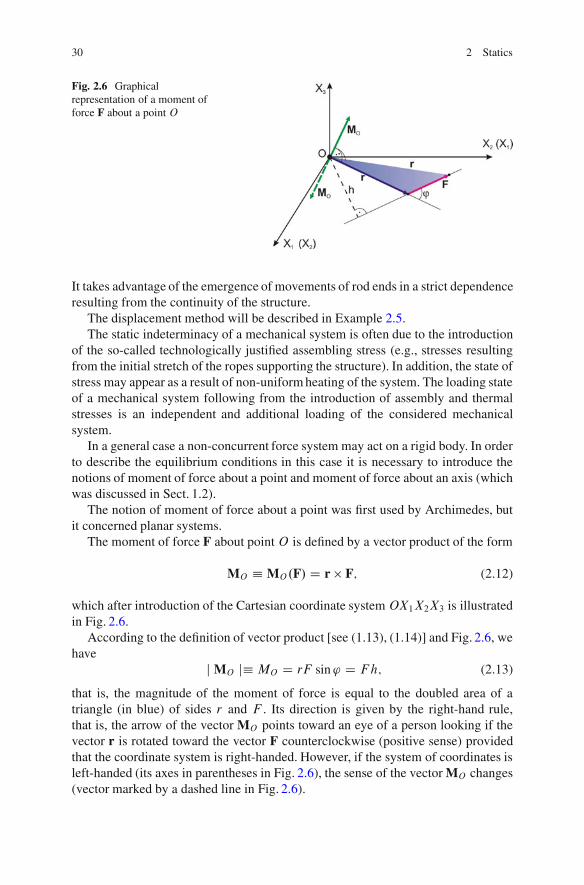
Fig. 2.6 Graphicalrepresentation of a moment offorce F about a point O
It takes advantage of the emergence of movements of rod ends in a strict dependenceresulting from the continuity of the structure.
The displacement method will be described in Example 2.5.The static indeterminacy of a mechanical system is often due to the introduction
of the so-called technologically justified assembling stress (e.g., stresses resultingfrom the initial stretch of the ropes supporting the structure). In addition, the state ofstress may appear as a result of non-uniform heating of the system. The loading stateof a mechanical system following from the introduction of assembly and thermalstresses is an independent and additional loading of the considered mechanicalsystem.
In a general case a non-concurrent force system may act on a rigid body. In orderto describe the equilibrium conditions in this case it is necessary to introduce thenotions of moment of force about a point and moment of force about an axis (whichwas discussed in Sect. 1.2).
The notion of moment of force about a point was first used by Archimedes, butit concerned planar systems.
The moment of force F about point O is defined by a vector product of the form
MO � MO.F/ D r � F; (2.12)
which after introduction of the Cartesian coordinate system OX1X2X3 is illustratedin Fig. 2.6.
According to the definition of vector product [see (1.13), (1.14)] and Fig. 2.6, wehave
j MO j� MO D rF sin' D Fh; (2.13)
that is, the magnitude of the moment of force is equal to the doubled area of atriangle (in blue) of sides r and F . Its direction is given by the right-hand rule,that is, the arrow of the vector MO points toward an eye of a person looking if thevector r is rotated toward the vector F counterclockwise (positive sense) providedthat the coordinate system is right-handed. However, if the system of coordinates isleft-handed (its axes in parentheses in Fig. 2.6), the sense of the vector MO changes(vector marked by a dashed line in Fig. 2.6).
2.1 A Concept of Equilibrium 31
Let us note that vectors describing a real physical quantity (e.g., force, velocity,acceleration) do not change when the adopted coordinate system is changed. In theconsidered case the vector of the moment of force MO changes when the coordinatesystem is changed from right-handed to left-handed. Vectors having such a propertyare called pseudovectors.
Theorem 2.3. (Varignon1) The moment of a resultant force of a system of concur-rent forces about an arbitrary point O (a pole) is equal to the sum of individualmoments of each force of the system about that pole.
Proof of the above theorem is obvious if one uses the property of distributivity ofa vector product with respect to addition.
Let us note that Varignon’s theorem includes also the special case of concurrentforces when the point of intersection of their lines of action is situated in infinity (inthat case we are dealing with a system of parallel forces). Moreover, let us note thatthe introduction of any force F0 of the direction along that of r does not change themoment since we have
MO D r � .F C F0/ D r � F C r � F0 D r � F; (2.14)
because r � F0 D 0.This trivial observation will be exploited later during the reduction of an arbitrary
three-dimensional force system to two skew forces in space (forces that do not liein one plane).
If by a resultant force we understand the force replacing the action of the systemof concurrent forces, such a notion loses its meaning in the case of an arbitrary forcesystem in space. Then the closing vector of a three-dimensional polygon of forcesis called a main force vector.
The components of the moment of force vector about a pole O is obtaineddirectly from the definition using the determinant, that is,
MO D r � F DˇˇˇE1 E2 E3rx1 rx2 rx3Fx1 Fx2 Fx3
ˇˇˇ
D E1.rx2Fx3 � rx3Fx2/C E2.�rx1Fx3 C rx3Fx1/C E3.rx1Fx2 � rx2Fx1/
� MOx1E1 CMOx2E2 CMOx3E3: (2.15)
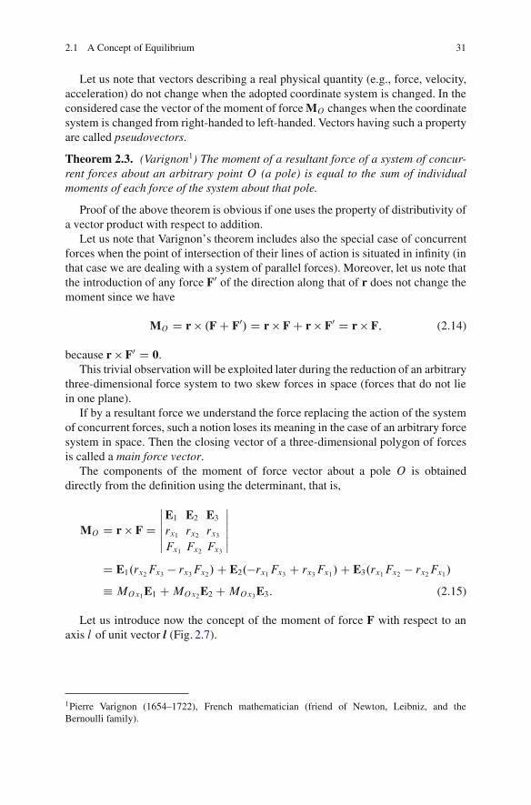
Let us introduce now the concept of the moment of force F with respect to anaxis l of unit vector l (Fig. 2.7).
1Pierre Varignon (1654–1722), French mathematician (friend of Newton, Leibniz, and theBernoulli family).
32 2 Statics
Fig. 2.7 Moment of forceF about an axis l
Definition 2.1. The magnitude of the moment of force about an axis l is equal tothe scalar product of the moment of force about an arbitrary point O on that axisand a unit vector l of the axis (thus it is a scalar that respects the sign determinedby the sense in agreement or opposite to the unit vector l).
According to the above definition, and after taking into account (2.15), we have
Ml.F/ D l ı M0.F/
D MOx1 cos.l ;E1/CMOx2 cos.l ;E2/CMOx3 cos.l ;E3/
D .rx2Fx3 � rx3Fx2/ cos.l ;E1/C .�rx1Fx3 C rx3Fx1/ cos.l ;E2/
C .rx1Fx2 � rx2Fx1/ cos.l ;E3/
Dˇˇˇcos.l ;E1/ cos.l ;E2/ cos.l ;E3/
rx1 rx2 rx3Fx1 Fx2 Fx3
ˇˇˇ : (2.16)
Observe thatMl.F/ is the magnitude of the moment of force about axis l, that is,it depends on the versor l sense.
Let us resolve F.r/ into two rectangular components kF.kr/ and ?F.?r/ (lyingin a plane perpendicular to l ). Then from (2.16) we obtain Ml.F/ D l ı .kr C?r/� .kF C ?F/ D l ı .?r � ?F/. In other words the momentMl.F/ describes thetendency of the force M to give to the rigid body a rotation about the fixed axis l .
At the end of this section we will present definitions of a couple and a momentof a couple and introduce the basic properties of a couple.
Definition 2.2. A system of two parallel forces with opposite senses and equalvalues we call a couple of forces. A plane in which these forces lie is called aplane of a couple of forces.
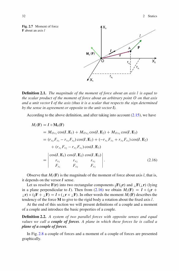
In Fig. 2.8 a couple of forces and a moment of a couple of forces are presentedgraphically.
2.1 A Concept of Equilibrium 33
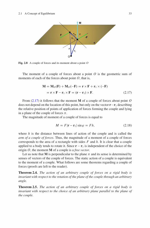
Fig. 2.8 A couple of forces and its moment about a point O
The moment of a couple of forces about a point O is the geometric sum ofmoments of each of the forces about pointO , that is,
M D MO.F/C MO.�F/ D r � F C r1 � .�F/
D r � F � r1 � F D .r � r1/ � F: (2.17)
From (2.17) it follows that the moment M of a couple of forces about point Odoes not depend on the location of this point, but only on the vector r�r1 describingthe relative position of points of application of forces forming the couple and lyingin a plane of the couple of forces � .
The magnitude of moment of a couple of forces is equal to
M D F jr � r1j sin' D Fh; (2.18)
where h is the distance between lines of action of the couple and is called thearm of a couple of forces. Thus, the magnitude of a moment of a couple of forcescorresponds to the area of a rectangle with sides F and h. It is clear that a coupleapplied to a body tends to rotate it. Since r � r1 is independent of the choice of theoriginO , the moment M of a couple is a free vector.
Let us note that M is perpendicular to the plane � and its sense is determined bysenses of vectors of the couple of forces. The static action of a couple is equivalentto the moment of a couple. What follows are some theorems regarding a couple offorces (proofs are left to the reader).
Theorem 2.4. The action of an arbitrary couple of forces on a rigid body isinvariant with respect to the rotation of the plane of the couple through an arbitraryangle.
Theorem 2.5. The action of an arbitrary couple of forces on a rigid body isinvariant with respect to the choice of an arbitrary plane parallel to the plane ofthe couple.
34 2 Statics
Theorem 2.6. The action of an arbitrary couple of forces on a rigid body isinvariant if the product Fh [see (2.18)] remains unchanged, that is, it is possible tovary the magnitude of force and its arm as long as Fh remains constant.
Theorem 2.7. An arbitrary system of couples of forces in R3 space is staticallyequivalent to a single couple of forces whose moment is the geometrical (vector)sum of moments coming from each couple of forces in the system.
The reader is encouraged to prove that two couples possessing the same momentM are equivalent. Since the couples can be presented by vectors, they can besummed up in a geometrical manner. In addition, any given force F acting on arigid body can be resolved into a force at an arbitrary given pole O and a couple,that is, at point O we have an equivalent force–couple .F � MO/ system providedthat the couple’s moment is equal to the moment of F about O . In what follows weapply the statements and comments introduced thus far.
Let us emphasize that the net result of a couple relies on the production of amoment M (couple vector). Since M is independent of the point about which it takesplace (free vector), then in practice it should be computed about a most convenientpoint for analysis. One may add two or more couples in a geometric way. Onemay also replace a force with (a) an equivalent force couple at a specified point;(b) a single equivalent force provided that F ? M, which is satisfied in all two-dimensional problems.
In Fig. 2.1 the position of a particle is described by the vector rn in the adoptedCartesian coordinate system. In the case of a system of particles, each particle nof the system is described by a radius vector rn, n D 1; : : : ;N . After multiplyingequilibrium condition (2.1) by rn (cross product) and adding together the obtainedequations (after assuming Fin D 0) we obtain
MO DNX
nD1.rn � Fn/C
NX
nD1.rn � FRn / D 0: (2.19)
Let us note that (2.19) is also valid for Fin ¤ 0 becausePN
nD1.rn � Fin/ D 0(internal forces of the system exist in pairs that are equal, act along the same lineof action, but have opposite senses; therefore, taken together they all yield zeromoment about any point).
According to (2.4) and (2.19) a material system is in equilibrium if the system offorces and reactions, and the main moment produced by these forces and reactions,is equal to zero, that is, we have
S D 0; MO D 0: (2.20)
Let us note that the above condition is a necessary condition, but in general itis not a sufficient one. According to Newton’s first law, particles can move along
2.1 A Concept of Equilibrium 35
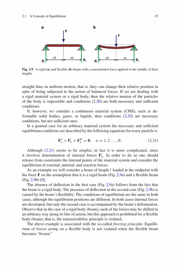
Fig. 2.9 A rigid (a) and flexible (b) beam with a concentrated force applied in the middle of theirlengths
straight lines in uniform motion, that is, they can change their relative position inspite of being subjected to the action of balanced forces. If we are dealing witha rigid material system or a rigid body, then the relative motion of the particlesof the body is impossible and conditions (2.20) are both necessary and sufficientconditions.
If, however, we consider a continuous material system (CMS), such as de-formable solid bodies, gases, or liquids, then conditions (2.20) are necessaryconditions, but not sufficient ones.
In a general case for an arbitrary material system the necessary and sufficientequilibrium conditions are described by the following equations for every particle n:
Fen C Fin C FRn D 0; n D 1; 2 : : : ; N: (2.21)
Although (2.21) seems to be simpler, in fact it is more complicated, sinceit involves determination of internal forces Fin. In order to do so one shouldrelease from constraints the internal points of the material system and consider theequilibrium of external, internal, and reaction forces.
As an example we will consider a beam of length l loaded at the midpoint withthe force F on the assumption that it is a rigid beam (Fig. 2.9a) and a flexible beam(Fig. 2.9b) [9].
The absence of deflection in the first case (Fig. 2.9a) follows from the fact thatthe beam is a rigid body. The presence of deflection in the second case (Fig. 2.9b) iscaused by the beam’s flexibility. The conditions of equilibrium are the same in bothcases, although the equilibrium positions are different. In both cases internal forcesare developed, but only the second case is accompanied by the beam’s deformation.Observe that in the case of a rigid body (beam), each of the forces may be shifted inan arbitrary way along its line of action, but this approach is prohibited for a flexiblebody (beam), that is, the transmissibility principle is violated.
The above example is associated with the so-called freezing principle. Equilib-rium of forces acting on a flexible body is not violated when the flexible beambecomes “frozen.”
36 2 Statics
2.2 Geometrical Equilibrium Conditions of a Planar ForceSystem
As has already been mentioned, in a general case formulation of geometricalequilibrium conditions is not an easy problem, and usually this approach is appliedto systems of forces lying in a plane. As was shown earlier, according to the firstequation of (2.20) a polygon constructed from force vectors should be closed.
In the case where a material system is acted upon by a system of three non-parallel forces equivalent to zero, these forces are coplanar and their lines of actionintersect at one point, forming a triangle (Theorem 2.2).
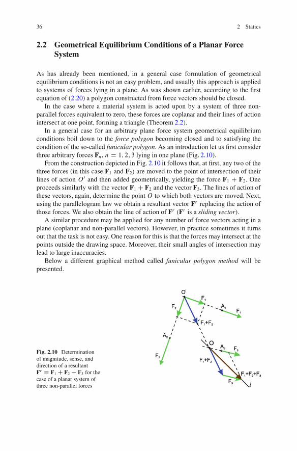
In a general case for an arbitrary plane force system geometrical equilibriumconditions boil down to the force polygon becoming closed and to satisfying thecondition of the so-called funicular polygon. As an introduction let us first considerthree arbitrary forces Fn, n D 1; 2; 3 lying in one plane (Fig. 2.10).
From the construction depicted in Fig. 2.10 it follows that, at first, any two of thethree forces (in this case F1 and F2) are moved to the point of intersection of theirlines of action O 0 and then added geometrically, yielding the force F1 C F2. Oneproceeds similarly with the vector F1 C F2 and the vector F3. The lines of action ofthese vectors, again, determine the point O to which both vectors are moved. Next,using the parallelogram law we obtain a resultant vector Fr replacing the action ofthose forces. We also obtain the line of action of Fr (Fr is a sliding vector).
A similar procedure may be applied for any number of force vectors acting in aplane (coplanar and non-parallel vectors). However, in practice sometimes it turnsout that the task is not easy. One reason for this is that the forces may intersect at thepoints outside the drawing space. Moreover, their small angles of intersection maylead to large inaccuracies.
Below a different graphical method called funicular polygon method will bepresented.
Fig. 2.10 Determinationof magnitude, sense, anddirection of a resultantFr D F1 C F2 C F3 for thecase of a planar system ofthree non-parallel forces
2.2 Geometrical Conditions (Planar System) 37
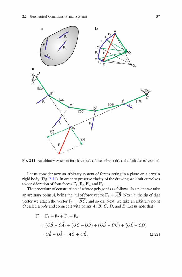
Fig. 2.11 An arbitrary system of four forces (a), a force polygon (b), and a funicular polygon (c)
Let us consider now an arbitrary system of forces acting in a plane on a certainrigid body (Fig. 2.11). In order to preserve clarity of the drawing we limit ourselvesto consideration of four forces F1, F2, F3, and F4.
The procedure of construction of a force polygon is as follows. In a plane we take
an arbitrary point A, being the tail of force vector F1 D ��!AB . Next, at the tip of that
vector we attach the vector F2 D ��!BC , and so on. Next, we take an arbitrary point
O called a pole and connect it with points A; B; C; D, and E . Let us note that
Fr D F1 C F2 C F3 C F4
D ���!OB � �!
OA�C ���!
OC � ��!OB
�C ���!OD � ��!
OC�C ���!
OE � ��!OD
�
D ��!OE � �!
OA D ��!AO C ��!
OE: (2.22)
38 2 Statics
The segments OA; OB; OC; OD, and OE are called rays, but in (2.10) the
vectors of their lengths appeared as forces, which means j�!OAj D OA, and so on.
The force polygon allows for determination of the resultant Fr , that is, the forcereplacing the action of forces F1; F2; F3, and F4. However, additionally we have todetermine the line of action of the resultant force (it must be parallel to the directionof the force Fr obtained using the force polygon method, see Fig. 2.11b). In practicethis means that one should determine a point W through which the force Fr wouldpass.
To this end we make use of the so-called funicular polygon. Let us take anarbitrary point A0 lying on the line of action of the force F1 (construction istemporarily conducted in a separate drawing). Next, we draw a line passing throughthat point and parallel to OA (cf. the force polygon). Then, we step off on that
line a segment A0B 0 of length j��!AOj (one may limit oneself to the determination ofthe direction of that force). Next, through point B 0 we draw a line parallel to OB
and step off the segment B 0C 0 D j��!OBj. Through the obtained point C 0 we draw
a line parallel to OC and step off the segment C 0D0 D j��!OC j, obtaining in thisway point D0. Through that point we draw a line parallel to OD and step off the
segment D0E 0 D j��!ODj. Through the obtained point E 0 we draw a line parallel to
OE and step off the segment E 0O 0 D j��!EOj. According to (2.22) the resultant can
be determined using the parallelogram law, since the force vectors��!AO and
��!OE are
known [the forces represented by the other vectors (rays) cancel each other]. One
may also move the vectors��!AO and
��!OB ,
��!BO and
��!OC ,
��!CO and
��!OD respectively
to points B 0; C 0;D0, and E 0. It is easy to notice that after their geometrical addition
only the vectors��!AO and
��!OE remain. It follows that extending the lines passing
through points A0 and B 0, and through O 0 and E 0, leads to determination of pointW , through which passes the line of action of the resultant Fr . It follows also thatit is possible to determine the magnitude of that force (after geometrical addition of
j���!A0B 0j and j���!
O 0E 0j).If we took a perfectly flexible cable of negligible weight and lengthAOCOBC
OCCODCOE and fixed it at pointsA0 andO 0, then after application of the forcesF1, F2, F3, and F4 at points B 0, C 0,D0, and E 0 (Fig. 2.11c), the cable would remainin equilibrium. That is where the name of funicular polygon comes from. At eachof these points act three forces that are in equilibrium. It is easy to check that thechoice of some other pole (point O1 in Fig. 2.11b) leads to the determination of adifferent point of intersection, but it must lie on the line of action of the force Fr .
Let us now consider the particular case of the force polygon depicted inFig. 2.11b, namely, when Fr ! 0, that is, when E ! A, which means that
j��!EOj D j�!OAj and the vectors
��!OE and
��!AO become collinear at the limit while
retaining the opposite senses. Since the polygonABCDA is closed, pointsA andEare coincident, that is, A � E .
Such a situation is depicted in Fig. 2.12a, and the corresponding force polygon isshown in Fig. 2.12b.
2.2 Geometrical Conditions (Planar System) 39
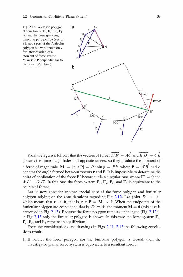
Fig. 2.12 A closed polygonof four forces F1, F2, F3, F4(a) and the correspondingfunicular polygon (b) (vectorr is not a part of the funicularpolygon but was drawn onlyfor interpretation of amoment of force vectorM D r � P perpendicular tothe drawing’s plane)
From the figure it follows that the vectors of forces���!A0B 0 D ��!
AO and���!E 0O 0 D ��!
OE
possess the same magnitudes and opposite senses, so they produce the moment of
a force of magnitude jMj D jr � Pj D P r sin' D Ph, where P D ���!A0B 0 and '
denotes the angle formed between vectors r and P. It is impossible to determine thepoint of application of the force Fr because it is a singular case where Fr D 0 andA0B 0 k O 0E 0. In this case the force system F1, F2, F3, and F4 is equivalent to thecouple of forces.
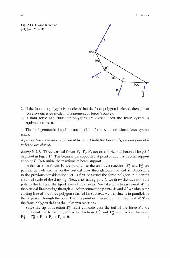
Let us now consider another special case of the force polygon and funicularpolygon relying on the considerations regarding Fig. 2.12. Let point E 0 ! A0,which means that r ! 0, that is, r � P D M ! 0. When the endpoints of thefunicular polygon are coincident, that is, E 0 � A0, the moment M D 0 (this case ispresented in Fig. 2.13). Because the force polygon remains unchanged (Fig. 2.12a),in Fig. 2.13 only the funicular polygon is shown. In this case the force system F1,F2, F3, and F4 remains in equilibrium.
From the considerations and drawings in Figs. 2.11–2.13 the following conclu-sions result:
1. If neither the force polygon nor the funicular polygon is closed, then theinvestigated planar force system is equivalent to a resultant force.
40 2 Statics
Fig. 2.13 Closed funicularpolygon (M D 0)
2. If the funicular polygon is not closed but the force polygon is closed, then planarforce system is equivalent to a moment of force (couple).
3. If both force and funicular polygons are closed, then the force system isequivalent to zero.
The final geometrical equilibrium condition for a two-dimensional force systemreads:
A planar force system is equivalent to zero if both the force polygon and funicularpolygon are closed.
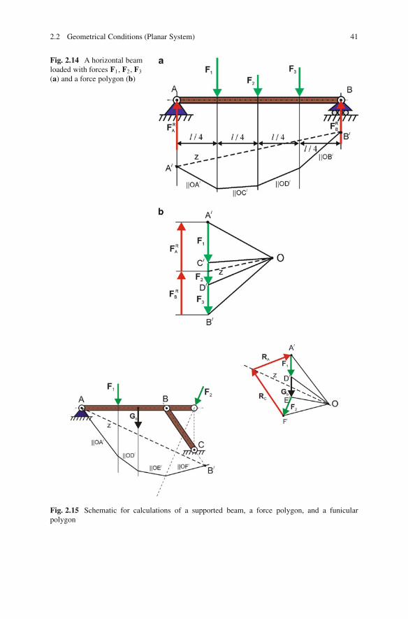
Example 2.1. Three vertical forces F1, F2, F3 act on a horizontal beam of length ldepicted in Fig. 2.14. The beam is pin supported at point A and has a roller supportat point B . Determine the reactions in beam supports.
In this case the forces Fn are parallel, so the unknown reactions FRA and FRB areparallel as well and lie on the vertical lines through points A and B . Accordingto the previous considerations let us first construct the force polygon in a certainassumed scale of the drawing. Next, after taking pole O we draw the rays from thepole to the tail and the tip of every force vector. We take an arbitrary point A0 onthe vertical line passing throughA. After connecting pointsA0 and B 0 we obtain theclosing line of the force polygon (dashed line). Next, we translate it in parallel, sothat it passes through the pole. Then its point of intersection with segment A0B 0 inthe force polygon defines the unknown reactions.
Since the tip of reaction FRA must coincide with the tail of the force F1, wecomplement the force polygon with reactions FRA and FRB and, as can be seen,FRA C FRB C F1 C F2 C F3 D 0. ut
2.2 Geometrical Conditions (Planar System) 41
Fig. 2.14 A horizontal beamloaded with forces F1, F2, F3(a) and a force polygon (b)
Fig. 2.15 Schematic for calculations of a supported beam, a force polygon, and a funicularpolygon
42 2 Statics
Example 2.2. A horizontal beam is loaded with forces F1 and F2 (Fig. 2.15). Thebeam is pin supported at point A and at point B supported by the rod with a pinjoint. Determine the reactions in pin joints A and C assuming that the beam has ahomogeneous mass distribution and weight Gb .
Because in this case only the vectors F1 and Gb are parallel to each other but arenot parallel to F2, the reactions FRA and FRC are not parallel (the direction of reactionFRC is defined by the axis of rodBC ). We construct the force polygon for F1, Gb , F2.
The construction of the funicular polygon we start from point A (reaction FRAmust pass through point A, but its direction is unknown). Doing the construction inthe way described earlier, the line parallel to OF 0 intersects segment BC at pointB 0 and segment AB 0 is the closing line of the funicular polygon. After drawing aline parallel to AB 0 that passes through pole O (line z) and drawing from the tip ofthe vector F2 the line parallel to BC , the point of their intersection determines theunknown reactions FRA and FRC . ut
2.3 Geometrical Equilibrium Conditions of a Space ForceSystem
As distinct from the previously analyzed case of the concurrent force system shownin Fig. 2.2, we will consider now a non-concurrent force system.
Our aim is to reduce the force system F1; : : : ;FN to an arbitrary chosen pointOof the body (or rigidly connected to the body) called a pole.
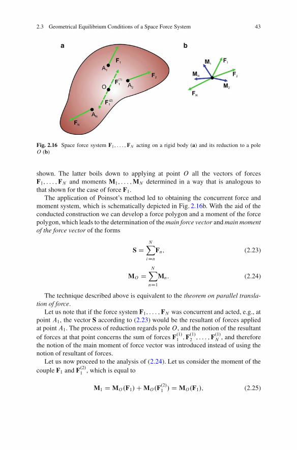
The method given below was presented already by Poinsot2 and henceforth iscalled Poinsot’s method. We will show that, according to Poinsot’s method, theaction of the force F1 on a rigid body with respect to pole O is equivalent to theaction of the force F1 applied at point O and a couple F1 and F.2/1 applied at points
A1 andO , respectively, and F.2/1 D �F1.In other words at point O we apply the forces F.1/1 and F.2/1 , where F.1/1 denotes
the vector F1 moved in a parallel translation to point O , and F.2/1 D �F.1/1 . Point Ois in equilibrium under the action of two vectors of the directions along the directionof F1 and having the same magnitudes but opposite senses.
The action of force at point A1 manifests at pointO as the action of the force F1at that point and the couple F1 (applied at point A1) and �F1 (applied at point O).In turn, the action of the couple F1 and �F1 is equivalent to the action of a moment
of the couple, which according to (2.17) is equal to M1 D ��!OA1 � F1.
In Fig. 2.16a at point O only the two forces F.1/1 and F.2/1 canceling one anotherare marked, and in Fig. 2.16b reduction of the whole force system F1; : : : ;FN is
2Louis Poinsot (1777–1859), French mathematician and physicist, precursor of geometricalmechanics.
2.3 Geometrical Equilibrium Conditions of a Space Force System 43
Fig. 2.16 Space force system F1; : : : ;FN acting on a rigid body (a) and its reduction to a poleO (b)
shown. The latter boils down to applying at point O all the vectors of forcesF1; : : : ;FN and moments M1; : : : ;MN determined in a way that is analogous tothat shown for the case of force F1.
The application of Poinsot’s method led to obtaining the concurrent force andmoment system, which is schematically depicted in Fig. 2.16b. With the aid of theconducted construction we can develop a force polygon and a moment of the forcepolygon, which leads to the determination of the main force vector and main momentof the force vector of the forms
S DNX
iDnFn; (2.23)
MO DNX
nD1Mn: (2.24)
The technique described above is equivalent to the theorem on parallel transla-tion of force.
Let us note that if the force system F1; : : : ;FN was concurrent and acted, e.g., atpoint A1, the vector S according to (2.23) would be the resultant of forces appliedat point A1. The process of reduction regards poleO , and the notion of the resultantof forces at that point concerns the sum of forces F.1/1 ;F
.1/2 ; : : : ;F
.1/N , and therefore
the notion of the main moment of force vector was introduced instead of using thenotion of resultant of forces.
Let us now proceed to the analysis of (2.24). Let us consider the moment of thecouple F1 and F.2/1 , which is equal to
M1 D MO.F1/C MO.F.2/1 / D MO.F1/; (2.25)
44 2 Statics
because the force F.2/1 passes through pole O . Similar considerations concern theremaining forces, and finally (2.24) takes the following form:
MO DNX
nD1MO.Fn/: (2.26)
The result of the considerations carried out above leads to the formulation of thegeneral theorem of statics of a rigid body.
Theorem 2.8. An arbitrary system of non-concurrent forces in space acting ona rigid body is statically equivalent to the action of the main force vector (2.23)applied at an arbitrary point (pole) and the main moment of force vector (2.24).
2.4 Analytical Equilibrium Conditions
An analytical form of equilibrium conditions relies on the vectorial (2.20). Becausein the Euclidean space each of the vectors possesses three projections, the equilib-rium conditions boil down to the following three conditions concerning the forces:
Sxj DNX
nD1Fxj n D 0; j D 1; 2; 3; (2.27)
and because
MO DNX
nD1.rn � Fn/ D
NX
nD1
ˇˇˇ
E1 E2 E3x1n x2n x3nFx1n Fx2n Fx3n
ˇˇˇ
DNX
nD1
hE1�x2nFx3n � x3nFx2n
�C E2�x3nFx1n � x1nFx3n
�
C E3�x1nFx2n � x2nFx1n
�i; (2.28)
we have an additional three equilibrium equations of the form
MOx1 �NX
nD1
�x2nFx3n � x3nFx2n
� D 0;
MOx2 �NX
nD1
�x3nFx1n � x1nFx3n
� D 0;
MOx3 �NX
nD1
�x1nFx2n � x2nFx1n
� D 0; (2.29)
2.4 Analytical Equilibrium Conditions 45
where MO D P3jD1 EjMOxj . In general, the main moment changes with a change
of the reduction point (the pole).From the equations above it follows that the force system of the lines of action
laid out arbitrarily in space is in equilibrium if the algebraic equations (2.27)and (2.29) are satisfied. From the mentioned equations it is easy to obtain therelations regarding the forces lying in the selected planes .O � X1 � X2/ or.O � X1 � X3/. In the equations above the forces Fn denote external forces andreactions.
External forces can be divided into concentrated forces (applied to points of abody), surface forces (applied over certain areas), and volume forces (applied toall particles of a body). An example of volume forces are the forces caused by thebody weight, and of surface forces—the forces generated by the surface of contactbetween the bodies being loaded. A set of external forces consists of known forces(active forces) and the forces that are subject to determination (passive forces).
The set of external (active and passive) forces is called the loading of amechanical system.
Let us consider a wheeled vehicle (a car with four wheels) with an extra loadplaced on its roof. Here the active forces are the car weight Gc and load weightGl . At the points of contact between each wheel and road surface appear fourreactions FRi . Here the external forces are the forces Gc and Gl (active forces)and reactions FRi (passive forces). The remaining forces acting within the systemisolated from its environment (i.e., the car and load) are called internal forces.According to Newton’s third law these forces mutually cancel each other, and fortheir determination it is necessary to employ the so-called imaginary cut technique.For instance, in order to examine the action of the load on the car one should“cut” the system at the points of contact of the load with the car and replace theirinteraction with reactions, which are the internal forces. Thus we carry out theimaginary division of the analyzed mechanical system into two subsystems in staticequilibrium. Then, from the equilibrium equations of either subsystem we determinethe desired internal forces.
In order to determine the analytical equilibrium conditions one may also makeuse of the so-called three-moments theorem.
Theorem 2.9. If we choose three different non-collinear points Aj , then theequilibrium conditions of a material system are
MAj D MAj
NX
nD1Fn
!D 0; j D 1; 2; 3: (2.30)
This means that the main moment of force vectors of the force system aboutthree arbitrary but non-collinear points are equal to zero. The proof follows. Let theequation be satisfied forA1 (the moment about that point equals zero) and equationsfor two other points not be satisfied. This means that the system is not equivalent tothe couple but to the resultant force that must pass through point A1.
46 2 Statics
Now let two equations of moments about points A1 and A2 be satisfied. Becauseit is possible to draw a line through points A1 and A2, a non-zero resultant forcemust lie on that line. However, if additionally the third equation related to point A3is satisfied and points A1, A2, and A3 are not collinear (by assumption), then theresultant force must be equal to zero. That completes the proof.
Projecting the moments of forces (2.30) on the three axes of Cartesian coordinatesystem we obtain nine algebraic equations of the form
MxnAj D 0; n; j D 1; 2; 3: (2.31)
Here, we are dealing with the apparent contradiction because there are nine (2.31)and six (2.27) and (2.29). However, for (2.31), for each force nine coordinatesdefining its distance from the chosen points A1, A2, and A3 are needed. In therigid body the distances A1A2, A2A3, and A1A3 are constant, which reduces thenumber of independent coordinates to six. So, one may proceed in a different way.The six mutually independent axes should be taken in such a way as to formulatesix independent equations only.
The equilibrium conditions (2.27) and (2.29) consisting of six equations resultedfrom projecting the main force vector S, and the main moment of force vector MO
reduced to an arbitrary point O (Sect. 2.3), where the point of reduction O is theorigin of the Cartesian coordinate system.
The state of equilibrium of the considered rigid body means that it does notmake any displacement, that is, neither translation nor rotation about point O andconsequently with respect to the adopted coordinate system OX1X2X3. We assumethat in the absence of forces F1; : : : ;FN the rigid body does not move with respectto the adopted coordinate system OX1X2X3, and also remains unmoved under theaction of the force system F1; : : : ;FN if (2.27) and (2.29) are satisfied. If under theaction of an arbitrary force system F1; : : : ;FN the rigid body remains in equilibriumwith respect to OX1X2X3, these forces must satisfy (2.27) and (2.29). Since, ifS ¤ 0, MO D 0, point O would be subjected to an action of the force S leading tothe loss of static equilibrium state.
If we had S D 0, MO ¤ 0, then the main moment MO would cause the rotationof the rigid body, leading to the loss of its static equilibrium. Equilibrium equationsof the form
S D F1 C F2 C : : :C FN D 0;
MO D MO.F1/C MO.F2/C : : :C MO.FN / D 0 (2.32)
represent the necessary and sufficient equilibrium conditions for a free (uncon-strained) rigid body subjected to the action of an arbitrary three-dimensional forcesystem. The above conditions transform into conditions (2.27) and (2.29) after theintroduction of the Cartesian coordinate system of origin at O .
In other words, if we reduce an arbitrary three-dimensional system of forcesFn applied at the points An.x1n; x2n; x3n/, n D 1; : : : ; N to an arbitrary point
2.4 Analytical Equilibrium Conditions 47
(the reduction pole) O , we obtain the main force vector S and main moment offorce vector MO , and after adopting the Cartesian coordinate system at pointO , wehave
S D E1NX
nD1F1n C E2
NX
nD1F2n C E3
NX
nD1F3n
D E1S1 C E2S2 C E3S3; (2.33)
and
MO D E1NX
nD1ŒF3n.x2n � x20/ � F2n.x3n � x30/�
C E2NX
nD1ŒF1n.x3n � x30/� F3n.x1n � x10/�
C E3NX
nD1ŒF2n.x1n � x10/ � F1n.x2n � x20/�
� E1M01 C E2M02 C E3M03: (2.34)
In the case of reduction of a three-dimensional force system there exist tworeduction invariants. The first is the main vector S and the second the projectionof vector MO onto the direction of the vector S. The first invariant means that thereduction of spatial forces being in fact a geometrical addition of vectors gives thesame result for an arbitrarily chosen point of reduction. The second invariant meansthat for the arbitrarily chosen point of reduction the projection of the main momentvector onto the direction of the main force vector is constant.
In the latter case it is possible to find such a direction (a straight line) whereif the points of reduction lie on that line, the magnitude of MO is minimum. Onthat line we can place the vector S, which as the invariant may be freely moved inspace. Such a line, after assigning to it the sense defined by the sense of S, we callthe central axis (axis of a wrench). Every set of force vectors and moment of forcevectors can have only one central axis. The system of two vectors S and MO lyingon the central axis we call a wrench.
The general equilibrium conditions (2.27) and (2.29) may be simplified and thenboil down to the special cases of the field of forces considered earlier, which we willbriefly describe below.
A concurrent force system in space. Taking pole O at the point of intersectionof the lines of action of these forces, (2.29) are identically equal to zero, and theequilibrium conditions are described only by three equations (2.27).
48 2 Statics
An arbitrary force system in a plane. An arbitrary planar force system maybe reduced to the main force vector S and main moment of force vector MO .After choosing the axis OX3 perpendicular to the plane of action of the forces theproblem of determination of static equilibrium reduces to the analysis of algebraicequations of the form
S1 DNX
nD1F1n D 0; S2 D
NX
nD1F2n D 0;
MO3 DNX
nD1MO3n.Fn/ D 0: (2.35)
A system of parallel forces in space. Let the axisOX3 be perpendicular to the vectorfield of parallel forces. From (2.27) and (2.29) for the considered case we obtain
NX
nD1F3n D 0;
NX
nD1MO1n.Fn/ D 0;
NX
nD1MO2n.Fn/ D 0: (2.36)
The last case will be analyzed in more detail because we are going to refer to itby the introduction of the notion of a mass center of a system of particles and a masscenter of a rigid body.
In the general case an arbitrary force system acting on a rigid body is equivalentto either an action of main force vector or main moment of force vector.
Up to this point the equivalence of two force systems (sets of forces) wasformulated in a descriptive way. The criterion of equivalence can, however, be statedas a theorem.
Theorem 2.10. The necessary and sufficient condition of equivalence of two forcesystems, acting on a rigid body, with respect to a certain point (pole) is that thesesystems have identical main force vectors and main moment of force vectors withrespect to that point.
The above theorem can be proved based on the principle of virtual work [27].The system of parallel forces in three dimensions includes four special cases:
1. The forces may lie on parallel lines and possess opposite senses and differentmagnitudes.
2. The forces may lie on parallel lines and possess opposite senses but the samemagnitudes.
3. The forces may lie on parallel lines and possess the same senses but differentmagnitudes.
4. The forces may lie on parallel lines and possess the same senses and magnitudes.
Let us limit our considerations to two forces representing the cases listed above.These forces always lie in one plane as they are parallel.
2.4 Analytical Equilibrium Conditions 49
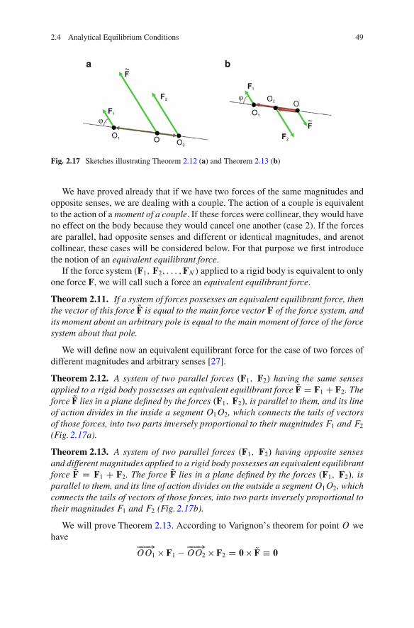
Fig. 2.17 Sketches illustrating Theorem 2.12 (a) and Theorem 2.13 (b)
We have proved already that if we have two forces of the same magnitudes andopposite senses, we are dealing with a couple. The action of a couple is equivalentto the action of a moment of a couple. If these forces were collinear, they would haveno effect on the body because they would cancel one another (case 2). If the forcesare parallel, had opposite senses and different or identical magnitudes, and arenotcollinear, these cases will be considered below. For that purpose we first introducethe notion of an equivalent equilibrant force.
If the force system (F1; F2; : : : ;FN ) applied to a rigid body is equivalent to onlyone force F, we will call such a force an equivalent equilibrant force.
Theorem 2.11. If a system of forces possesses an equivalent equilibrant force, thenthe vector of this force QF is equal to the main force vector F of the force system, andits moment about an arbitrary pole is equal to the main moment of force of the forcesystem about that pole.
We will define now an equivalent equilibrant force for the case of two forces ofdifferent magnitudes and arbitrary senses [27].
Theorem 2.12. A system of two parallel forces .F1; F2/ having the same sensesapplied to a rigid body possesses an equivalent equilibrant force QF D F1 C F2. Theforce QF lies in a plane defined by the forces .F1; F2/, is parallel to them, and its lineof action divides in the inside a segment O1O2, which connects the tails of vectorsof those forces, into two parts inversely proportional to their magnitudes F1 and F2(Fig. 2.17a).
Theorem 2.13. A system of two parallel forces .F1; F2/ having opposite sensesand different magnitudes applied to a rigid body possesses an equivalent equilibrantforce QF D F1 C F2. The force QF lies in a plane defined by the forces .F1; F2/, isparallel to them, and its line of action divides on the outside a segmentO1O2, whichconnects the tails of vectors of those forces, into two parts inversely proportional totheir magnitudes F1 and F2 (Fig. 2.17b).
We will prove Theorem 2.13. According to Varignon’s theorem for point O wehave
���!OO1 � F1 � ���!
OO2 � F2 D 0 � QF � 0
50 2 Statics
and
QF D F1 C F2:
From the first equation it follows for both cases that after passing to scalars wehave
j���!OO1j � jF1j sin ' � j���!
OO2j � jF2j sin.180ı � '/ D 0;
that is,
jOO1j � jF1j D jOO2j � jF2j:Let us consider now the special case that follows from Fig. 2.17b, that is, when
F1 is applied at point O1 and at point O2 the force F2 D �F1, that is, we aredealing with a couple of forces. It is easy to observe that a couple does not possessan equivalent equilibrant force because QF D F1 � F1 D 0. The couple (F1;F2) doeshave, however, a different interesting property, which we have already mentioned.The moment produced by the couple depends not on the choice of the pole in space,but only on the distance of the points of application of the forces F1 and F2 D �F1.It is possible to prove that couples having the same moment of force are equivalentcouples.
Let us now consider the mixed (hybrid) case of a system of parallel forces inspace acting on a rigid body, where some forces have opposite senses and some thesame senses.
As was considered earlier on examples of two parallel forces having either thesame or opposite senses, we can reduce the whole system of parallel forces to twoparallel forces QF1 and QF2, called an equivalent equilibrant force.
The force vectors Fn, n D 1; : : : ; N we will treat as bound vectors (as distinctfrom the free vectors used so far), and the force QF1 represents an equivalentequilibrant force for the forces having senses opposite to the force QF2, replacingthe action of the second group of forces. Finally, the problem of reduction in thiscase is reduced to the problem presented in Fig. 2.17b, which means that we are ableto determine the location of the pointO D C , where an equivalent equilibrant force( QF1; QF2) is applied.
The case depicted in Fig. 2.17b enables us to draw certain further conclusions.Let us observe that according to the proof of Theorem 2.13 at the point O D C ,
the vector of force QF D QF1 C QF2 (Fig. 2.18) is applied and the location of thatpoint depends exclusively on the magnitudes of force vectors, that is, from F1=F2.It follows that the locations of points C , O1, and O2 do not change at the rotationof force vectors through the same angle ˛. Let, after the rotation through the sameangle ˛, the lines of action of the mentioned forces be parallel to the axis OX2 ofthe adopted Cartesian coordinate system, that is, all the previously mentioned forcesafter reduction lie in a plane parallel to the planeOX1X2.
Let us write an equation of moments about an axis OX3 (perpendicular to theplane of the drawing in which the forces lie).
If the number of parallel forces is N , then we will denote them as F1;F2; : : : ;FN , where those having senses opposite to the positive direction of the axis OX2
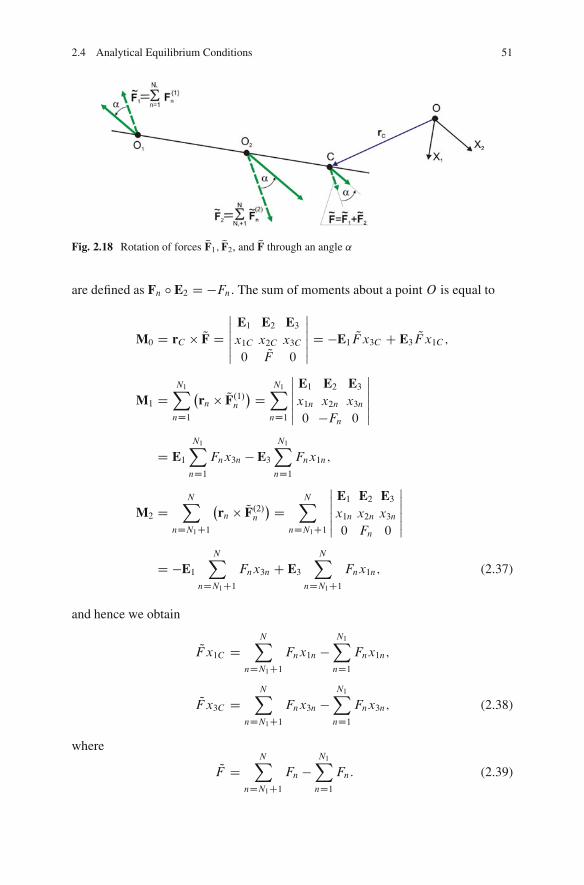
2.4 Analytical Equilibrium Conditions 51
Fig. 2.18 Rotation of forces QF1; QF2, and QF through an angle ˛
are defined as Fn ı E2 D �Fn. The sum of moments about a point O is equal to
M0 D rC � QF Dˇˇˇ
E1 E2 E3x1C x2C x3C0 QF 0
ˇˇˇ D �E1 QFx3C C E3 QFx1C ;
M1 DN1X
nD1
�rn � QF.1/n
� DN1X
nD1
ˇˇˇ
E1 E2 E3x1n x2n x3n0 �Fn 0
ˇˇˇ
D E1N1X
nD1Fnx3n � E3
N1X
nD1Fnx1n;
M2 DNX
nDN1C1
�rn � QF.2/n
� DNX
nDN1C1
ˇˇˇ
E1 E2 E3x1n x2n x3n0 Fn 0
ˇˇˇ
D �E1NX
nDN1C1Fnx3n C E3
NX
nDN1C1Fnx1n; (2.37)
and hence we obtain
QFx1C DNX
nDN1C1Fnx1n �
N1X
nD1Fnx1n;
QFx3C DNX
nDN1C1Fnx3n �
N1X
nD1Fnx3n; (2.38)
where
QF DNX
nDN1C1Fn �
N1X
nD1Fn: (2.39)
52 2 Statics
If we deal only with N parallel forces (we assume N1 D 0) of the same senses,from (2.38) we obtain
NX
nD1Fn
!x1C D
NX
nD1Fnx1n;
NX
nD1Fn
!x3C D
NX
nD1Fnx3n; (2.40)
which defines the position of the center C of the parallel forces having the samesenses consistent with the sense of E2 in the adopted coordinate system.
The third missing equation is
NX
nD1Fn
!x2C D
NX
nD1Fnx2n;
which allows us, through the suitable choice of two out of the three presentedequations, to determine the position of the center of parallel forces in each of theplanes OX1X2, OX2X3, andOX1X3.
If now in the selected points n D 1; : : : ; N we apply the vectors of parallel forcesmng (weights), where g is the acceleration of gravity, we can determine the center ofgravity of those forces after introducing the Cartesian coordinate system such thatFn D mngE3.
The gravity center is coincident with the mass center of the given discretemechanical system in the gravitational field.
Equation (2.40) listed above can be obtained from the following equation:
rC �NX
nD1Fn D
NX
nD1rn � Fn: (2.41)
2.5 Mechanical Interactions, Constraints, and Supports
In Chap. 1 the concept of material system as a collection of particles was introduced.In many cases such simplification is not sufficient. Particles are a special case ofrigid bodies whose geometrical dimensions were reduced to zero and only theirmasses were left. A natural consequence of expansion of the concept of system ofparticles is a system of rigid bodies. Such bodies can act on each other dependingon how they are connected through forces and moments of forces. As was discussedearlier, forces in the problems of statics are treated as sliding vectors and momentsof forces as free vectors.
2.5 Mechanical Interactions, Constraints, and Supports 53
The introduced system of rigid bodies is a system isolated from its surroundingsin the so-called modeling process. In view of that, the surroundings act mechanicallyon the isolated system of rigid bodies. Such modeling leads naturally to theintroduction of the notions of active and passive mechanical interactions.
Active mechanical interactions are forces and moments coming from the sur-roundings and acting on the considered system of bodies (they include the interac-tions produced by gravitational fields, by various pneumatic or hydraulic actuators,by engines, etc.).
Active mechanical interactions produce, according to Newton’s third law, passivemechanical interactions, that is, interactions between the rigid bodies in theconsidered system. The passive interactions (forces and moments of reactions) wedetermine by performing a mental release from constraints of the bodies of thesystem interacting mechanically.
According to the other classification criterion of mechanical interactions wedivide them into external (the counterpart of active) and internal (the counterpartof passive). The classification of the system of bodies depending on their number inthe system is also introduced. If we are dealing with a single body (many bodies),the system is called simple (complex, multibody).
The simple system is one rigid body that can be in static equilibrium under theaction of either external interactions exclusively or hybrid interactions, i.e., externaland internal. Let us consider two bodies and assume that one of them was fixed.Next, the internal interaction of these bodies is replaced by the reaction forces andreaction moments of forces coming from the interactions (supports) of the fixedbody (now called the base) on the free body, and now the mentioned supports aretreated as external.
In the case of simple problems (one rigid body), the problem of statics boils downto releasing the body from supports, and the introduction of the mentioned reactionforces and reaction moments of forces, and then to application of (2.27) and (2.29)and their solution. During the solution of statics equations the following three casesmay occur:
1. The number of equations is equal to the number of unknowns (then the problemis statically determinate and the solution of linear algebraic equations for theforces and moments of forces can be done easily).
2. The number of equations is smaller than the number of unknowns (then theproblem is statically indeterminate; in order to solve the problem it is necessaryto know the relation between deformation and force (stress) fields).
3. The number of equations is greater than the number of unknowns (then the bodybecomes a mechanism and the excessive forces and moments of forces can betreated as driving ones).
If we are dealing with complex system of bodies and we have a base isolatedin this system, we first detach the system from the base and after that we proceedsimilarly as in the case of the simple system. Equilibrium conditions of such aninextricable force system are necessary equilibrium conditions. In the next stepwe mentally divide the system into subsystems detaching one by one the bodies
54 2 Statics
interacting mechanically until we isolate the body and have the forces and momentsof forces coming from the interactions with other bodies clearly defined. Theequilibrium conditions of each of the isolated bodies now constitute the necessaryand sufficient conditions for the equilibrium of the isolated body.
Let us note that the solution of the statically determinate problem is reduced tothe determination of both the equilibrium position (equilibrium configuration) ofthe system and the unknown forces and moments of forces keeping the system in anequilibrium position.
The topic of constraints and degrees of freedom of a system will be covered indetail later; however, here we will introduce some basic notions essential to solvingproblems of statics.
A particle in space has three possibilities of motion (three degrees of freedom),whereas a rigid body in space has six possibilities of motion (six degrees offreedom). Since, if we introduce the geometry of the “point” (the dimension), thebody gains the possibility of three independent rotations. Such a body (a particle)we call free. Its contact with another body occurs by means of constraints that in theanalyzed problems of statics are called supports.
Now, if a rigid body (particle) during its motion is in contact with a plane atall times, the rigid body has three degrees of freedom (two translations and onerotation), whereas the particle has two degrees of freedom (two translations in theadopted coordinate system).
The mentioned plane plays the role of support, which in the case of a rigid bodyeliminates three degrees of freedom, and in the case of a particle, one degree offreedom. Because the particle and the rigid body by definition possess mass andmass moments of inertia, an arbitrary support (in our case the plane) produces amechanical (supporting) interaction, that is, support forces and moments of supportforces.
Depending on the geometry (shape) of the supports, they can eliminate differenttypes of body (bodies) motion and thus create different reactions and supportmoments.
Below we will briefly characterize some of the supports often used in mechanicalsystems. Because we have already distinguished plane and space force systems, wewill also classify the supports in accordance with the generation of planar and spatialforce systems by them.
In Fig. 2.19 a few examples of supports with a two-dimensional force system arepresented.
In Fig. 2.19a a sliding support is shown. The unknowns are the magnitude ofreaction FR, because its direction is perpendicular to the radius of curvature of abase, and the reaction torque MR (rotation is not possible). A similar role is playedby a sleeve and telescope. In the case of Fig. 2.19b, the pin support is also present(see also Fig. 2.19c), where we have two unknowns (magnitude and direction ofreaction FR). In order to diminish the resistance to motion (friction) between thesystems in contact often rollers treated as massless elements and moving with no
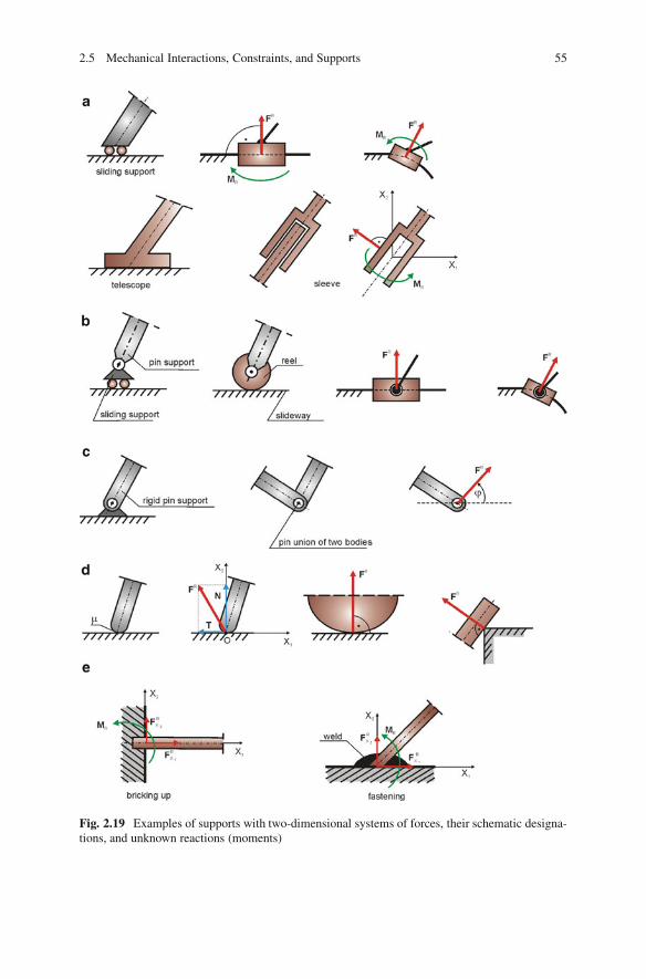
2.5 Mechanical Interactions, Constraints, and Supports 55
Fig. 2.19 Examples of supports with two-dimensional systems of forces, their schematic designa-tions, and unknown reactions (moments)
56 2 Statics
resistance to motion are used (Fig. 2.19c). Rollers are often introduced in order todecrease the motion resistance (friction) between contacting bodies, and they aretreated as massless bodies that are movable without motion resistance. In Fig. 2.19dthe contact supports with and without friction are shown. In the latter case we aredealing with one unknown, that is, the magnitude of reaction FR, since its directionis defined.
In the case of a rigidly clamped edge and restraint (Fig. 2.19e), we have threeunknowns, that is, two components of reaction and the reaction torque.
The supports discussed above that enable the point (the element) of a rigidbody in contact with a base to move in the specific (assumed in advance) direction(technical and technological manufacture of the elements of bodies in contact) wecall directional support. In this case the motion of the body can take place along astraight line or a curve.
Until now, our considerations have not taken into account the phenomenon offriction between the elements of a body in contact. The phenomenon of friction isthe subject of the next section; here it is only necessary to emphasize that in the caseof so-called fully developed friction (T D �N ) we are dealing with one unknown,and in case where T < �N (not developed friction), two unrelated forces T and Nhave to be determined.
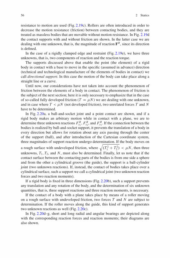
In Fig. 2.20a, a ball-and-socket joint and a point contact are shown, and if arigid body makes an arbitrary motion while in contact with a plane, we are todetermine three unknown reactions FR
x1; F R
x2, and FR
x3. If the connection between the
bodies is realized by ball-and-socket support, it prevents the translation of a body inevery direction but allows for rotation about any axis passing through the centerof the support (ball), and after introduction of the Cartesian coordinate system,three magnitudes of support reaction undergo determination. If the body moves on
a rough surface with undeveloped friction, whereq.T 21 C T 22 / < �N , then three
unknowns, T1; T2, and N , must also be determined. Finally, let us note that if thecontact surface between the contacting parts of the bodies is from one side a sphereand from the other a cylindrical groove (the guide), the support is a ball-cylinderjoint (two unknown reactions). If, instead, the contact of bodies takes place over acylindrical surface, such a support we call a cylindrical joint (two unknown reactionforces and two reaction moments).
If a rigid body is fixed in three dimensions (Fig. 2.20b), such a support preventsany translation and any rotation of the body, and the determination of six unknownquantities, that is, three support reactions and three reaction moments, is necessary.
If the contact of a body with a plane takes place by means of a roller movingon a rough surface with undeveloped friction, two forces T and N are subject todetermination. If the roller moves along the guide, this kind of support generatestwo unknown reactions as well (Fig. 2.20c).
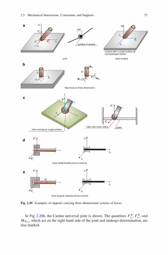
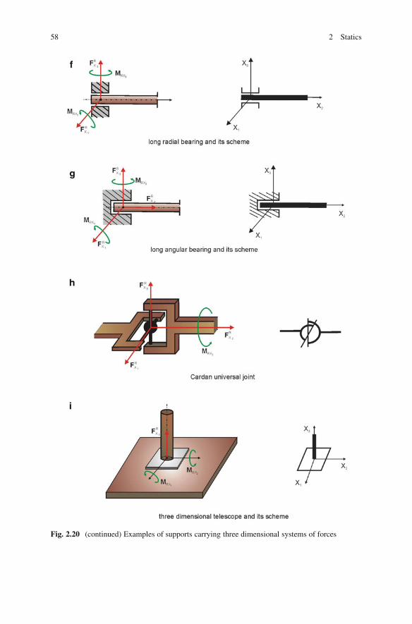
In Fig. 2.20d–g, short and long radial and angular bearings are depicted alongwith the corresponding reaction forces and reaction moments; their diagrams arealso shown.
2.5 Mechanical Interactions, Constraints, and Supports 57
Fig. 2.20 Examples of supports carrying three-dimensional systems of forces
In Fig. 2.20h, the Cardan universal joint is shown. The quantities FRx1; F R
x3, and
MRx2 , which act on the right-hand side of the joint and undergo determination, arealso marked.
58 2 Statics
Fig. 2.20 (continued) Examples of supports carrying three dimensional systems of forces
2.5 Mechanical Interactions, Constraints, and Supports 59
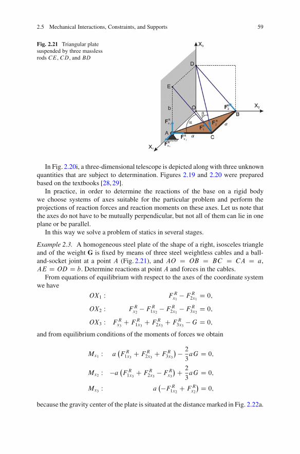
Fig. 2.21 Triangular platesuspended by three masslessrods CE , CD, and BD
In Fig. 2.20i, a three-dimensional telescope is depicted along with three unknownquantities that are subject to determination. Figures 2.19 and 2.20 were preparedbased on the textbooks [28, 29].
In practice, in order to determine the reactions of the base on a rigid bodywe choose systems of axes suitable for the particular problem and perform theprojections of reaction forces and reaction moments on these axes. Let us note thatthe axes do not have to be mutually perpendicular, but not all of them can lie in oneplane or be parallel.
In this way we solve a problem of statics in several stages.
Example 2.3. A homogeneous steel plate of the shape of a right, isosceles triangleand of the weight G is fixed by means of three steel weightless cables and a ball-and-socket joint at a point A (Fig. 2.21), and AO D OB D BC D CA D a,AE D OD D b. Determine reactions at point A and forces in the cables.
From equations of equilibrium with respect to the axes of the coordinate systemwe have
OX1 W FRx1
� FR2x1
D 0;
OX2 W FRx2
� FR1x2
� FR2x1
� FR3x2
D 0;
OX3 W F Rx3
C FR1x3
C F R2x3
C FR3x3
�G D 0;
and from equilibrium conditions of the moments of forces we obtain
Mx1 W a�F R1x3
C FR2x3
C F R3x3
�� 2
3aG D 0;
Mx2 W �a �F R1x3
C FR2x3
� FRx3
�C 2
3aG D 0;
Mx3 W a��FR
1x2C FR
x2
� D 0;
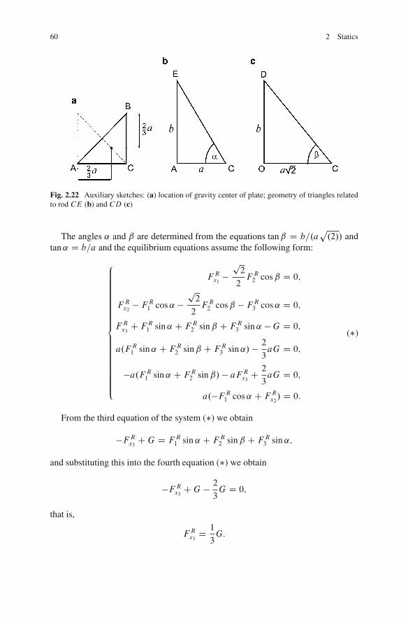
because the gravity center of the plate is situated at the distance marked in Fig. 2.22a.
60 2 Statics
Fig. 2.22 Auxiliary sketches: (a) location of gravity center of plate; geometry of triangles relatedto rod CE (b) and CD (c)
The angles ˛ and ˇ are determined from the equations tanˇ D b=.ap.2// and
tan˛ D b=a and the equilibrium equations assume the following form:
8ˆˆˆˆˆˆ<
ˆˆˆˆˆˆ:
FRx1
�p2
2F R2 cosˇ D 0;
F Rx2
� FR1 cos˛ �
p2
2F R2 cosˇ � FR
3 cos˛ D 0;
F Rx3
C FR1 sin˛ C F R
2 sinˇ C FR3 sin˛ �G D 0;
a.F R1 sin˛ C F R
2 sinˇ C FR3 sin˛/ � 2
3aG D 0;
�a.F R1 sin˛ C FR
2 sinˇ/ � aFRx3
C 2
3aG D 0;
a.�F R1 cos˛ C FR
x2/ D 0:
(�)
From the third equation of the system (�) we obtain
�F Rx3
CG D F R1 sin ˛ C FR
2 sinˇ C F R3 sin ˛;
and substituting this into the fourth equation (�) we obtain
�F Rx3
CG � 2
3G D 0;
that is,
FRx3
D 1
3G:
2.5 Mechanical Interactions, Constraints, and Supports 61
Substituting FRx3
into the fifth equation of (�) we obtain
F R1 sin ˛ C FR
2 sinˇ D 1
3G; (��)
and substituting into the third equation of (�) we have
FR3 D G
3 sin˛:
According to the sixth equation of the system (�), the second equation of (�)takes the form p
2
2F R2 cosˇ C FR
3 cos˛ D 0;
and hence after substituting the already known FR3 we obtain
F R2 D � 2G cos˛
3p2 sin ˛ cosˇ
D � 2
3p2G
cot ˛
cosˇ;
and substituting FR2 into (��) we obtain
FR1 D G
3 sin˛
�1C p
2 cot ˛ tanˇ�:
Using the sixth equation of the system (�) we have
FRx2
D G cot ˛
3
�1C p
2 cot ˛ tanˇ�;
and on the basis of the first equation of (�) we finally arrive at
FRx1
D �G3
cot ˛: ut
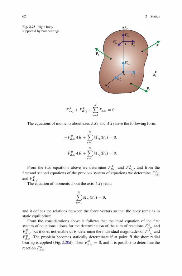
Example 2.4. Determine the reactions in support bearings of a rigid body supportedalong the vertical axis at two points A and B by means of ball bearings (Fig. 2.23)and loaded with an arbitrary force system F1; : : : ;FN .
As a result of the projection of forces on the axes of the adopted coordinatesystem we obtain
FRAx1
C F RBx1
CNX
nD1Fnx1 D 0;
F RAx2
C F RBx2
CNX
nD1Fnx2 D 0;
62 2 Statics
Fig. 2.23 Rigid bodysupported by ball bearings
FRAx3
C F RBx3
CNX
nD1Fnx3 D 0:
The equations of moments about axes AX1 and AX2 have the following form:
�FRBx2AB C
NX
nD1Mx1.Fn/ D 0;
F RBx1AB C
NX
nD1Mx2.Fn/ D 0:
From the two equations above we determine F RBx1
and F RBx2
, and from thefirst and second equations of the previous system of equations we determine F R
Ax1
and F RAx2
.The equation of moments about the axis AX3 reads
NX
nD1Mx3.Fn/ D 0;
and it defines the relations between the force vectors so that the body remains instatic equilibrium.
From the considerations above it follows that the third equation of the firstsystem of equations allows for the determination of the sum of reactions F R
Ax3and
FRBx3
, but it does not enable us to determine the individual magnitudes of FRAx3
andFRBx3
. The problem becomes statically determinate if at point B the short radialbearing is applied (Fig. 2.20d). Then FR
Bx3D 0, and it is possible to determine the
reaction FRAx3
.
2.5 Mechanical Interactions, Constraints, and Supports 63
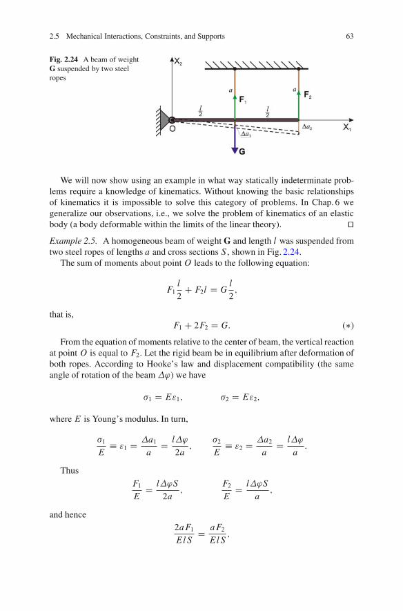
Fig. 2.24 A beam of weightG suspended by two steelropes
We will now show using an example in what way statically indeterminate prob-lems require a knowledge of kinematics. Without knowing the basic relationshipsof kinematics it is impossible to solve this category of problems. In Chap. 6 wegeneralize our observations, i.e., we solve the problem of kinematics of an elasticbody (a body deformable within the limits of the linear theory). utExample 2.5. A homogeneous beam of weight G and length l was suspended fromtwo steel ropes of lengths a and cross sections S , shown in Fig. 2.24.
The sum of moments about pointO leads to the following equation:
F1l
2C F2l D G
l
2;
that is,F1 C 2F2 D G: (�)
From the equation of moments relative to the center of beam, the vertical reactionat point O is equal to F2. Let the rigid beam be in equilibrium after deformation ofboth ropes. According to Hooke’s law and displacement compatibility (the sameangle of rotation of the beam �') we have
�1 D E"1; �2 D E"2;
where E is Young’s modulus. In turn,
�1
E� "1 D �a1
aD l�'
2a;
�2
E� "2 D �a2
aD l�'
a:
Thus
F1
ED l�'S
2a;
F2
ED l�'S
a;
and hence2aF1
ElSD aF2
ElS;
64 2 Statics
that is, 2F1 D F2. After substituting this relation into (�) we obtain successivelyF1 D 1
5G, F2 D 2
5G. ut
2.6 Reduction of a Space Force System to a Systemof Two Skew Forces
We have already mentioned the possibility of reduction of a space force systeminto a so-called equivalent system of three forces, and then to a system of two skewforces, i.e., the forces of non-intersecting lines of action.
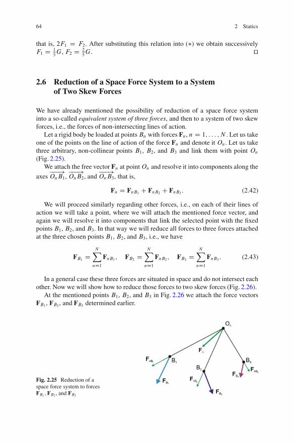
Let a rigid body be loaded at pointsBn with forces Fn, n D 1; : : : ; N . Let us takeone of the points on the line of action of the force Fn and denote it On. Let us takethree arbitrary, non-collinear points B1, B2, and B3 and link them with point On(Fig. 2.25).
We attach the free vector Fn at pointOn and resolve it into components along the
axes���!OnB1,
���!OnB2, and
���!OnB3, that is,
Fn D FnB1 C FnB2 C FnB3 : (2.42)
We will proceed similarly regarding other forces, i.e., on each of their lines ofaction we will take a point, where we will attach the mentioned force vector, andagain we will resolve it into components that link the selected point with the fixedpoints B1, B2, and B3. In that way we will reduce all forces to three forces attachedat the three chosen points B1, B2, and B3, i.e., we have
FB1 DNX
nD1FnB1 ; FB2 D
NX
nD1FnB2 ; FB3 D
NX
nD1FnB3 : (2.43)
In a general case these three forces are situated in space and do not intersect eachother. Now we will show how to reduce those forces to two skew forces (Fig. 2.26).
At the mentioned points B1, B2, and B3 in Fig. 2.26 we attach the force vectorsFB1 , FB2 , and FB3 determined earlier.
Fig. 2.25 Reduction of aspace force system to forcesFB1 ;FB2 , and FB3
2.6 Reduction to Two Skew Forces 65
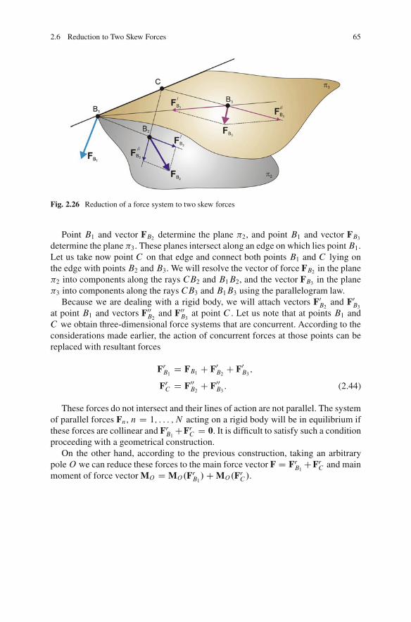
Fig. 2.26 Reduction of a force system to two skew forces
Point B1 and vector FB2 determine the plane �2, and point B1 and vector FB3determine the plane �3. These planes intersect along an edge on which lies pointB1.Let us take now point C on that edge and connect both points B1 and C lying onthe edge with points B2 and B3. We will resolve the vector of force FB2 in the plane�2 into components along the rays CB2 and B1B2, and the vector FB3 in the plane�3 into components along the rays CB3 and B1B3 using the parallelogram law.
Because we are dealing with a rigid body, we will attach vectors F0B2
and F0B3
at point B1 and vectors F00B2
and F00B3
at point C . Let us note that at points B1 andC we obtain three-dimensional force systems that are concurrent. According to theconsiderations made earlier, the action of concurrent forces at those points can bereplaced with resultant forces
FrB1 D FB1 C F0B2
C F0B3;
FrC D F00B2
C F00B3: (2.44)
These forces do not intersect and their lines of action are not parallel. The systemof parallel forces Fn, n D 1; : : : ; N acting on a rigid body will be in equilibrium ifthese forces are collinear and FrB1 CFrC D 0. It is difficult to satisfy such a conditionproceeding with a geometrical construction.
On the other hand, according to the previous construction, taking an arbitrarypoleO we can reduce these forces to the main force vector F D FrB1 CFrC and mainmoment of force vector MO D MO.FrB1/C MO.FrC /.
66 2 Statics
2.7 Reduction of a Space Force System to a Wrench
Expanding the earlier considerations concerning a plane force system, one canperform the reduction of an arbitrary space force system Fn attached at the pointsAn.x1n; x2n; x3n/, n D 1; : : : ; N to a certain arbitrarily chosen reduction poleO.x10; x20; x30/.
Let us consider the rigid body depicted in Fig. 2.11a; now the force system Fnis three-dimensional. In that figure we did not introduce the moments of force asan external load (they can be generated by the force vectors of the same lengthsand opposite senses acting in parallel directions). In this case (2.27) will remainunchanged (now S ¤ 0), but (2.29) will assume the form
Mx1 DNX
nD1
�.x2n � x20/Fx3n � .x3n � x30/Fx2n
�;
Mx2 DNX
nD1
�.x3n � x30/Fx1n � .x1n � x10/Fx3n
�;
Mx3 DNX
nD1
�.x1n � x10/Fx2n � .x2n � x20/Fx1n
�: (2.45)
In general, the magnitudes of the components of the main moment of force vectordepend on the choice of pole O , but the main force vector S does not change withthe position of pole O (it is the first invariant of reduction in statics). Often thenotion of that invariant would be introduced in the form I1 D S2x1 C S2x2 C S2x3 . Itturns out that the second invariant of reduction is the projection of the main momentof force vector M on the direction of the main force vector S, which then has theform I2 D M ı S.
Let us consider now the projection of vector M on the direction of the vector Sof the following form:
M ı S D jMjjSj cos' D MS jSj: (2.46)
Bearing in mind thatS
jSj is the unit vector, we have
MS D MS
SjSj D M ı S
jSj2 S; (2.47)
where MıSjSj2 D p is called the pitch of the wrench. Now, let us change the pole from
pointO to some other point O 0 (Fig. 2.27).
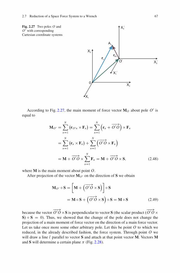
2.7 Reduction of a Space Force System to a Wrench 67
Fig. 2.27 Two poles O andO 0 with correspondingCartesian coordinate systems
According to Fig. 2.27, the main moment of force vector MO about pole O 0 isequal to
MO 0 DNX
nD1
�rO 0n � Fn
� DNX
nD1
�rn C ��!
O 0O�
� Fn
DNX
nD1
�rn � Fn
�CNX
nD1
���!O 0O � Fn
�
D M C ��!O 0O �
NX
nD1Fn D M C ��!
O 0O � S; (2.48)
where M is the main moment about pointO .After projection of the vector MO 0 on the direction of S we obtain
MO 0 ı S D�
M C���!O 0O � S
�ı S
D M ı S C���!O 0O � S
�ı S D M ı S (2.49)
because the vector��!O 0O � S is perpendicular to vector S (the scalar product .
��!O 0O �
S/ ı S D 0). Thus, we showed that the change of the pole does not change theprojection of a main moment of force vector on the direction of a main force vector.Let us take once more some other arbitrary pole. Let this be point O to which wereduced, in the already described fashion, the force system. Through point O wewill draw a line l parallel to vector S and attach at that point vector M. Vectors Mand S will determine a certain plane � (Fig. 2.28).
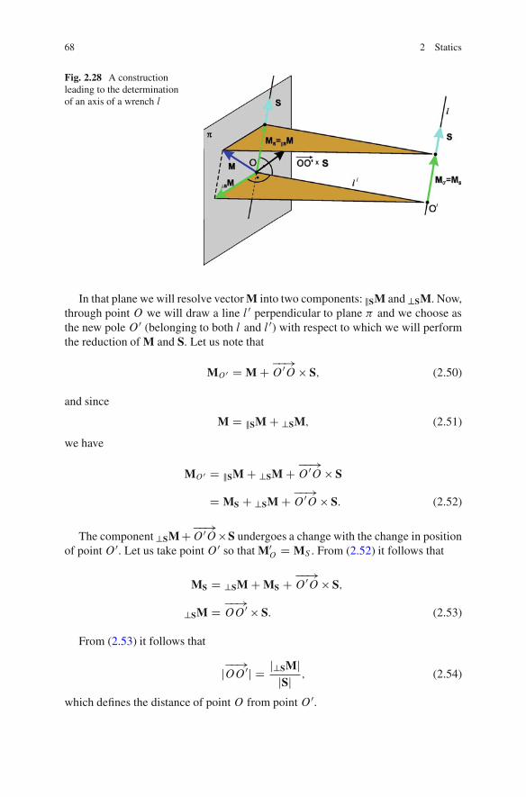
68 2 Statics
Fig. 2.28 A constructionleading to the determinationof an axis of a wrench l
In that plane we will resolve vector M into two components: kSM and ?SM. Now,through point O we will draw a line l 0 perpendicular to plane � and we choose asthe new pole O 0 (belonging to both l and l 0) with respect to which we will performthe reduction of M and S. Let us note that
MO 0 D M C ��!O 0O � S; (2.50)
and since
M D kSM C ?SM; (2.51)
we have
MO 0 D kSM C ?SM C ��!O 0O � S
D MS C ?SM C ��!O 0O � S: (2.52)
The component ?SM C��!O 0O � S undergoes a change with the change in position
of pointO 0. Let us take pointO 0 so that M0O D MS . From (2.52) it follows that
MS D ?SM C MS C ��!O 0O � S;
?SM D ��!OO 0 � S: (2.53)
From (2.53) it follows that
j��!OO 0j D j?SMj
jSj ; (2.54)
which defines the distance of point O from point O 0.
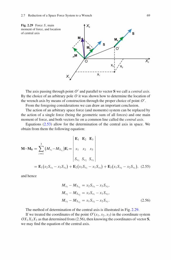
2.7 Reduction of a Space Force System to a Wrench 69
Fig. 2.29 Force S , mainmoment of force, and locationof central axis
The axis passing through pointO 0 and parallel to vector S we call a central axis.By the choice of an arbitrary pole O it was shown how to determine the location ofthe wrench axis by means of construction through the proper choice of point O 0.
From the foregoing considerations we can draw an important conclusion.The action of an arbitrary space force (and moments) system can be replaced by
the action of a single force (being the geometric sum of all forces) and one mainmoment of force, and both vectors lie on a common line called the central axis.
Equations (2.53) allow for the determination of the central axis in space. Weobtain from them the following equation:
M�MS D3X
iD1
�Mxi�MSxi
�EiD
ˇˇˇˇˇˇ
E1 E2 E3
x1 x2 x3
Sx1 Sx2 Sx3
ˇˇˇˇˇˇ
D E1�x2Sx3 � x3Sx2
�C E2�x3Sx1 � x1Sx3
�C E3�x1Sx2 � x2Sx1
�; (2.55)
and hence
Mx1 �MSx1D x2Sx3 � x3Sx2;
Mx2 �MSx2D x3Sx1 � x1Sx3;
Mx3 �MSx3D x1Sx2 � x2Sx1: (2.56)
The method of determination of the central axis is illustrated in Fig. 2.29.If we treated the coordinates of the point O 0.x1; x2; x3/ in the coordinate system
OX1X2X3 as that determined from (2.56), then knowing the coordinates of vector S,we may find the equation of the central axis.
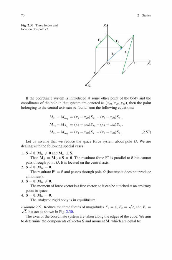
70 2 Statics
Fig. 2.30 Three forces andlocation of a pole O
If the coordinate system is introduced at some other point of the body and thecoordinates of the pole in that system are denoted as .x10; x20; x30/, then the pointbelonging to the central axis can be found from the following equations:
Mx1 �MSx1D .x2 � x20/Sx3 � .x3 � x30/Sx2;
Mx2 �MSx2D .x3 � x30/Sx1 � .x1 � x10/Sx3;
Mx3 �MSx3D .x1 � x10/Sx2 � .x2 � x20/Sx1: (2.57)
Let us assume that we reduce the space force system about pole O . We aredealing with the following special cases:
1. S ¤ 0, MO ¤ 0 and MO ? S.Then MS D MO ı S D 0. The resultant force Fr is parallel to S but cannot
pass through point O . It is located on the central axis.2. S ¤ 0, MO D 0.
The resultant Fr D S and passes through poleO (because it does not producea moment).
3. S D 0, MO ¤ 0.The moment of force vector is a free vector, so it can be attached at an arbitrary
point in space.4. S D 0, MO D 0.
The analyzed rigid body is in equilibrium.
Example 2.6. Reduce the three forces of magnitudes F1 D 1, F2 D p2, and F3 Dp
2 that act as shown in Fig. 2.30.The axes of the coordinate system are taken along the edges of the cube. We aim
to determine the components of vector S and moment M, which are equal to:
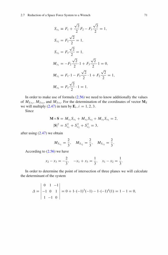
2.7 Reduction of a Space Force System to a Wrench 71
Sx1 � F1 Cp2
2F2 � F3
p2
2D 1;
Sx2 D F2
p2
2D 1;
Sx3 D F3
p2
2D 1;
Mx1 D �F2p2
2� 1C F3
p2
2� 1 D 0;
Mx2 D F1� 1� F3
p2
2� 1C F2
p2
2D 1;
Mx3 D F3
p2
2� 1 D 1:
In order to make use of formula (2.56) we need to know additionally the valuesof MSx1 , MSx2 , and MSx3 . For the determination of the coordinates of vector MS
we will multiply (2.47) in turn by Ei , i D 1; 2; 3.Since
M ı S D Mx1Sx1 CMx2Sx2 CMx3Sx3 D 2;
jSj2 D S2x1 C S2x2 C S2x3 D 3;
after using (2.47) we obtain
MSx1D 2
3; MSx2
D 2
3; MSx3
D 2
3:
According to (2.56) we have
x2 � x3 D �23; �x1 C x3 D 1
3; x1 � x2 D 1
3:
In order to determine the point of intersection of three planes we will calculatethe determinant of the system
� D
ˇˇˇˇ
0 1 �1�1 0 1
1 �1 0
ˇˇˇˇ
D 0C 1� .�1/3.�1/� 1� .�1/4.1/ D 1 � 1 D 0;
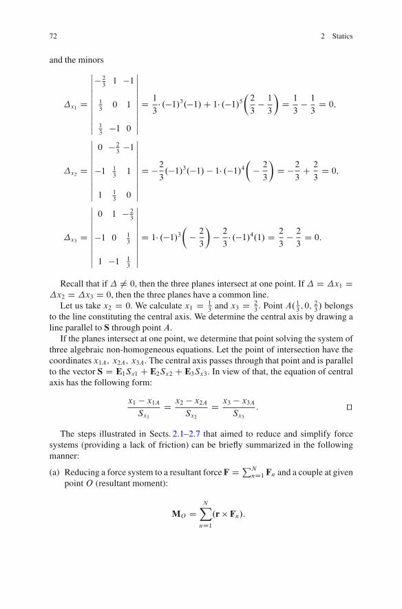
72 2 Statics
and the minors
�x1 D
ˇˇˇˇˇˇ
� 231 �1
13
0 1
13
�1 0
ˇˇˇˇˇˇ
D 1
3� .�1/3.�1/C 1� .�1/5
2
3� 1
3
�D 1
3� 1
3D 0;
�x2 D
ˇˇˇˇˇˇ
0 � 23
�1
�1 13
1
1 13
0
ˇˇˇˇˇˇ
D �23.�1/3.�1/� 1� .�1/4
� 2
3
�D �2
3C 2
3D 0;
�x3 D
ˇˇˇˇˇˇ
0 1 � 23
�1 0 13
1 �1 13
ˇˇˇˇˇˇ
D 1� .�1/3
� 2
3
�� 2
3� .�1/4.1/ D 2
3� 2
3D 0:
Recall that if � ¤ 0, then the three planes intersect at one point. If � D �x1 D�x2 D �x3 D 0, then the three planes have a common line.
Let us take x2 D 0. We calculate x1 D 13
and x3 D 23. Point A.1
3; 0; 2
3/ belongs
to the line constituting the central axis. We determine the central axis by drawing aline parallel to S through point A.
If the planes intersect at one point, we determine that point solving the system ofthree algebraic non-homogeneous equations. Let the point of intersection have thecoordinates x1A; x2A; x3A. The central axis passes through that point and is parallelto the vector S D E1Sx1 C E2Sx2 C E3Sx3. In view of that, the equation of centralaxis has the following form:
x1 � x1ASx1
D x2 � x2ASx2
D x3 � x3A
Sx3: ut
The steps illustrated in Sects. 2.1–2.7 that aimed to reduce and simplify forcesystems (providing a lack of friction) can be briefly summarized in the followingmanner:
(a) Reducing a force system to a resultant force F D PNnD1 Fn and a couple at given
pointO (resultant moment):
MO DNX
nD1.r � Fn/:
2.8 Friction 73
(b) Moving a force–couple system from point O1 to point O2, expressed by theformula
MO2 D MO1 C ���!O2O1 � F:
(c) By equivalency checking, reducing to the one point O two systems of forces,which are equivalent if the two force–couple systems are identical, i.e.,
NX
nD1Fn D
KX
kD1Fk;
NX
nD1.rn � Fn/ D
KX
kD1.Qrk � QFk/:
(d) Reducing a given force system to a single force; this takes place only ifS ? MO , i.e., when force S and couple vector MO are mutually perpendicular(which happens for concurrent coplanar and parallel forces). If position vectorr depicted from point O to any point on the line of action of the single force Fsatisfies the equation MO D r � F:
(e) Applying force and funicular polygons (Sect. 2.2).(f) Applying the three-moments theorem (Sect. 2.4).(g) Reducing a system of parallel forces (Sect. 2.4).(h) Reducing a three-dimensional force system to two skew forces (Sect. 2.6).(i) Reducing a given force system to a wrench.
In general for a three-dimensional force system (not concurrent, coplanar, orparallel) one may introduce the reduction on a basis of items (f), (h), and (i).Observe that the equivalent force system consisting of the resultant force S and thecouple vector MO are not mutually perpendicular and hence, although they cannotbe reduced to a single force, they can be reduced to a wrench since they constitutethe combination of the force S and a couple vector MS .S k MS / that lie on thewrench (case i). In other words, after reduction of a given force–couple system.S;MO/ and after determination of the pitch p D SOıMO
S2, Ms satisfies the equation
MS C r � S D MO . It allows one to find that point where the line of action of thewrench intersects a special plane (r is directed from O to that point).
2.8 Friction
The phenomenon of friction is common both in mechanics and in everyday life.Many scientific works, including monographs, cover this topic (citation is omittedhere). Also, the present author and his coworkers have published monographs onthe problems of classical friction [30–35].
74 2 Statics
In general, friction is a force that opposes a body’s motion and possesses a senseopposite to that of the velocity of the body’s relative motion. In order to ensuresliding of one surface with respect to another if both remain continuously in contact,it is necessary to act all the time on the moving body with a certain force. Thisrequirement is connected with the resistance to motion called sliding friction. This isbecause it turns out that even apparently very smooth surfaces possess irregularitiesthat cause resistance to motion. Friction is divided into static and dynamic friction.We deal with the former when we want to move one body with respect to another,e.g., remaining at rest. In the majority of cases, static friction is greater than dynamicfriction. Sliding friction depends on the condition of the contacting surfaces (i.e.,whether they are dry or lubricated), their smoothness and wear resistance abilities,and humidity and temperature.
In cases where two bodies roll with respect to one another, the friction is inverselyproportional to the radius of the object that rolls. Such friction is called rollingfriction.
Moreover, we distinguish aero and hydrodynamic friction. The former concernsthe motion of objects in gases, while the latter concerns that in liquids. For smallspeeds v of objects motion in a fluid (liquid or gas), the force of resistanceis proportional to the speed, whereas for medium (high) speeds of motion, theforce is proportional to v2 (v3). It should be emphasized that the character ofthe mentioned dependencies presents the problem rather qualitatively since thedescribed phenomenon of friction depends on the temperature, viscosity, objectshape, and fluid density. In general the friction phenomenon is not yet fullyunderstood because it is a very complex process connected with motion resistanceand accompanied by the heat generation and wear of contacting bodies. Friction canbe treated, then, also as a certain energetic process.
In most cases the kinetic energy of objects subjected to the action of frictionforces is turned into heat energy. For instance, it is widely known that objectsmoving in air such as airplanes, rockets, or spaceships are very hot, which demandsapplication of new materials of high quality and high heat resistance. Also, the rimsof wheeled vehicles heat and the striking of two firestones or rubbing of two piecesof wood leads to igniting a fire. In this case we are dealing with energy dissipation,which means that the mechanical energy (kinetic and potential) of the object is notconserved since part of it is converted into internal energy (in this case into heat).
The friction between two solid bodies, as can be seen from the precedingdescription, is a complicated physical phenomenon. Apart from the mentionedheating of bodies, often we are dealing with their electrification, changes in thesurface of the rubbing bodies, or diffusion phenomena, i.e., migration of themolecules of one body into another body.
Generally speaking, it is possible to distinguish three basic types of frictionalinteractions during the contact of two bodies: (a) sliding friction connected with thetranslational motion (no rotation) of two bodies; (b) sliding friction connected withrotational motion; (c) rolling resistance, e.g., a train wheel on a rail; and (d) slidingtorsion friction.
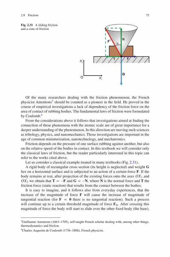
2.8 Friction 75
Fig. 2.31 A sliding frictionand a cone of friction
Of the many researchers dealing with the friction phenomenon, the Frenchphysicist Amontons3 should be counted as a pioneer in the field. He proved in thecourse of empirical investigations a lack of dependency of the friction force on thearea of contact of rubbing bodies. The fundamental laws of friction were formulatedby Coulomb.4
From the considerations above it follows that investigations aimed at finding theconnection of these phenomena with the atomic scale are of great importance for adeeper understanding of the phenomenon. In this direction are moving such sciencesas tribology, physics, and nanomechanics. Those investigations are important in theage of common miniaturization, nanotechnology, and mechatronics.
Friction depends on the pressure of one surface rubbing against another, but alsoon the relative speed of the bodies in contact. In this textbook we will consider onlythe classical laws of friction, but the reader particularly interested in this topic canrefer to the works cited above.
Let us consider a classical example treated in many textbooks (Fig. 2.31).A rigid body of rectangular cross section (its height is neglected) and weight G
lies on a horizontal surface and is subjected to an action of a certain force F. If thebody remains at rest, after projection of the existing forces onto the axes OX1 andOX2 we obtain that T D �F and G D �N, where N is the normal force and T thefriction force (static reaction) that results from the contact between the bodies.
It is easy to imagine, and it follows also from everyday experiences, that theincrease of the magnitude of force F will cause the increase of magnitude oftangential reaction (for F D 0 there is no tangential reaction). Such a processwill continue up to a certain threshold magnitude of force Fth. After crossing thismagnitude of force the body will start to slide over the other fixed body (the base),
3Guillaume Amontons (1663–1705), self-taught French scholar dealing with, among other things,thermodynamics and friction.4Charles Augustin de Coulomb (1736–1806), French physicist.
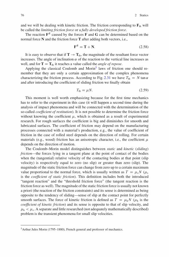
76 2 Statics
and we will be dealing with kinetic friction. The friction corresponding to Fth willbe called the limiting friction force or a fully developed friction force.
The reaction FR caused by the forces F and G can be determined based on thenormal force N and the friction force T after adding both vectors, i.e.,
FR D T C N: (2.58)
It is easy to observe that if T ! Tth, the magnitude of the resultant force vectorincreases. The angle of inclination ˛ of the reaction to the vertical line increases aswell, and for T D Tth it reaches a value called the angle of repose.
Applying the classical Coulomb and Morin5 laws of friction one should re-member that they are only a certain approximation of the complex phenomenacharacterizing the friction process. According to Fig. 2.31 we have Tth D N tan˛and after introducing the coefficient of sliding friction we finally obtain
Tth D �N: (2.59)
This moment is well worth emphasizing because for the first time mechanicshas to refer to the experiment in this case (it will happen a second time during theanalysis of impact phenomena and will be connected with the determination of theso-called coefficient of restitution). It is not possible to determine the friction forcewithout knowing the coefficient �, which is obtained as a result of experimentalresearch. For rough surfaces the coefficient is big and diminishes for smooth andlubricated surfaces. The coefficient of friction may depend on the manufacturingprocesses connected with a material’s production, e.g., the value of coefficient offriction in the case of rolled steel depends on the direction of rolling. For certainmaterials (e.g., wood) friction has an anisotropic character, i.e., the coefficient �depends on the direction of motion.
The Coulomb–Morin model distinguishes between static and kinetic (sliding)friction—the forces lying in a tangent plane at the point of contact of the bodieswhen the (tangential) relative velocity of the contacting bodies at that point (slipvelocity) is respectively equal to zero (no slip) or greater than zero (slip). Themagnitude of the static friction force can change from zero up to a certain maximumvalue proportional to the normal force, which is usually written as T D �sN (�s
is the coefficient of static friction). This definition includes both the introduced“tangent reaction” and the “threshold friction force” (the tangent reaction is thefriction force as well). The magnitude of the static friction force is usually not knowna priori (the reaction of the friction constraints) and its sense is determined as beingopposite to the tendency of sliding—sense of slip at the contact point for perfectlysmooth surfaces. The force of kinetic friction is defined as T D �kN (�k is thecoefficient of kinetic friction) and its sense is opposite to that of slip velocity, and�k < �s. A separate and little researched (not adequately mathematically described)problem is the transient phenomena for small slip velocities.
5Arthur Jules Morin (1795–1880), French general and professor of mechanics.
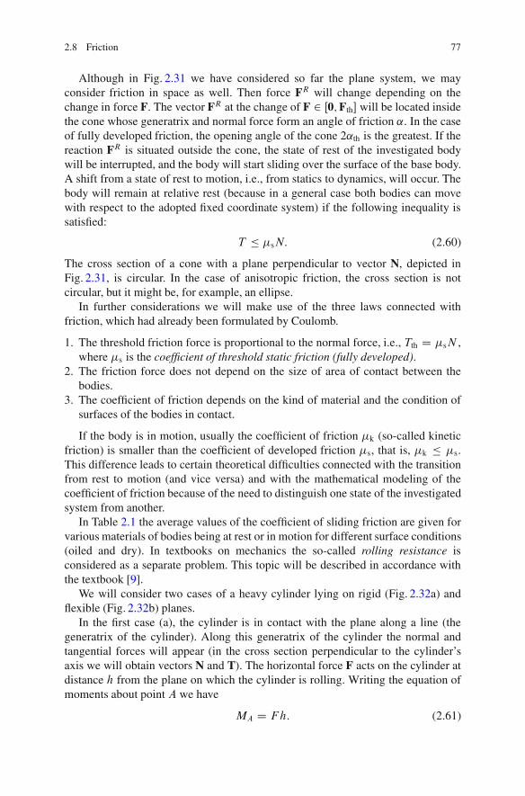
2.8 Friction 77
Although in Fig. 2.31 we have considered so far the plane system, we mayconsider friction in space as well. Then force FR will change depending on thechange in force F. The vector FR at the change of F 2 Œ0;Fth� will be located insidethe cone whose generatrix and normal force form an angle of friction ˛. In the caseof fully developed friction, the opening angle of the cone 2˛th is the greatest. If thereaction FR is situated outside the cone, the state of rest of the investigated bodywill be interrupted, and the body will start sliding over the surface of the base body.A shift from a state of rest to motion, i.e., from statics to dynamics, will occur. Thebody will remain at relative rest (because in a general case both bodies can movewith respect to the adopted fixed coordinate system) if the following inequality issatisfied:
T � �sN: (2.60)
The cross section of a cone with a plane perpendicular to vector N, depicted inFig. 2.31, is circular. In the case of anisotropic friction, the cross section is notcircular, but it might be, for example, an ellipse.
In further considerations we will make use of the three laws connected withfriction, which had already been formulated by Coulomb.
1. The threshold friction force is proportional to the normal force, i.e., Tth D �sN ,where �s is the coefficient of threshold static friction (fully developed).
2. The friction force does not depend on the size of area of contact between thebodies.
3. The coefficient of friction depends on the kind of material and the condition ofsurfaces of the bodies in contact.
If the body is in motion, usually the coefficient of friction �k (so-called kineticfriction) is smaller than the coefficient of developed friction �s, that is, �k � �s.This difference leads to certain theoretical difficulties connected with the transitionfrom rest to motion (and vice versa) and with the mathematical modeling of thecoefficient of friction because of the need to distinguish one state of the investigatedsystem from another.
In Table 2.1 the average values of the coefficient of sliding friction are given forvarious materials of bodies being at rest or in motion for different surface conditions(oiled and dry). In textbooks on mechanics the so-called rolling resistance isconsidered as a separate problem. This topic will be described in accordance withthe textbook [9].
We will consider two cases of a heavy cylinder lying on rigid (Fig. 2.32a) andflexible (Fig. 2.32b) planes.
In the first case (a), the cylinder is in contact with the plane along a line (thegeneratrix of the cylinder). Along this generatrix of the cylinder the normal andtangential forces will appear (in the cross section perpendicular to the cylinder’saxis we will obtain vectors N and T). The horizontal force F acts on the cylinder atdistance h from the plane on which the cylinder is rolling. Writing the equation ofmoments about point A we have
MA D Fh: (2.61)
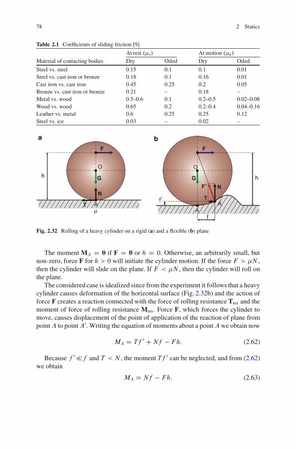
78 2 Statics
Table 2.1 Coefficients of sliding friction [9]
At rest .�s/ At motion .�k/
Material of contacting bodies Dry Oiled Dry Oiled
Steel vs. steel 0.15 0.1 0.1 0.01Steel vs. cast iron or bronze 0.18 0.1 0.16 0.01Cast iron vs. cast iron 0.45 0.25 0.2 0.05Bronze vs. cast iron or bronze 0.21 – 0.18 –Metal vs. wood 0.5–0.6 0.1 0.2–0.5 0.02–0.08Wood vs. wood 0.65 0.2 0.2–0.4 0.04–0.16Leather vs. metal 0.6 0.25 0.25 0.12Steel vs. ice 0.03 – 0.02 –
Fig. 2.32 Rolling of a heavy cylinder on a rigid (a) and a flexible (b) plane
The moment MA D 0 if F D 0 or h D 0. Otherwise, an arbitrarily small, butnon-zero, force F for h > 0 will initiate the cylinder motion. If the force F > �N ,then the cylinder will slide on the plane. If F < �N , then the cylinder will roll onthe plane.
The considered case is idealized since from the experiment it follows that a heavycylinder causes deformation of the horizontal surface (Fig. 2.32b) and the action offorce F creates a reaction connected with the force of rolling resistance Tres and themoment of force of rolling resistance Mres. Force F, which forces the cylinder tomove, causes displacement of the point of application of the reaction of plane frompointA to pointA0. Writing the equation of moments about a pointAwe obtain now
MA D Tf 0 CNf � Fh: (2.62)
Because f 0�f and T < N , the moment Tf 0 can be neglected, and from (2.62)we obtain
MA D Nf � Fh: (2.63)

2.8 Friction 79
Table 2.2 Rolling resistance coefficients [9]
Cylinder Basis f .10�2 m/
Cast iron Cast iron 0.005Steel Steel rail 0.005Wooden Wood 0.8Roller bearings and balls
(hardened and ground)Hardened and
ground steel0.0005–0.001
The motion will start when the moment Fh overcomes the momentNf D Mres,called a moment of rolling resistance. The quantity f we call a coefficient of rollingresistance or an arm of rolling resistance. Let us note that, as distinct from thedimensionless coefficient �, the quantity f possesses a dimension of length andcharacterizes the maximum distance at which the point of application of reactioncan move preserving the state of rest of the body, i.e., when Fh D Nf . Severalaverage values of the coefficient of rolling resistance f for various materials of thecylinder and ground are given in Table 2.2.
The third case of the classical division of friction, i.e., rotational friction, remainsto be described. In the case of sliding friction the problem can be reduced to thepoint of contact. If, however, to one (or both) of the contacting bodies we applya moment of force, the assumption of their contact only at the point is not valid.The moment of force is carried by the moment of friction forces that must occurover a certain (although very small) area. Thus, the moment of force is balancednot by a single force but by a couple of forces. After overcoming the momentof rotational friction, the moment of force will cause rotation of the body onwhich it acts (on the assumption that the other body remains fixed) about an axisperpendicular to the surface of contact of the bodies. The threshold magnitude ofthe moment of rotational friction is usually assumed to be proportional to the forceN (which is the force compressing the bodies, normal to the surface of contact), andthat threshold magnitude equals MF D �0N , where now �0 denotes a rotationalfriction coefficient, and this time the coefficient �0 possesses a dimension of length.The problem is relatively complex since the moment of friction force depends onthe normal stress in the area of contact (area size greater than zero) distribution,which must be uniform over the mentioned area. Additionally, the rotational frictioncoefficient depends on the coefficient of forward sliding friction because it is causedby the normal force N. For example, from the theoretical considerations concerningthe contact problem of the cylinder of radius r making contact with the fixed surfaceover the area �r2, the coefficient of rotational friction �0 D 0:25�r�, where �denotes the sliding friction.
Let us consider a classical case of a rigid body having the shape of a rectangularprism (Fig. 2.33), but in the present case we assume that the dimensions of its crosssection with a vertical plane, i.e., width 2b and height 2h of rectangle, are known.We will also assume that its geometrical center coincides with the center of mass(point C ) and that at point C the gravity force G and horizontal force F are applied(Fig. 2.33).
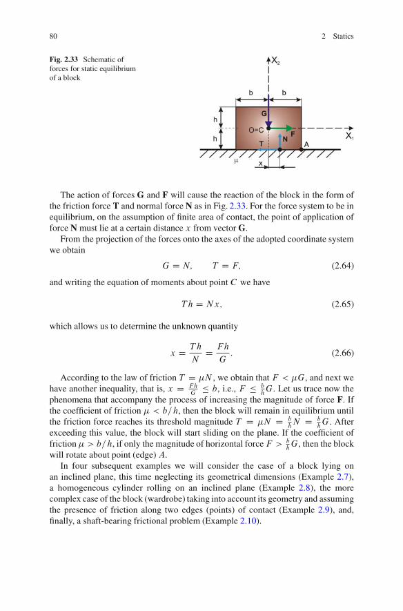
80 2 Statics
Fig. 2.33 Schematic offorces for static equilibriumof a block
The action of forces G and F will cause the reaction of the block in the form ofthe friction force T and normal force N as in Fig. 2.33. For the force system to be inequilibrium, on the assumption of finite area of contact, the point of application offorce N must lie at a certain distance x from vector G.
From the projection of the forces onto the axes of the adopted coordinate systemwe obtain
G D N; T D F; (2.64)
and writing the equation of moments about point C we have
T h D Nx; (2.65)
which allows us to determine the unknown quantity
x D T h
ND Fh
G: (2.66)
According to the law of friction T D �N , we obtain that F < �G, and next wehave another inequality, that is, x D Fh
G� b, i.e., F � b
hG. Let us trace now the
phenomena that accompany the process of increasing the magnitude of force F. Ifthe coefficient of friction � < b=h, then the block will remain in equilibrium untilthe friction force reaches its threshold magnitude T D �N D b
hN D b
hG. After
exceeding this value, the block will start sliding on the plane. If the coefficient offriction� > b=h, if only the magnitude of horizontal forceF > b
hG, then the block
will rotate about point (edge) A.In four subsequent examples we will consider the case of a block lying on
an inclined plane, this time neglecting its geometrical dimensions (Example 2.7),a homogeneous cylinder rolling on an inclined plane (Example 2.8), the morecomplex case of the block (wardrobe) taking into account its geometry and assumingthe presence of friction along two edges (points) of contact (Example 2.9), and,finally, a shaft-bearing frictional problem (Example 2.10).
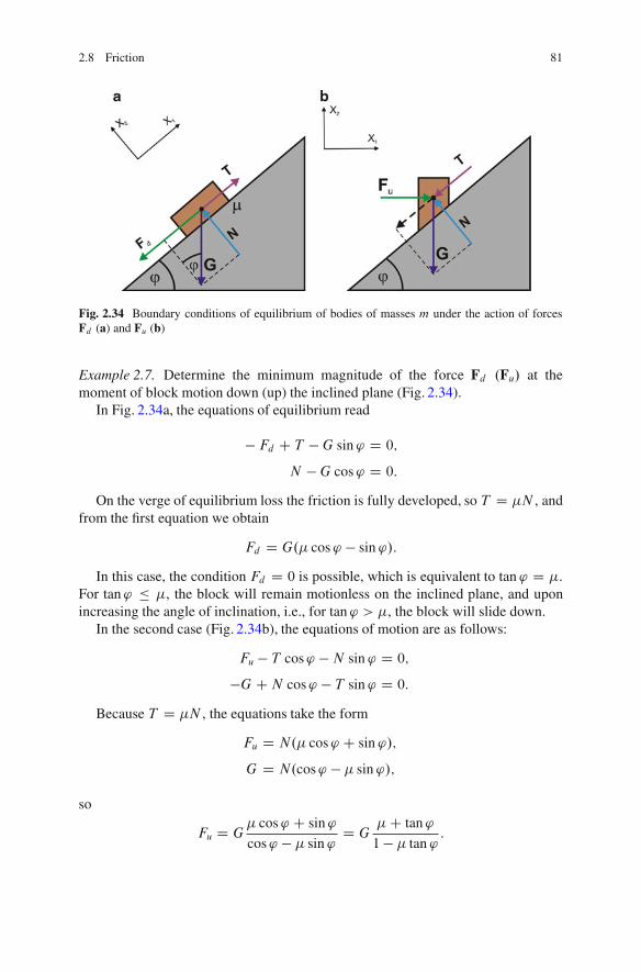
2.8 Friction 81
Fig. 2.34 Boundary conditions of equilibrium of bodies of masses m under the action of forcesFd (a) and Fu (b)
Example 2.7. Determine the minimum magnitude of the force Fd .Fu/ at themoment of block motion down (up) the inclined plane (Fig. 2.34).
In Fig. 2.34a, the equations of equilibrium read
� Fd C T �G sin ' D 0;
N �G cos' D 0:
On the verge of equilibrium loss the friction is fully developed, so T D �N , andfrom the first equation we obtain
Fd D G.� cos' � sin '/:
In this case, the condition Fd D 0 is possible, which is equivalent to tan ' D �.For tan' � �, the block will remain motionless on the inclined plane, and uponincreasing the angle of inclination, i.e., for tan' > �, the block will slide down.
In the second case (Fig. 2.34b), the equations of motion are as follows:
Fu � T cos' �N sin ' D 0;
�G CN cos' � T sin ' D 0:
Because T D �N , the equations take the form
Fu D N.� cos' C sin '/;
G D N.cos' � � sin '/;
so
Fu D G� cos' C sin'
cos' � � sin 'D G
�C tan'
1� � tan ':
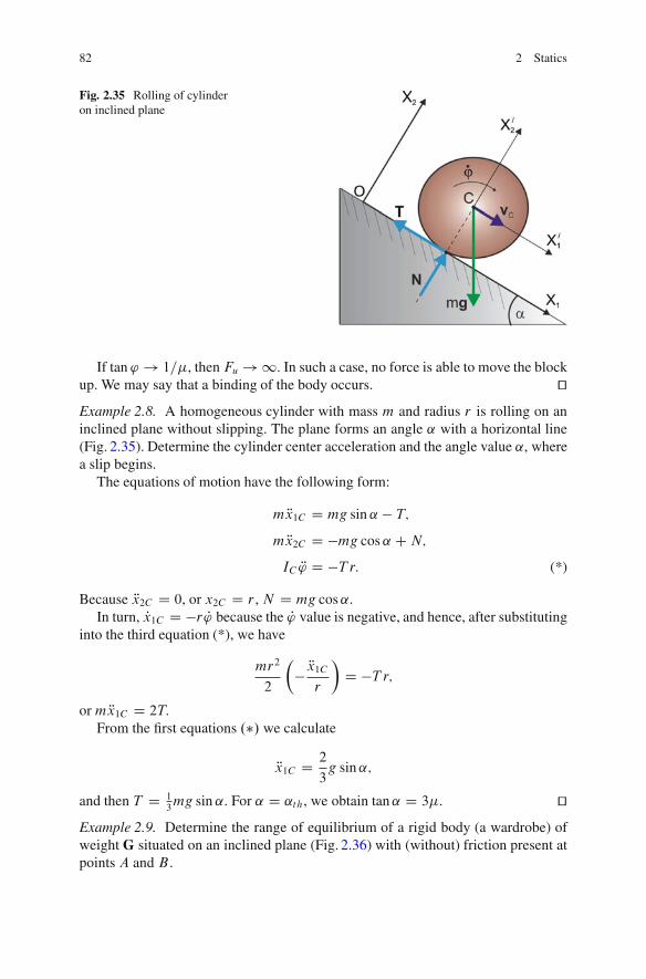
82 2 Statics
Fig. 2.35 Rolling of cylinderon inclined plane
If tan ' ! 1=�, then Fu ! 1. In such a case, no force is able to move the blockup. We may say that a binding of the body occurs. utExample 2.8. A homogeneous cylinder with mass m and radius r is rolling on aninclined plane without slipping. The plane forms an angle ˛ with a horizontal line(Fig. 2.35). Determine the cylinder center acceleration and the angle value ˛, wherea slip begins.
The equations of motion have the following form:
m Rx1C D mg sin ˛ � T;
m Rx2C D �mg cos˛ CN;
IC R' D �T r: (*)
Because Rx2C D 0, or x2C D r , N D mg cos˛.In turn, Px1C D �r P' because the P' value is negative, and hence, after substituting
into the third equation (*), we have
mr2
2
� Rx1Cr
�D �T r;
or m Rx1C D 2T:
From the first equations .�/ we calculate
Rx1C D 2
3g sin˛;
and then T D 13mg sin ˛. For ˛ D ˛th, we obtain tan˛ D 3�. ut
Example 2.9. Determine the range of equilibrium of a rigid body (a wardrobe) ofweight G situated on an inclined plane (Fig. 2.36) with (without) friction present atpoints A and B .
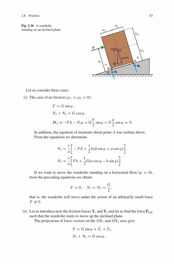
2.8 Friction 83
Fig. 2.36 A wardrobestanding on an inclined plane
Let us consider three cases.
(i) The case of no friction (�1 D �2 D 0):
F D G sin ';
N1 CN2 D G cos';
MA � �Fh �N1aCGb
2sin' CG
a
2cos' D 0:
In addition, the equation of moments about point A was written above.From the equations we determine
N1 D 1
a
�� FhC 1
2G.b sin' C a cos'/
;
N2 D 1
a
�FhC 1
2G.a cos' � b sin'/
:
If we want to move the wardrobe standing on a horizontal floor (' D 0),from the preceding equations we obtain
F D 0; N1 D N2 D G
2;
that is, the wardrobe will move under the action of an arbitrarily small forceF ¤ 0.
(ii) Let us introduce now the friction forces T1 and T2 and let us find the force Fmin
such that the wardrobe starts to move up the inclined plane.The projections of force vectors on the OX1 andOX2 axes give
F D G sin' C T1 C T2;
N1 CN2 D G cos':
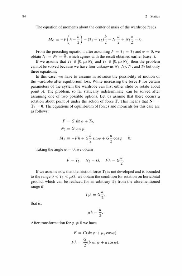
84 2 Statics
The equation of moments about the center of mass of the wardrobe reads
MO � �Fh � b
2
�� .T1 C T2/
b
2�N1
a
2CN2
a
2D 0:
From the preceding equation, after assuming F D T1 D T2 and ' D 0, weobtain N1 D N2 D G
2, which agrees with the result obtained earlier (case i).
If we assume that T1 2 Œ0; �1N1� and T2 2 Œ0; �2N2�, then the problemcannot be solved because we have four unknownsN1;N2; T1, and T2 but onlythree equations.
In this case, we have to assume in advance the possibility of motion ofthe wardrobe after equilibrium loss. While increasing the force F for certainparameters of the system the wardrobe can first either slide or rotate aboutpoint A. The problem, so far statically indeterminate, can be solved afterassuming one of two possible options. Let us assume that there occurs arotation about point A under the action of force F. This means that N1 DT1 D 0. The equations of equilibrium of forces and moments for this case areas follows:
F D G sin ' C T2;
N2 D G cos';
MA � �FhCGb
2sin' CG
a
2cos' D 0:
Taking the angle ' D 0, we obtain
F D T2; N2 D G; F h D Ga
2:
If we assume now that the friction force T2 is not developed and is boundedto the range 0 < T2 < �G, we obtain the condition for rotation on horizontalground, which can be realized for an arbitrary T2 from the aforementionedrange if
T2h D Ga
2;
that is,
�h D a
2:
After transformation for ' ¤ 0 we have
F D G.sin' C �2 cos'/;
F h D G
2.b sin ' C a cos'/;
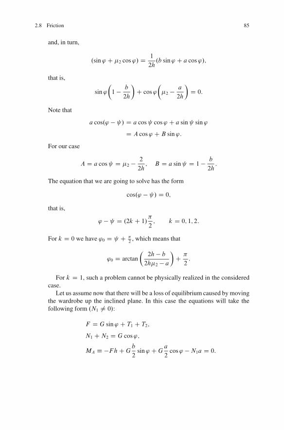
2.8 Friction 85
and, in turn,
.sin ' C �2 cos'/ D 1
2h.b sin' C a cos'/;
that is,
sin '
1 � b
2h
�C cos'
�2 � a
2h
�D 0:
Note that
a cos.' � / D a cos cos' C a sin sin '
D A cos' C B sin ':
For our case
A D a cos D �2 � 2
2h; B D a sin D 1 � b
2h:
The equation that we are going to solve has the form
cos.' � / D 0;
that is,
' � D .2k C 1/�
2; k D 0; 1; 2:
For k D 0 we have '0 D C �2
, which means that
'0 D arctan
2h� b
2h�2 � a
�C �
2:
For k D 1, such a problem cannot be physically realized in the consideredcase.
Let us assume now that there will be a loss of equilibrium caused by movingthe wardrobe up the inclined plane. In this case the equations will take thefollowing form .N1 ¤ 0/:
F D G sin ' C T1 C T2;
N1 CN2 D G cos';
MA � �FhCGb
2sin ' CG
a
2cos' �N1a D 0:
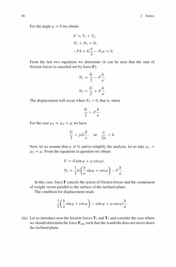
86 2 Statics
For the angle ' D 0 we obtain
F D T1 C T2;
N1 CN2 D G;
�FhCGa
2�N1a D 0:
From the last two equations we determine (it can be seen that the sum offriction forces is canceled out by force F):
N1 D G
2� F
h
a;
N2 D G
2C F
h
a:
The displacement will occur when N1 > 0, that is, when
G
2> F
h
a:
For the case �1 D �2 D � we have
G
2> �G
h
a; or
a
2�> h:
Now, let us assume that ' ¤ 0, and to simplify the analysis, let us take �1 D�2 D �. From the equations in question we obtain
F D G.sin ' C � cos'/;
N1 D 1
2G
b
asin ' C cos'
�� F h
a:
In this case, force F cancels the action of friction forces and the componentof weight vector parallel to the surface of the inclined plane.
The condition for displacement reads
1
2
b
asin ' C cos'
�> .sin ' C � cos'/
h
a:
(iii) Let us introduce now the friction forces T1 and T2 and consider the case wherewe should determine the force Fmin such that the wardrobe does not move downthe inclined plane.
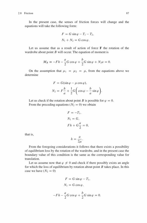
2.8 Friction 87
In the present case, the senses of friction forces will change and theequations will take the following form:
F D G sin ' � T1 � T2;N1 CN2 D G cos':
Let us assume that as a result of action of force F the rotation of thewardrobe about point B will occur. The equation of moment is
MB � �Fh � a
2G cos' C b
2G sin ' CN2a D 0:
On the assumption that �1 D �2 D �, from the equations above wedetermine
F D G.sin' � � cos'/;
N2 D Fh
aC 1
2G
cos' � b
asin '
�:
Let us check if the rotation about point B is possible for ' D 0.From the preceding equations (N2 D 0) we obtain
F D �T1;N1 D G;
FhCGa
2D 0;
that is,
h D a
2�:
From the foregoing considerations it follows that there exists a possibilityof equilibrium loss by the rotation of the wardrobe, and in the present case theboundary value of this condition is the same as the corresponding value fortranslation.
Let us assume now that ' ¤ 0 and check if there possibly exists an anglefor which the loss of equilibrium by rotation about point B takes place. In thiscase we have (N2 D 0)
F D G sin ' � T1;
N1 D G cos';
�Fh� a
2G cos' C b
2G sin' D 0:
88 2 Statics
Then we have
h.sin ' � � cos'/ D 1
2.�a cos' C b sin '/;
and after transformations we obtain
� hC b
2
�sin' C
h� � a
2
�cos' D 0:
Let us assume now that the equilibrium loss will occur by the motion ofthe wardrobe down the inclined plane, so the loss of equilibrium will resultin sliding. The condition of the motion is N2 0 and in the boundary caseN2 D 0. This condition is identical with the one for the rotation about pointB .
Let us note that the current example allows for the analysis of two special cases.For ' D 0 we are dealing with the problem of equilibrium loss of the wardrobesituated on a horizontal surface (already presented). Let us assume now that a Db D h D 0, that is, we will be considering a particle of mass m situated on theinclined plane .N1 C N2 D N/.
From the considerations conducted for case (i) we obtain
F D mg sin ';
N D mg cos':
This means that for the particle to remain at rest on the inclined plane one shouldapply to it force F of magnitudemg sin'.
In case (ii) we have
F �min D G.sin' C � cos'/;
whereas in case (iii) we have
Fmin D G.sin' � � cos'/:
Let us note that for the forces within the range F 2 ŒFmin; F�min� the particle
remains in equilibrium. Range ŒFmin; F�min� we will call the range of equilibrium
loading. utExample 2.10. Determine the angle of friction ' and so-called circle of friction ofradius r during contact of the shaft journal of radius R and the bearing shell onthe assumption that the radius of the bearing shell is slightly larger than R and wasomitted in Fig. 2.37.
Let us assume that the shaft journal is loaded with a couple of moment M and aforce F. The action of the moment causes the displacement of the point of contactA between the journal and the bearing shell upward, i.e., we are dealing with thephenomenon of shaft climbing.
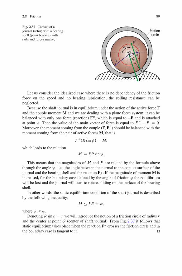
2.8 Friction 89
Fig. 2.37 Contact of ajournal (rotor) with a bearingshell (plain bearing) withradii and forces marked
Let us consider the idealized case where there is no dependency of the frictionforce on the speed and no bearing lubrication; the rolling resistance can beneglected.
Because the shaft journal is in equilibrium under the action of the active force Fand the couple moment M and we are dealing with a plane force system, it can bebalanced with only one force (reaction) FR, which is equal to �F and is attachedat point A. Then the value of the main vector of force is equal to F R � F D 0.Moreover, the moment coming from the couple (F;FR) should be balanced with themoment coming from the pair of active forces M, that is
F R.R sin / D M;
which leads to the relation
M D FR sin :
This means that the magnitudes of M and F are related by the formula abovethrough the angle , i.e., the angle between the normal to the contact surface of thejournal and the bearing shell and the reaction FR. If the magnitude of moment M isincreased, for the boundary case defined by the angle of friction ' the equilibriumwill be lost and the journal will start to rotate, sliding on the surface of the bearingshell.
In other words, the static equilibrium condition of the shaft journal is describedby the following inequality:
M � FR sin ';
where � '.DenotingR sin' D r we will introduce the notion of a friction circle of radius r
and the center at point O (center of shaft journal). From Fig. 2.37 it follows thatstatic equilibrium takes place when the reaction FR crosses the friction circle and inthe boundary case is tangent to it. ut
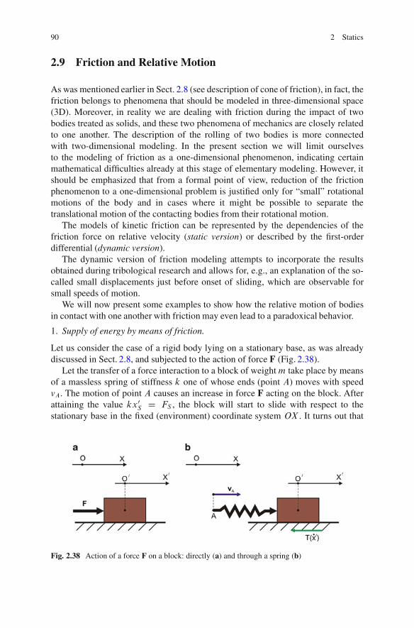
90 2 Statics
2.9 Friction and Relative Motion
As was mentioned earlier in Sect. 2.8 (see description of cone of friction), in fact, thefriction belongs to phenomena that should be modeled in three-dimensional space(3D). Moreover, in reality we are dealing with friction during the impact of twobodies treated as solids, and these two phenomena of mechanics are closely relatedto one another. The description of the rolling of two bodies is more connectedwith two-dimensional modeling. In the present section we will limit ourselvesto the modeling of friction as a one-dimensional phenomenon, indicating certainmathematical difficulties already at this stage of elementary modeling. However, itshould be emphasized that from a formal point of view, reduction of the frictionphenomenon to a one-dimensional problem is justified only for “small” rotationalmotions of the body and in cases where it might be possible to separate thetranslational motion of the contacting bodies from their rotational motion.
The models of kinetic friction can be represented by the dependencies of thefriction force on relative velocity (static version) or described by the first-orderdifferential (dynamic version).
The dynamic version of friction modeling attempts to incorporate the resultsobtained during tribological research and allows for, e.g., an explanation of the so-called small displacements just before onset of sliding, which are observable forsmall speeds of motion.
We will now present some examples to show how the relative motion of bodiesin contact with one another with friction may even lead to a paradoxical behavior.
1. Supply of energy by means of friction.
Let us consider the case of a rigid body lying on a stationary base, as was alreadydiscussed in Sect. 2.8, and subjected to the action of force F (Fig. 2.38).
Let the transfer of a force interaction to a block of weightm take place by meansof a massless spring of stiffness k one of whose ends (point A) moves with speedvA. The motion of point A causes an increase in force F acting on the block. Afterattaining the value kx0
S D FS , the block will start to slide with respect to thestationary base in the fixed (environment) coordinate system OX . It turns out that
Fig. 2.38 Action of a force F on a block: directly (a) and through a spring (b)
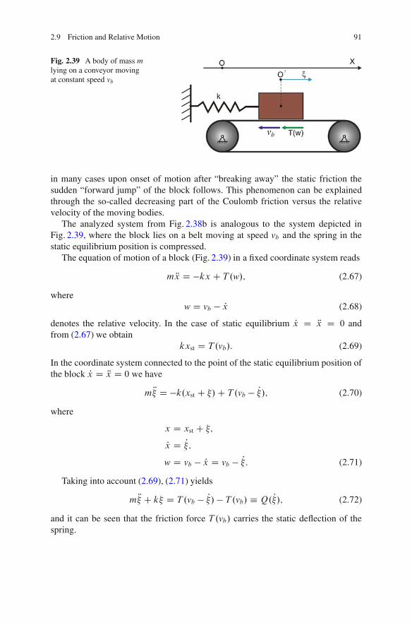
2.9 Friction and Relative Motion 91
Fig. 2.39 A body of mass mlying on a conveyor movingat constant speed vb
in many cases upon onset of motion after “breaking away” the static friction thesudden “forward jump” of the block follows. This phenomenon can be explainedthrough the so-called decreasing part of the Coulomb friction versus the relativevelocity of the moving bodies.
The analyzed system from Fig. 2.38b is analogous to the system depicted inFig. 2.39, where the block lies on a belt moving at speed vb and the spring in thestatic equilibrium position is compressed.
The equation of motion of a block (Fig. 2.39) in a fixed coordinate system reads
m Rx D �kx C T .w/; (2.67)
wherew D vb � Px (2.68)
denotes the relative velocity. In the case of static equilibrium Px D Rx D 0 andfrom (2.67) we obtain
kxst D T .vb/: (2.69)
In the coordinate system connected to the point of the static equilibrium position ofthe block Px D Rx D 0 we have
m R� D �k.xst C �/C T .vb � P�/; (2.70)
where
x D xst C �;
Px D P�;w D vb � Px D vb � P�: (2.71)
Taking into account (2.69), (2.71) yields
m R� C k� D T .vb � P�/� T .vb/ � Q. P�/; (2.72)
and it can be seen that the friction force T .vb/ carries the static deflection of thespring.
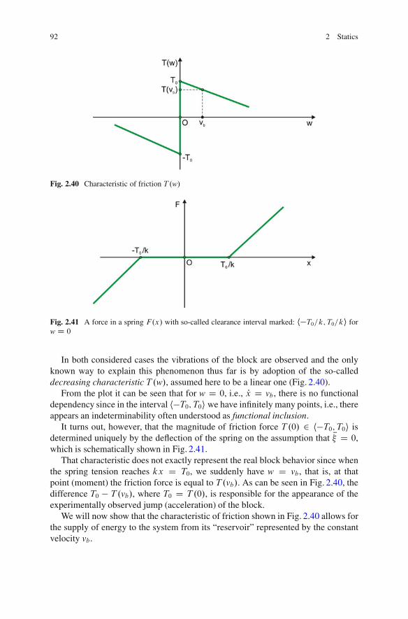
92 2 Statics
Fig. 2.40 Characteristic of friction T .w/
Fig. 2.41 A force in a spring F.x/ with so-called clearance interval marked: h�T0=k; T0=ki forw D 0
In both considered cases the vibrations of the block are observed and the onlyknown way to explain this phenomenon thus far is by adoption of the so-calleddecreasing characteristic T .w/, assumed here to be a linear one (Fig. 2.40).
From the plot it can be seen that for w D 0, i.e., Px D vb , there is no functionaldependency since in the interval h�T0; T0i we have infinitely many points, i.e., thereappears an indeterminability often understood as functional inclusion.
It turns out, however, that the magnitude of friction force T .0/ 2 h�T0; T0i isdetermined uniquely by the deflection of the spring on the assumption that R� D 0,which is schematically shown in Fig. 2.41.
That characteristic does not exactly represent the real block behavior since whenthe spring tension reaches kx D T0, we suddenly have w D vb , that is, at thatpoint (moment) the friction force is equal to T .vb/. As can be seen in Fig. 2.40, thedifference T0 � T .vb/, where T0 D T .0/, is responsible for the appearance of theexperimentally observed jump (acceleration) of the block.
We will now show that the characteristic of friction shown in Fig. 2.40 allows forthe supply of energy to the system from its “reservoir” represented by the constantvelocity vb .
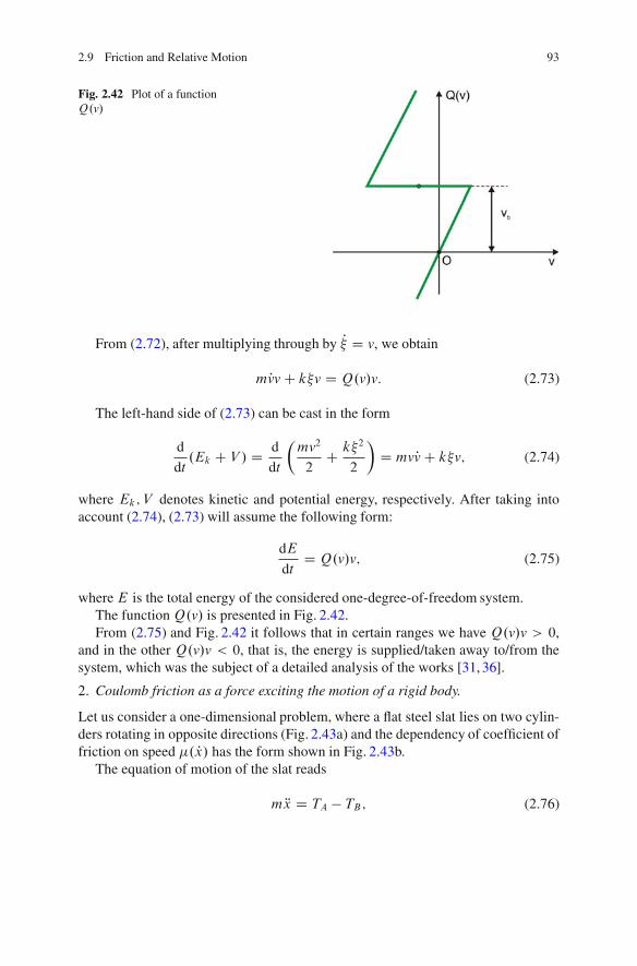
2.9 Friction and Relative Motion 93
Fig. 2.42 Plot of a functionQ.v/
From (2.72), after multiplying through by P� D v, we obtain
mPvv C k�v D Q.v/v: (2.73)
The left-hand side of (2.73) can be cast in the form
d
dt.Ek C V / D d
dt
mv2
2C k�2
2
�D mvPv C k�v; (2.74)
where Ek; V denotes kinetic and potential energy, respectively. After taking intoaccount (2.74), (2.73) will assume the following form:
dE
dtD Q.v/v; (2.75)
where E is the total energy of the considered one-degree-of-freedom system.The functionQ.v/ is presented in Fig. 2.42.From (2.75) and Fig. 2.42 it follows that in certain ranges we have Q.v/v > 0,
and in the other Q.v/v < 0, that is, the energy is supplied/taken away to/from thesystem, which was the subject of a detailed analysis of the works [31, 36].
2. Coulomb friction as a force exciting the motion of a rigid body.
Let us consider a one-dimensional problem, where a flat steel slat lies on two cylin-ders rotating in opposite directions (Fig. 2.43a) and the dependency of coefficient offriction on speed �. Px/ has the form shown in Fig. 2.43b.
The equation of motion of the slat reads
m Rx D TA � TB; (2.76)
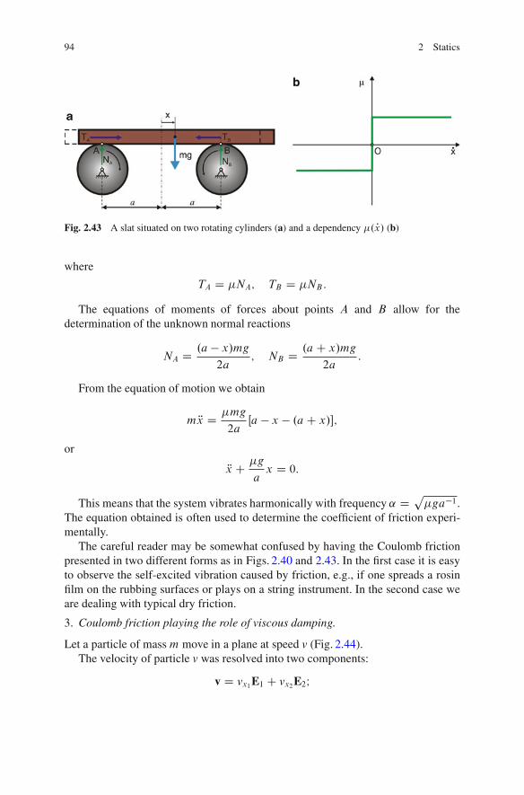
94 2 Statics
Fig. 2.43 A slat situated on two rotating cylinders (a) and a dependency �. Px/ (b)
where
TA D �NA; TB D �NB:
The equations of moments of forces about points A and B allow for thedetermination of the unknown normal reactions
NA D .a � x/mg
2a; NB D .a C x/mg
2a:
From the equation of motion we obtain
m Rx D �mg
2aŒa � x � .aC x/�;
or
Rx C �g
ax D 0:
This means that the system vibrates harmonically with frequency ˛ D p�ga�1.
The equation obtained is often used to determine the coefficient of friction experi-mentally.
The careful reader may be somewhat confused by having the Coulomb frictionpresented in two different forms as in Figs. 2.40 and 2.43. In the first case it is easyto observe the self-excited vibration caused by friction, e.g., if one spreads a rosinfilm on the rubbing surfaces or plays on a string instrument. In the second case weare dealing with typical dry friction.
3. Coulomb friction playing the role of viscous damping.
Let a particle of mass m move in a plane at speed v (Fig. 2.44).The velocity of particle v was resolved into two components:
v D vx1E1 C vx2E2I
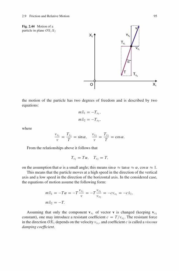
2.9 Friction and Relative Motion 95
Fig. 2.44 Motion of aparticle in plane OX1X2
the motion of the particle has two degrees of freedom and is described by twoequations:
m Rx1 D �Tx1;m Rx2 D �Tx2;
wherevx1v
D Tx1T
D sin˛;vx2v
D Tx2T
D cos˛:
From the relationships above it follows that
Tx1 D T˛; Tx2 D T;
on the assumption that ˛ is a small angle; this means sin ˛ tan˛ ˛, cos˛ 1.This means that the particle moves at a high speed in the direction of the vertical
axis and a low speed in the direction of the horizontal axis. In the considered case,the equations of motion assume the following form:
m Rx1 D �T˛ D �T vx1v
D �T vx1vx2
D �cvx1 D �c Px1;
m Rx2 D �T:
Assuming that only the component vx1 of vector v is changed (keeping vx2constant), one may introduce a resistant coefficient c D T=vx2 . The resistant forcein the directionOX1 depends on the velocity vx1 , and coefficient c is called a viscousdamping coefficient.
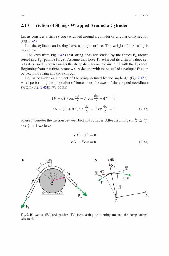
96 2 Statics
2.10 Friction of Strings Wrapped Around a Cylinder
Let us consider a string (rope) wrapped around a cylinder of circular cross section(Fig. 2.45).
Let the cylinder and string have a rough surface. The weight of the string isnegligible.
It follows from Fig. 2.45a that string ends are loaded by the forces Fa (activeforce) and Fp (passive force). Assume that force Fa achieved its critical value, i.e.,infinitely small increase yields the string displacement coinciding with the Fa sense.Beginning from that time instant we are dealing with the so-called developed frictionbetween the string and the cylinder.
Let us consider an element of the string defined by the angle d' (Fig. 2.45a).After performing the projection of forces onto the axes of the adopted coordinatesystem (Fig. 2.45b), we obtain
.F C dF / cosd'
2� F cos
d'
2� dT D 0;
dN � .F C dF / sind'
2� F sin
d'
2D 0; (2.77)
where T denotes the friction between belt and cylinder. After assuming sin d'2
Š d'2
,
cos d'2
Š 1 we have
dF � dT D 0;
dN � F d' D 0: (2.78)
Fig. 2.45 Active (Fa) and passive (Fp) force acting on a string (a) and the computationalscheme (b)
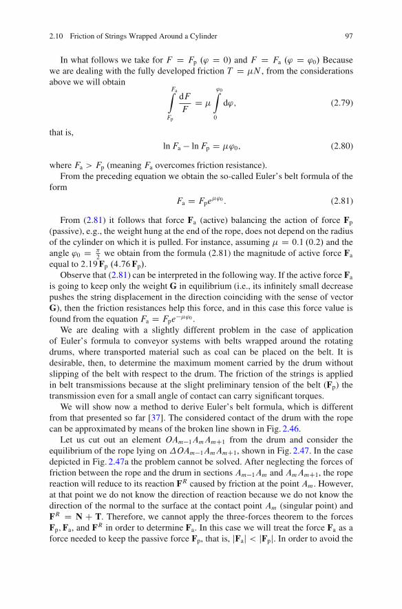
2.10 Friction of Strings Wrapped Around a Cylinder 97
In what follows we take for F D Fp .' D 0/ and F D Fa .' D '0/ Becausewe are dealing with the fully developed friction T D �N , from the considerationsabove we will obtain
FaZ
Fp
dF
FD �
'0Z
0
d'; (2.79)
that is,
lnFa � lnFp D �'0; (2.80)
where Fa > Fp (meaning Fa overcomes friction resistance).From the preceding equation we obtain the so-called Euler’s belt formula of the
form
Fa D Fpe�'0 : (2.81)
From (2.81) it follows that force Fa (active) balancing the action of force Fp
(passive), e.g., the weight hung at the end of the rope, does not depend on the radiusof the cylinder on which it is pulled. For instance, assuming � D 0:1 .0:2/ and theangle '0 D �
2we obtain from the formula (2.81) the magnitude of active force Fa
equal to 2:19Fp .4:76Fp/.Observe that (2.81) can be interpreted in the following way. If the active force Fa
is going to keep only the weight G in equilibrium (i.e., its infinitely small decreasepushes the string displacement in the direction coinciding with the sense of vectorG), then the friction resistances help this force, and in this case this force value isfound from the equation Fa D Fpe
��'0 .We are dealing with a slightly different problem in the case of application
of Euler’s formula to conveyor systems with belts wrapped around the rotatingdrums, where transported material such as coal can be placed on the belt. It isdesirable, then, to determine the maximum moment carried by the drum withoutslipping of the belt with respect to the drum. The friction of the strings is appliedin belt transmissions because at the slight preliminary tension of the belt (Fp) thetransmission even for a small angle of contact can carry significant torques.
We will show now a method to derive Euler’s belt formula, which is differentfrom that presented so far [37]. The considered contact of the drum with the ropecan be approximated by means of the broken line shown in Fig. 2.46.
Let us cut out an element OAm�1AmAmC1 from the drum and consider theequilibrium of the rope lying on �OAm�1AmAmC1, shown in Fig. 2.47. In the casedepicted in Fig. 2.47a the problem cannot be solved. After neglecting the forces offriction between the rope and the drum in sections Am�1Am and AmAmC1, the ropereaction will reduce to its reaction FR caused by friction at the point Am. However,at that point we do not know the direction of reaction because we do not know thedirection of the normal to the surface at the contact point Am (singular point) andFR D N C T. Therefore, we cannot apply the three-forces theorem to the forcesFp;Fa, and FR in order to determine Fa. In this case we will treat the force Fa as aforce needed to keep the passive force Fp, that is, jFaj < jFpj. In order to avoid the
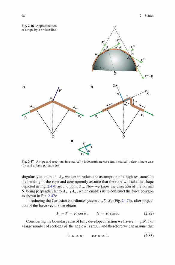
98 2 Statics
Fig. 2.46 Approximationof a rope by a broken line
Fig. 2.47 A rope and reactions in a statically indeterminate case (a), a statically determinate case(b), and a force polygon (c)
singularity at the point Am we can introduce the assumption of a high resistance tothe bending of the rope and consequently assume that the rope will take the shapedepicted in Fig. 2.47b around point Am. Now we know the direction of the normalN, being perpendicular to Am�1Am, which enables us to construct the force polygonas shown in Fig. 2.47c.
Introducing the Cartesian coordinate system AmX1X2 (Fig. 2.47b), after projec-tion of the force vectors we obtain
Fp � T D Fa cos˛; N D Fa sin ˛: (2.82)
Considering the boundary case of fully developed friction we have T D �N . Fora large number of sectionsM the angle ˛ is small, and therefore we can assume that
sin˛ Š ˛; cos˛ Š 1: (2.83)
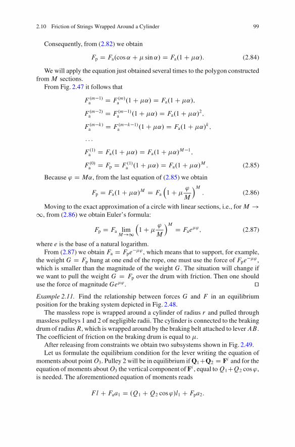
2.10 Friction of Strings Wrapped Around a Cylinder 99
Consequently, from (2.82) we obtain
Fp D Fa.cos˛ C � sin ˛/ D Fa.1C �˛/: (2.84)
We will apply the equation just obtained several times to the polygon constructedfromM sections.
From Fig. 2.47 it follows that
F .m�1/a D F .m/
a .1C �˛/ D Fa.1C �˛/;
F .m�2/a D F .m�1/
a .1C �˛/ D Fa.1C �˛/2;
F .m�k/a D F .m�k�1/
a .1C �˛/ D Fa.1C �˛/k;
: : :
F .1/a D Fa.1C �˛/ D Fa.1C �˛/M�1;
F .0/a D Fp D F .1/
a .1C �˛/ D Fa.1C �˛/M : (2.85)
Because ' D M˛, from the last equation of (2.85) we obtain
Fp D Fa.1C �˛/M D Fa
�1C �
'
M
�M: (2.86)
Moving to the exact approximation of a circle with linear sections, i.e., forM !1, from (2.86) we obtain Euler’s formula:
Fp D Fa limM!1
�1C �
'
M
�M D Fae�'; (2.87)
where e is the base of a natural logarithm.From (2.87) we obtain Fa D Fpe
��' , which means that to support, for example,the weight G D Fp hung at one end of the rope, one must use the force of Fpe
��' ,which is smaller than the magnitude of the weight G. The situation will change ifwe want to pull the weight G D Fp over the drum with friction. Then one shoulduse the force of magnitudeGe�' . utExample 2.11. Find the relationship between forces G and F in an equilibriumposition for the braking system depicted in Fig. 2.48.
The massless rope is wrapped around a cylinder of radius r and pulled throughmassless pulleys 1 and 2 of negligible radii. The cylinder is connected to the brakingdrum of radiusR, which is wrapped around by the braking belt attached to leverAB .The coefficient of friction on the braking drum is equal to �.
After releasing from constraints we obtain two subsystems shown in Fig. 2.49.Let us formulate the equilibrium condition for the lever writing the equation of
moments about pointO3. Pulley 2 will be in equilibrium if Q1CQ2 D Fi and for theequation of moments aboutO3 the vertical component of Fi , equal toQ1CQ2 cos',is needed. The aforementioned equation of moments reads
F l C Faa1 D .Q1 CQ2 cos'/l1 C Fpa2:
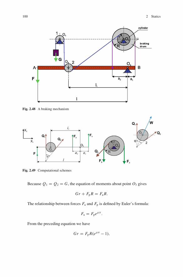
100 2 Statics
Fig. 2.48 A braking mechanism
Fig. 2.49 Computational schemes
Because Q1 D Q2 D G, the equation of moments about point O3 gives
Gr C FpR D FaR:
The relationship between forces Fa and Fp is defined by Euler’s formula:
Fa D Fpe��:
From the preceding equation we have
Gr D FpR.e�� � 1/;
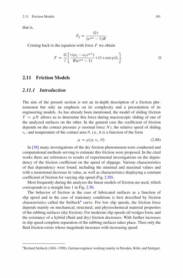
2.11 Friction Models 101
that is,
Fp D Gr
.e�� � 1/R:
Coming back to the equation with force F we obtain
F D G
l
�r.a2 � a1e��/R.e�� � 1/ C.1Ccos'/l1
: ut
2.11 Friction Models
2.11.1 Introduction
The aim of the present section is not an in-depth description of a friction phe-nomenon but only an emphasis on its complexity and a presentation of itsengineering models. As has already been mentioned, the model of sliding frictionT D �N allows us to determine this force during macroscopic sliding of one ofthe analyzed surfaces on the other. In the general case the coefficient of frictiondepends on the contact pressure p (normal force N ), the relative speed of slidingvr , and temperature of the contact area � , i.e., it is a function of the form
� D �.p; vr ; �/: (2.88)
In [38] many investigations of the dry friction phenomenon were conducted andcomputational methods serving to estimate this friction were proposed. In the citedworks there are references to results of experimental investigations on the depen-dency of the friction coefficient on the speed of slippage. Various characteristicsof that dependency were found, including the minimal and maximal values andwith a monotonal decrease in value, as well as characteristics displaying a constantcoefficient of friction for varying slip speed (Fig. 2.50).
Most frequently during the analyses the linear models of friction are used, whichcorresponds to a straight line 1 in Fig. 2.50.
The behavior of friction in the case of lubricated surfaces as a function ofslip speed and in the case of stationary conditions is best described by frictioncharacteristics called the Stribeck6 curve. For low slip speeds, the friction forcedepends mainly on mechanical, structural, and physiochemical material propertiesof the rubbing surfaces (dry friction). For moderate slip speeds oil wedges form, andthe resistance of a hybrid (fluid and dry) friction decreases. With further increasesin slip speed complete separation of the rubbing surfaces takes place. Then only thefluid friction exists whose magnitude increases with increasing speed.
6Richard Stribeck (1861–1950), German engineer working mainly in Dresden, Koln, and Stuttgart.
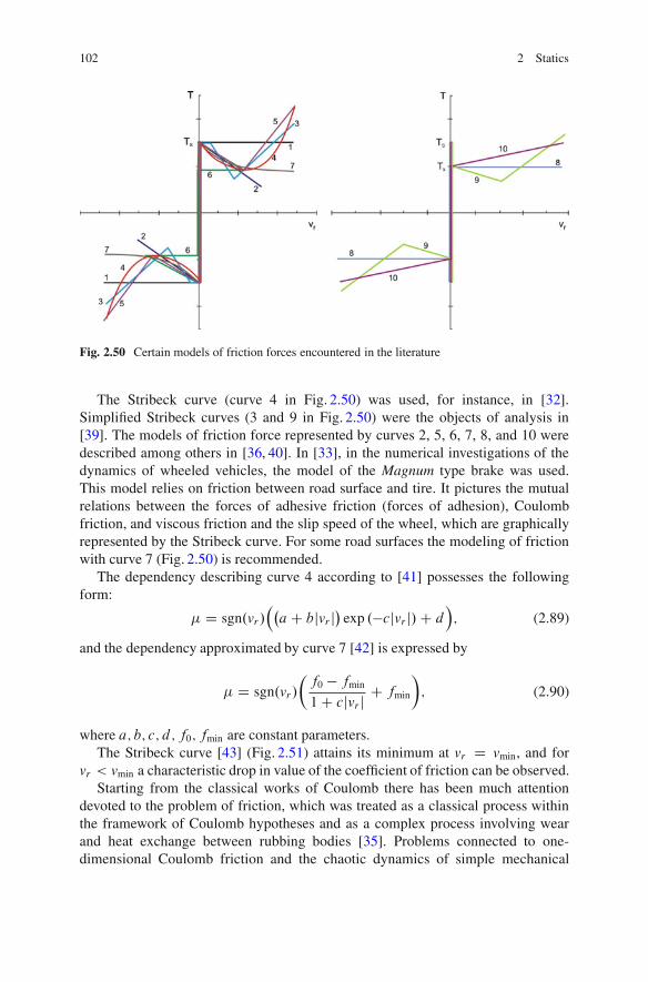
102 2 Statics
Fig. 2.50 Certain models of friction forces encountered in the literature
The Stribeck curve (curve 4 in Fig. 2.50) was used, for instance, in [32].Simplified Stribeck curves (3 and 9 in Fig. 2.50) were the objects of analysis in[39]. The models of friction force represented by curves 2, 5, 6, 7, 8, and 10 weredescribed among others in [36, 40]. In [33], in the numerical investigations of thedynamics of wheeled vehicles, the model of the Magnum type brake was used.This model relies on friction between road surface and tire. It pictures the mutualrelations between the forces of adhesive friction (forces of adhesion), Coulombfriction, and viscous friction and the slip speed of the wheel, which are graphicallyrepresented by the Stribeck curve. For some road surfaces the modeling of frictionwith curve 7 (Fig. 2.50) is recommended.
The dependency describing curve 4 according to [41] possesses the followingform:
� D sgn.vr /��aC bjvr j
�exp .�cjvr j/C d
�; (2.89)
and the dependency approximated by curve 7 [42] is expressed by
� D sgn.vr /
f0 � fmin
1C cjvr j C fmin
�; (2.90)
where a; b; c; d; f0; fmin are constant parameters.The Stribeck curve [43] (Fig. 2.51) attains its minimum at vr D vmin, and for
vr < vmin a characteristic drop in value of the coefficient of friction can be observed.Starting from the classical works of Coulomb there has been much attention
devoted to the problem of friction, which was treated as a classical process withinthe framework of Coulomb hypotheses and as a complex process involving wearand heat exchange between rubbing bodies [35]. Problems connected to one-dimensional Coulomb friction and the chaotic dynamics of simple mechanical
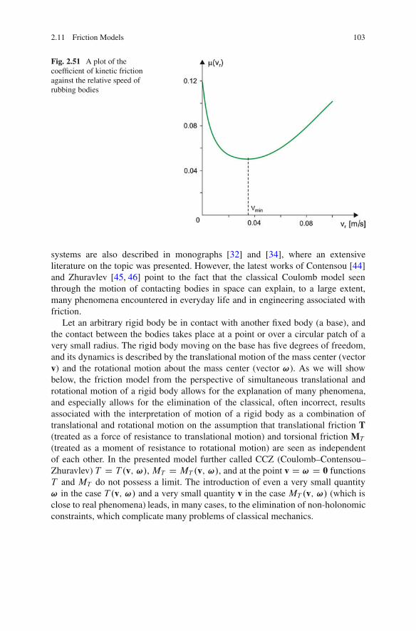
2.11 Friction Models 103
Fig. 2.51 A plot of thecoefficient of kinetic frictionagainst the relative speed ofrubbing bodies
systems are also described in monographs [32] and [34], where an extensiveliterature on the topic was presented. However, the latest works of Contensou [44]and Zhuravlev [45, 46] point to the fact that the classical Coulomb model seenthrough the motion of contacting bodies in space can explain, to a large extent,many phenomena encountered in everyday life and in engineering associated withfriction.
Let an arbitrary rigid body be in contact with another fixed body (a base), andthe contact between the bodies takes place at a point or over a circular patch of avery small radius. The rigid body moving on the base has five degrees of freedom,and its dynamics is described by the translational motion of the mass center (vectorv) and the rotational motion about the mass center (vector !). As we will showbelow, the friction model from the perspective of simultaneous translational androtational motion of a rigid body allows for the explanation of many phenomena,and especially allows for the elimination of the classical, often incorrect, resultsassociated with the interpretation of motion of a rigid body as a combination oftranslational and rotational motion on the assumption that translational friction T(treated as a force of resistance to translational motion) and torsional friction MT
(treated as a moment of resistance to rotational motion) are seen as independentof each other. In the presented model further called CCZ (Coulomb–Contensou–Zhuravlev) T D T .v; !/, MT D MT .v; !/, and at the point v D ! D 0 functionsT and MT do not possess a limit. The introduction of even a very small quantity! in the case T .v; !/ and a very small quantity v in the case MT .v; !/ (which isclose to real phenomena) leads, in many cases, to the elimination of non-holonomicconstraints, which complicate many problems of classical mechanics.
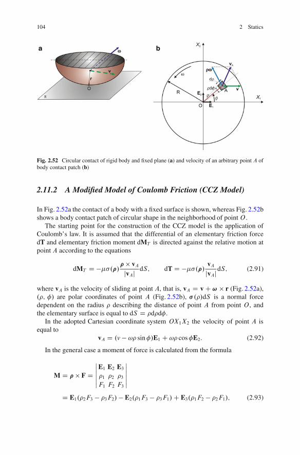
104 2 Statics
Fig. 2.52 Circular contact of rigid body and fixed plane (a) and velocity of an arbitrary point A ofbody contact patch (b)
2.11.2 A Modified Model of Coulomb Friction (CCZ Model)
In Fig. 2.52a the contact of a body with a fixed surface is shown, whereas Fig. 2.52bshows a body contact patch of circular shape in the neighborhood of pointO .
The starting point for the construction of the CCZ model is the application ofCoulomb’s law. It is assumed that the differential of an elementary friction forcedT and elementary friction moment dMT is directed against the relative motion atpoint A according to the equations
dMT D ���.�/� � vAjvAj dS; dT D ���.�/ vA
jvAjdS; (2.91)
where vA is the velocity of sliding at point A, that is, vA D v C ! � r (Fig. 2.52a),.; / are polar coordinates of point A (Fig. 2.52b), � ./dS is a normal forcedependent on the radius describing the distance of point A from point O , andthe elementary surface is equal to dS D dd.
In the adopted Cartesian coordinate system OX1X2 the velocity of point A isequal to
vA D .v � ! sin/E1 C ! cosE2: (2.92)
In the general case a moment of force is calculated from the formula
M D � � F DˇˇˇE1 E2 E31 2 3F1 F2 F3
ˇˇˇ
D E1.2F3 � 3F2/ � E2.1F3 � 3F1/C E3.1F2 � 2F1/; (2.93)
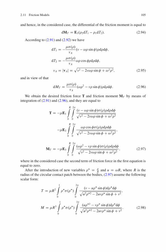
2.11 Friction Models 105
and hence, in the considered case, the differential of the friction moment is equal to
dMT D E3.2dT1 � 1dT2/: (2.94)
According to (2.91) and (2.92) we have
dT1 D ���./vA
.v � ! sin /dd;
dT2 D ���./vA
! cosdd;
vA D jvAj Dp
v2 � 2v! sin C !22; (2.95)
and in view of that
dMT D ��./
vA.!2 � v sin/dd: (2.96)
We obtain the desired friction force T and friction moment MT by means ofintegration of (2.91) and (2.96), and they are equal to
T D ��E1
RZ
0
2�Z
0
.v � ! sin /�./ddpv2 � 2v! sin C !22
��E2
RZ
0
2�Z
0
! cos�./ddp
v2 � 2v! sin C !22;
MT D ��E3
RZ
0
2�Z
0
.!2 � v sin /�./ddp
v2 � 2v! sin C !22; (2.97)
where in the considered case the second term of friction force in the first equation isequal to zero.
After the introduction of new variables � D
Rand u D !R, where R is the
radius of the circular contact patch between the bodies, (2.97) assume the followingscalar form:
T D �R21Z
0
��.�/2�Z
0
.v � u� sin /d�dp
u2�2 � 2uv� sin C v2;
M D �R31Z
0
��.�/2�Z
0
.u�2 � v� sin /d�dpu2�2 � 2uv� sin C v2
: (2.98)
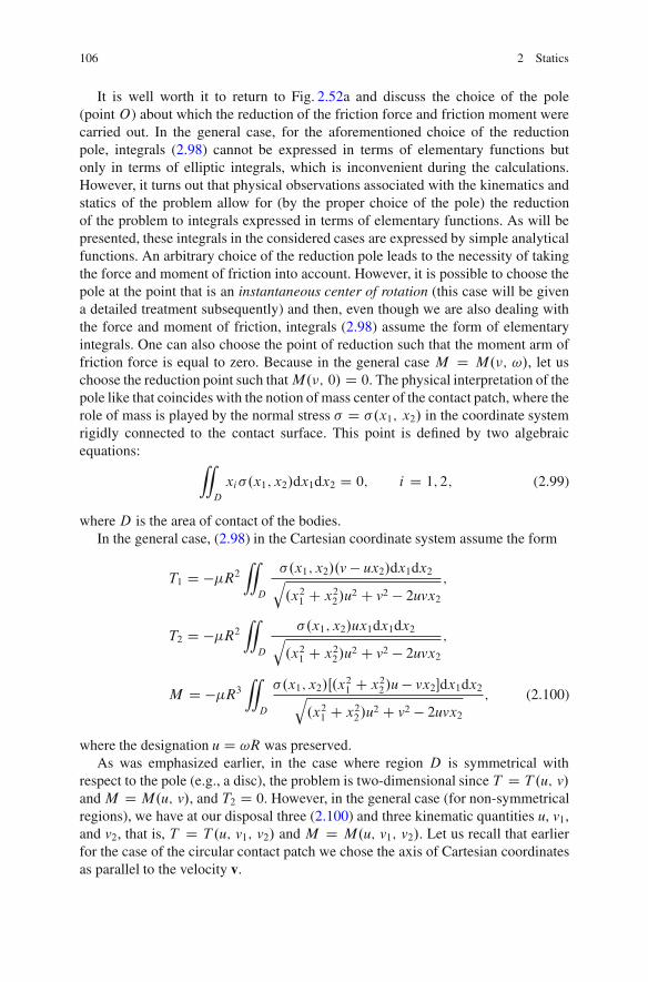
106 2 Statics
It is well worth it to return to Fig. 2.52a and discuss the choice of the pole(point O) about which the reduction of the friction force and friction moment werecarried out. In the general case, for the aforementioned choice of the reductionpole, integrals (2.98) cannot be expressed in terms of elementary functions butonly in terms of elliptic integrals, which is inconvenient during the calculations.However, it turns out that physical observations associated with the kinematics andstatics of the problem allow for (by the proper choice of the pole) the reductionof the problem to integrals expressed in terms of elementary functions. As will bepresented, these integrals in the considered cases are expressed by simple analyticalfunctions. An arbitrary choice of the reduction pole leads to the necessity of takingthe force and moment of friction into account. However, it is possible to choose thepole at the point that is an instantaneous center of rotation (this case will be givena detailed treatment subsequently) and then, even though we are also dealing withthe force and moment of friction, integrals (2.98) assume the form of elementaryintegrals. One can also choose the point of reduction such that the moment arm offriction force is equal to zero. Because in the general case M D M.�; !/, let uschoose the reduction point such thatM.�; 0/ D 0. The physical interpretation of thepole like that coincides with the notion of mass center of the contact patch, where therole of mass is played by the normal stress � D �.x1; x2/ in the coordinate systemrigidly connected to the contact surface. This point is defined by two algebraicequations:
“
D
xi�.x1; x2/dx1dx2 D 0; i D 1; 2; (2.99)
whereD is the area of contact of the bodies.In the general case, (2.98) in the Cartesian coordinate system assume the form
T1 D ��R2“
D
�.x1; x2/.v � ux2/dx1dx2q.x21 C x22/u
2 C v2 � 2uvx2;
T2 D ��R2“
D
�.x1; x2/ux1dx1dx2q.x21 C x22/u
2 C v2 � 2uvx2;
M D ��R3“
D
�.x1; x2/Œ.x21 C x22/u � vx2�dx1dx2q
.x21 C x22/u2 C v2 � 2uvx2
; (2.100)
where the designation u D !R was preserved.As was emphasized earlier, in the case where region D is symmetrical with
respect to the pole (e.g., a disc), the problem is two-dimensional since T D T .u; v/andM D M.u; v/, and T2 D 0. However, in the general case (for non-symmetricalregions), we have at our disposal three (2.100) and three kinematic quantities u, v1,and v2, that is, T D T .u; v1; v2/ and M D M.u; v1; v2/. Let us recall that earlierfor the case of the circular contact patch we chose the axis of Cartesian coordinatesas parallel to the velocity v.
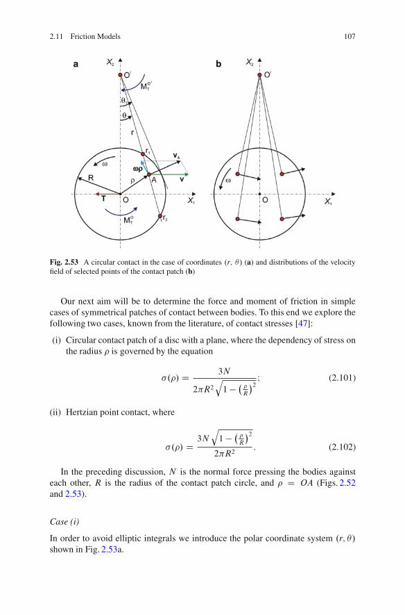
2.11 Friction Models 107
Fig. 2.53 A circular contact in the case of coordinates .r; �/ (a) and distributions of the velocityfield of selected points of the contact patch (b)
Our next aim will be to determine the force and moment of friction in simplecases of symmetrical patches of contact between bodies. To this end we explore thefollowing two cases, known from the literature, of contact stresses [47]:
(i) Circular contact patch of a disc with a plane, where the dependency of stress onthe radius is governed by the equation
�./ D 3N
2�R2q1 � �
R
�2 I (2.101)
(ii) Hertzian point contact, where
�./ D3N
q1 � �
R
�2
2�R2: (2.102)
In the preceding discussion, N is the normal force pressing the bodies againsteach other, R is the radius of the contact patch circle, and D OA (Figs. 2.52and 2.53).
Case (i)
In order to avoid elliptic integrals we introduce the polar coordinate system .r; �/
shown in Fig. 2.53a.
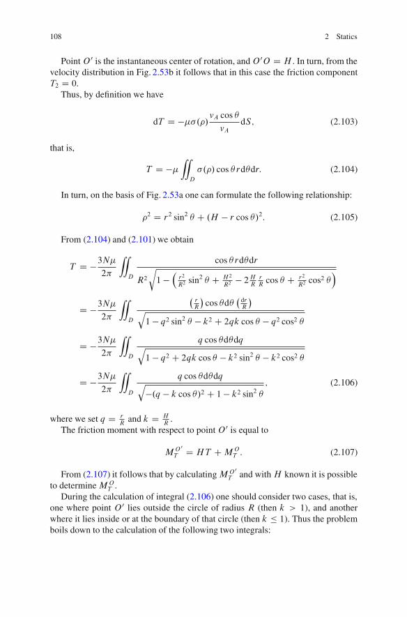
108 2 Statics
PointO 0 is the instantaneous center of rotation, andO 0O D H . In turn, from thevelocity distribution in Fig. 2.53b it follows that in this case the friction componentT2 D 0.
Thus, by definition we have
dT D ���./vA cos �
vAdS; (2.103)
that is,
T D ��“
D
�./ cos � rd�dr: (2.104)
In turn, on the basis of Fig. 2.53a one can formulate the following relationship:
2 D r2 sin2 � C .H � r cos �/2: (2.105)
From (2.104) and (2.101) we obtain
T D �3N�2�
“
D
cos � rd�dr
R2
r1 �
�r2
R2sin2 � C H2
R2� 2H
RrR
cos � C r2
R2cos2 �
�
D �3N�2�
“
D
�rR
�cos �d�
�drR
�q1 � q2 sin2 � � k2 C 2qk cos � � q2 cos2 �
D �3N�2�
“
D
q cos �d�dqq1 � q2 C 2qk cos � � k2 sin2 � � k2 cos2 �
D �3N�2�
“
D
q cos �d�dqq
�.q � k cos �/2 C 1 � k2 sin2 �; (2.106)
where we set q D rR
and k D HR
.The friction moment with respect to pointO 0 is equal to
MO 0
T D HT CMOT : (2.107)
From (2.107) it follows that by calculatingMO 0
T and withH known it is possibleto determineMO
T .During the calculation of integral (2.106) one should consider two cases, that is,
one where point O 0 lies outside the circle of radius R (then k > 1), and anotherwhere it lies inside or at the boundary of that circle (then k � 1). Thus the problemboils down to the calculation of the following two integrals:
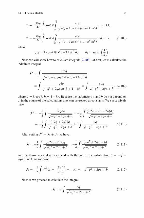
2.11 Friction Models 109
T D �3N�4�
�Z
0
cos �d�
q2Z
q1
qdqq�.q � k cos �/2 C 1� k2 sin2 �
; .k � 1/;
T D �3N�2�
�1Z
0
cos �d�
q2Z
q1
qdqq�.q � k cos �/2 C 1� k2 sin2 �
; .k > 1/; (2.108)
where
q1;2 D k cos � �p1 � k2 sin2 � ; �1 D arcsin
1
k
�:
Now, we will show how to calculate integrals (2.108). At first, let us calculate theindefinite integral
J � DZ
qdqq�.q � k cos �/2 C 1 � k2 sin2 �
DZ
qdqp�q2 C 2qk cos � C 1 � k2 DZ
qdqp�q2 C 2qaC b; (2.109)
where a D k cos � , b D 1 � k2. Because the parameters a and b do not depend onq, in the course of the calculations they can be treated as constants. We successivelyhave
J � D �12
Z �2qdqp�q2 C 2qaC bD �1
2
Z.�2q C 2a � 2a/dqp�q2 C 2qaC b
D �12
Z.�2q C 2a/dqp�q2 C 2qaC b
C a
Zdq
p�q2 C 2qa C b: (2.110)
After setting J � D J1 C J2 we have
J1 D �12
Z.�2q C 2a/dqp�q2 C 2qaC b
D �12
Zd.�q2 C 2qa C b/p�q2 C 2qaC b
; (2.111)
and the above integral is calculated with the aid of the substitution t D �q2C2qaC b. Thus we have
J1 D �12
Zt� 1
2 dt D �12
t� 12
12
D �pt D �
p�q2 C 2qa C b: (2.112)
Now as we proceed to calculate the integral
J2 D a
Zdqp�q2 C 2qaC b
: (2.113)
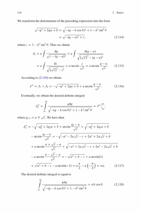
110 2 Statics
We transform the denominator of the preceding expression into the form
p�q2 C 2qa C b D
q�.q � k cos �/2 C 1 � k2 sin2 �
Dp
�.q � a/2 C c; (2.114)
where c D 1� k2 sin2 � . Thus we obtain
J2 D a
Zdq
pc � .q � a/2 D a
Zd.q � a/
q�pc�2 � .q � a/2
D a
Zdz
q�pc�2 � z2
D a arcsinzpc
D a arcsinq � apc: (2.115)
According to (2.110) we obtain
J � D J1 C J2 D �p
�q2 C 2qaC b C a arcsinq � apc: (2.116)
Eventually, we obtain the desired definite integral
J �0 D
q2Z
q1
qdqq�.q � k cos �/2 C 1 � k2 sin2 �
D J �ˇˇq2
q1;
where q1;2 D a � pc. We have then
J �0 D �
q�q22 C 2q2a C b C arcsin
q2 � apc
Cq
�q21 C 2q1aC b
� arcsinq1 � ap
cD �
q�a2 � 2ap
c � c C 2a2 C 2apc C b
C a arcsina C p
c � apc
Cq
�a2 C 2apc � c C 2a2 � 2ap
c C b
� a arcsina � p
c � apc
D �pa2 C b � c C a arcsin.1/
Cpa2 C b � c � a arcsin.�1/ D a
�
2� a
���2
�D �a: (2.117)
The desired definite integral is equal to
q2Z
q1
qdqq
�.q � k cos �/2 C 1 � k2 sin2 �D �k cos �: (2.118)
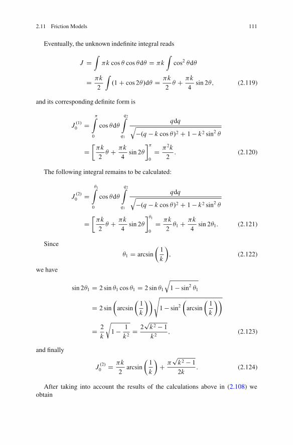
2.11 Friction Models 111
Eventually, the unknown indefinite integral reads
J DZ�k cos � cos �d� D �k
Zcos2 �d�
D �k
2
Z.1C cos 2�/d� D �k
2� C �k
4sin 2�; (2.119)
and its corresponding definite form is
J.1/0 D
�Z
0
cos �d�
q2Z
q1
qdqq�.q � k cos �/2 C 1 � k2 sin2 �
D��k
2� C �k
4sin 2�
�
0
D �2k
2: (2.120)
The following integral remains to be calculated:
J.2/0 D
�1Z
0
cos �d�
q2Z
q1
qdqq�.q � k cos �/2 C 1 � k2 sin2 �
D��k
2� C �k
4sin 2�
�1
0
D �k
2�1 C �k
4sin 2�1: (2.121)
Since
�1 D arcsin
1
k
�; (2.122)
we have
sin 2�1 D 2 sin �1 cos �1 D 2 sin �1
q1 � sin2 �1
D 2 sin
arcsin
1
k
��s
1 � sin2
arcsin
1
k
��
D 2
k
r1 � 1
k2D 2
pk2 � 1
k2; (2.123)
and finally
J.2/0 D �k
2arcsin
1
k
�C �
pk2 � 1
2k: (2.124)
After taking into account the results of the calculations above in (2.108) weobtain
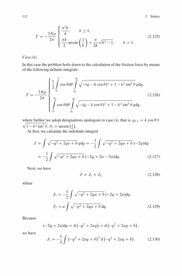
112 2 Statics
T D �3N�2�
8ˆ<
ˆ:
�2k
4; k � 1;
�k
2arcsin
1
k
�C �
2k
pk2 � 1; k > 1:
(2.125)
Case (ii)
In this case the problem boils down to the calculation of the friction force by meansof the following definite integrals:
T D �3N�2�
8ˆˆˆ<
ˆˆˆ:
1
2
�Z
0
cos �d�
q2Z
q1
q�.q � k cos �/2 C 1 � k2 sin2 � qdq;
�1Z
0
cos �d�
q2Z
q1
q�.q � k cos �/2 C 1� k2 sin2 � qdq;
(2.126)
where further we adopt designations analogous to case (i), that is, q1;2 D k cos ��p1 � k2 sin2 � , �1 D arcsin
�1k
�.
At first, we calculate the indefinite integral
J DZ p
�q2 C 2qa C b qdq D �12
Z p�q2 C 2qaC b .�2q/dq
D �12
Z p�q2 C 2qaC b .�2q C 2a � 2a/dq: (2.127)
Next, we have
J D J1 C J2; (2.128)
where
J1 D �12
Z p�q2 C 2qa C b .�2q C 2a/dq;
J2 D a
Z p�q2 C 2qaC b dq: (2.129)
Because
.�2q C 2a/dq D d��q2 C 2aq
� D d��q2 C 2aq C b
�;
we have
J1 D �12
Z ��q2 C 2aq C b� 12 d��q2 C 2aq C b
�: (2.130)
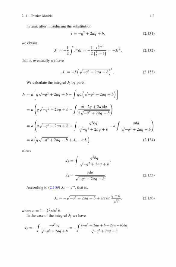
2.11 Friction Models 113
In turn, after introducing the substitution
t D �q2 C 2aq C b; (2.131)
we obtain
J1 D �12
Zt12 dt D �1
2
t12C1
�12
C 1� D �3t 32 ; (2.132)
that is, eventually we have
J1 D �3�p
�q2 C 2aq C b�3: (2.133)
We calculate the integral J2 by parts:
J2 D a
�qp
�q2 C 2aq C b �Zqd�p
�q2 C 2aq C b�
D a
qp
�q2 C 2aq C b �Z
q.�2q C 2a/dq
2p�q2 C 2aq C b
!
D a
qp
�q2 C 2aq C b CZ
q2dqp�q2 C 2aq C b� a
Zqdqp�q2 C 2aq C b
!
D a�qp
�q2 C 2aq C b C J3 � aJ4
�; (2.134)
where
J3 DZ
q2dqp�q2 C 2aq C b;
J4 D qdqp�q2 C 2aq C b
: (2.135)
According to (2.109) J4 D J �, that is,
J4 D �p
�q2 C 2aq C b C arcsinq � apc; (2.136)
where c D 1� k2 sin2 � .In the case of the integral J3 we have
J3 D �Z �q2dqp�q2 C 2aq C b
D �Z.�q2 C 2qaC b � 2qa � b/dq
p�q2 C 2aq C b
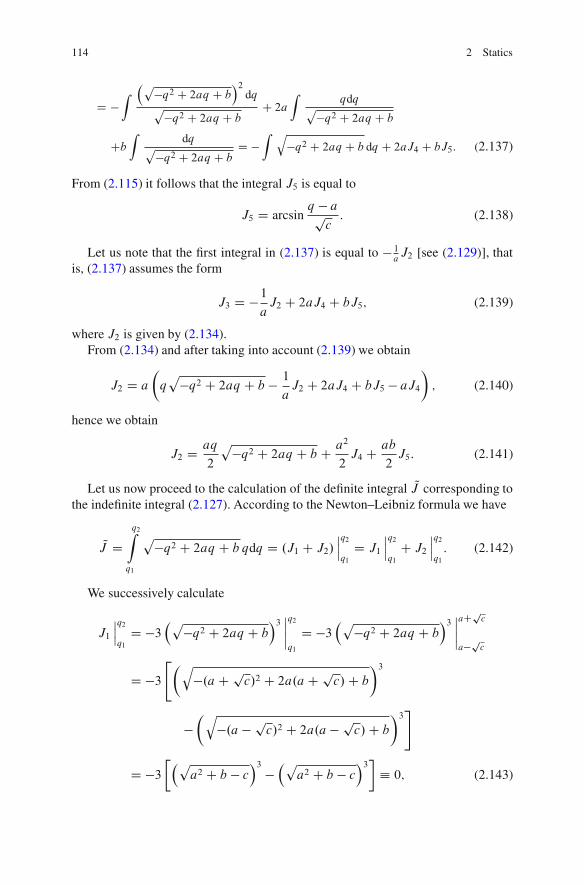
114 2 Statics
D �Z�p
�q2 C 2aq C b�2
dqp
�q2 C 2aq C bC 2a
Zqdqp
�q2 C 2aq C b
CbZ
dqp�q2 C 2aq C b
D �Z q
�q2 C 2aq C b dq C 2aJ4 C bJ5: (2.137)
From (2.115) it follows that the integral J5 is equal to
J5 D arcsinq � apc: (2.138)
Let us note that the first integral in (2.137) is equal to � 1aJ2 [see (2.129)], that
is, (2.137) assumes the form
J3 D �1aJ2 C 2aJ4 C bJ5; (2.139)
where J2 is given by (2.134).From (2.134) and after taking into account (2.139) we obtain
J2 D a
qp
�q2 C 2aq C b � 1
aJ2 C 2aJ4 C bJ5 � aJ4
�; (2.140)
hence we obtain
J2 D aq
2
p�q2 C 2aq C b C a2
2J4 C ab
2J5: (2.141)
Let us now proceed to the calculation of the definite integral QJ corresponding tothe indefinite integral (2.127). According to the Newton–Leibniz formula we have
QJ Dq2Z
q1
p�q2 C 2aq C b qdq D .J1 C J2/
ˇˇq2
q1D J1
ˇˇq2
q1C J2
ˇˇq2
q1: (2.142)
We successively calculate
J1
ˇˇq2
q1D �3
�p�q2 C 2aq C b
�3 ˇˇq2
q1
D �3�p
�q2 C 2aq C b�3 ˇˇ
aCpc
a�pc
D �3"q
�.a C pc/2 C 2a.aC p
c/C b
�3
�q
�.a � pc/2 C 2a.a � p
c/C b
�3#
D �3��p
a2 C b � c�3 �
�pa2 C b � c
�3 � 0; (2.143)
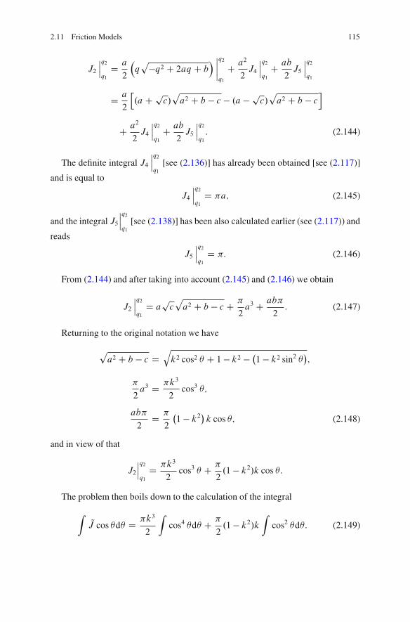
2.11 Friction Models 115
J2
ˇˇq2
q1D a
2
�qp
�q2 C 2aq C b� ˇˇq2
q1
C a2
2J4
ˇˇq2
q1C ab
2J5
ˇˇq2
q1
D a
2
h.a C p
c/pa2 C b � c � .a � p
c/pa2 C b � c
i
C a2
2J4
ˇˇq2
q1C ab
2J5
ˇˇq2
q1: (2.144)
The definite integral J4ˇˇq2
q1[see (2.136)] has already been obtained [see (2.117)]
and is equal to
J4
ˇˇq2
q1D �a; (2.145)
and the integral J5ˇˇq2
q1[see (2.138)] has been also calculated earlier (see (2.117)) and
reads
J5
ˇˇq2
q1D �: (2.146)
From (2.144) and after taking into account (2.145) and (2.146) we obtain
J2
ˇˇq2
q1D a
pcpa2 C b � c C �
2a3 C ab�
2: (2.147)
Returning to the original notation we have
pa2 C b � c D
qk2 cos2 � C 1 � k2 � �
1 � k2 sin2 ��;
�
2a3 D �k3
2cos3 �;
ab�
2D �
2
�1 � k2
�k cos �; (2.148)
and in view of that
J2
ˇˇq2
q1D �k3
2cos3 � C �
2.1 � k2/k cos �:
The problem then boils down to the calculation of the integral
ZQJ cos �d� D �k3
2
Zcos4 �d� C �
2.1� k2/k
Zcos2 �d�: (2.149)
116 2 Statics
The elementary integrals are calculated in the following way:
Zcos2 �d� D 1
2
Z.1C cos 2�/d� D �
2C 1
4sin 2�;
Zcos4 �d� D 1
4
Z.1C cos 2�/2d�
D 1
4
Z.1C 2 cos 2� C cos2 2�/d�
D 1
4� C 1
4sin 2� C 1
8
Z.1C cos 4�/d�
D 1
4� C 1
4sin 2� C �
8C 1
32sin 4�: (2.150)
In order to shorten the notation we calculate the following definite integrals:
�Z
0
cos2 �d� D�
2C 1
4sin 2�
� ˇˇ�
0
D �
2;
�1Z
0
cos2 �d� D�
2C 1
2sin �
p1 � sin2 �
� ˇˇarcsin 1
k
0
D 1
2arcsin
1
kC
pk2 � 1
2k2;
�Z
0
cos4 �d� D3�
8C 1
4sin 2� C 1
32sin 4�
� ˇˇ�
0
D 3�
8;
�1Z
0
cos4 �d� D3�
8C 1
2sin �
p1 � sin2 �
C1
8sin �
p1 � sin2 �.1 � 2 sin2 �/
� ˇˇarcsin 1
k
0
D 3
8arcsin
1
kC
pk2 � 12k2
C .k2 � 1/pk2 � 1
8k4
D 3
8arcsin
1
kC .5k2 � 2/pk2 � 1
8k4: (2.151)
From (2.126) we eventually obtain
2.11 Friction Models 117
T D �3N�2�
8ˆˆˆˆˆˆ<
ˆˆˆˆˆˆ:
�Z
0
cos �d�
q2Z
q1
q�.q � k cos �/2 C 1 � k2 sin2 � qdq
D �2k
16
�4 � k2
� I .k � 1/
�1Z
0
cos �d�
q2Z
q1
q�.q � k cos �/2 C 1 � k2 sin2 � qdq
D �k
16
�4 � k2� arcsin
1
kC �
�2C k2
�pk2 � 1
16kI .k > 1/:
(2.152)
Let us now return to the friction model presented in Figs. 2.52 and 2.53. Thefriction moment about point O 0 (the instantaneous center of rotation) we obtain byexploiting (2.106), where additionally the numerator of the integrand is multipliedby Rr
RD Rq to obtain
MO 0
T D �NR
8ˆˆˆ<
ˆˆˆ:
1
2
�Z
0
d�
q2Z
q1
q2dqq�.q � k cos �/2 C 1 � k2 sin2 �
; .k � 1/;
�1Z
0
d�
q2Z
q1
q2dqq�.q � k cos �/2 C 1 � k2 sin2 �
; .k > 1/:
(2.153)After using the previous calculations [see (2.135)] we obtain
MO 0
T D �NR
8ˆ<
ˆ:
�2.2C k2/
8; k � 1;
�2.2C k2/
4arcsin
1
kC 3�
4
pk2 � 1; k > 1:
(2.154)
Our aim is to determine the moment of friction forces with respect to point O ,which, according to the designations presented in Fig. 2.53a, is equal to
MO 0
T �MOT �HT D 0; (2.155)
that is,MOT D MO 0
T �HT; (2.156)
where the friction force T is given by (2.106).
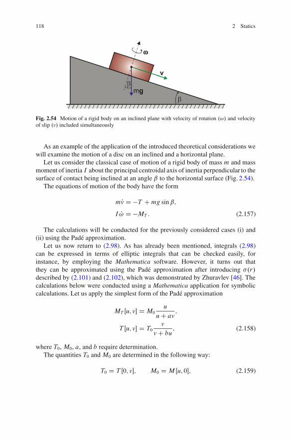
118 2 Statics
Fig. 2.54 Motion of a rigid body on an inclined plane with velocity of rotation .!/ and velocityof slip .v/ included simultaneously
As an example of the application of the introduced theoretical considerations wewill examine the motion of a disc on an inclined and a horizontal plane.
Let us consider the classical case of motion of a rigid body of mass m and massmoment of inertia I about the principal centroidal axis of inertia perpendicular to thesurface of contact being inclined at an angle ˇ to the horizontal surface (Fig. 2.54).
The equations of motion of the body have the form
mPv D �T Cmg sinˇ;
I P! D �MT : (2.157)
The calculations will be conducted for the previously considered cases (i) and(ii) using the Pade approximation.
Let us now return to (2.98). As has already been mentioned, integrals (2.98)can be expressed in terms of elliptic integrals that can be checked easily, forinstance, by employing the Mathematica software. However, it turns out thatthey can be approximated using the Pade approximation after introducing �.r/described by (2.101) and (2.102), which was demonstrated by Zhuravlev [46]. Thecalculations below were conducted using a Mathematica application for symboliccalculations. Let us apply the simplest form of the Pade approximation
MT Œu; v� D M0
u
u C av;
T Œu; v� D T0v
v C bu; (2.158)
where T0, M0, a, and b require determination.The quantities T0 andM0 are determined in the following way:
T0 D T Œ0; v�; M0 D MŒu; 0�; (2.159)
2.11 Friction Models 119
and from (2.98) we find
T0 D �R21Z
0
��.�/2�Z
0
d�d D 2��R21Z
0
��.�/d�;
M0 D �R3
1Z
0
��.�/2�Z
0
�d�d D 2��R3
1Z
0
�2�.�/d�: (2.160)
The quantities a and b are obtained after the differentiation of (2.158) and (2.98)with respect to variables u and v. After adequate differentiation of the equations wehave
@T
@vŒu; 0� D T0
bu;
@M
@uŒ0; v� D M0
av; (2.161)
and after differentiation of (2.98) we obtain
@T
@vŒu; 0� D R�
u
1Z
0
�.�/d�;
@M
@uŒ0; v� D �
Rv
1Z
0
�3�.�/d�: (2.162)
After equating (2.161) and (2.162) by sides we obtain the unknown coefficients
a D21R0
�2�.�/d�
1R
0
�3�.�/d�; b D
21R0
��.�/d�
1R
0
�.�/d�: (2.163)
The desired coefficients were found using Mathematica.Equations (2.157), after taking into account the Pade approximation, assume the
form
mdv
dtD � T0v
jvj C buCmg sinˇ;
Idu
dtD � RM0u
juj C av; (2.164)
where u D R!.In the case of a contact over the circular patch (case i) R denotes the radius, and
in the case of the point contact R ! 0.
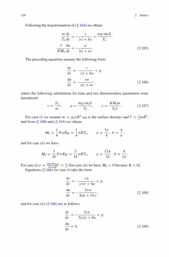
120 2 Statics
Following the transformation of (2.164) we obtain
m
T0
dv
dtD � v
jvj C buC mg sinˇ
T0;
I
RM0
du
dtD � u
juj C av: (2.165)
The preceding equations assume the following form:
dv
d�D � v
jvj C buC p;
du
d�D � eu
juj C av; (2.166)
where the following substitution for time and two dimensionless parameters wereintroduced:
� D T0
mt; p D mg sinˇ
T0; e D RM0m
T0I: (2.167)
For case (i) we assume m D 0�R2 (0 is the surface density) and I D 1
2mR2,
and from (2.160) and (2.163) we obtain
M0 D 1
4N�R� D 1
4�RT0; a D 3�
4; b D 4
�;
and for case (ii) we have
M0 D 3
16N�R� D 3
16�RT0; a D 15�
16; b D 8
3�:
For case (i) e D 2R�RT0m4T0mR2
D �2
[for case (ii) we have M0 D 0 because R D 0].Equations (2.166) for case (i) take the form
dv
d�D � v�
jvj� C 4uC p;
du
d�D � 2�u
4juj C 3�v; (2.168)
and for case (ii) (2.166) are as follows:
dv
d�D � 3v�
3jvj� C 8uC p;
du
d�D 0: (2.169)
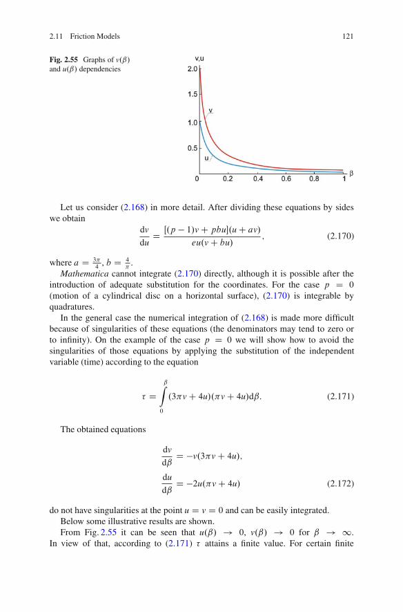
2.11 Friction Models 121
Fig. 2.55 Graphs of v.ˇ/and u.ˇ/ dependencies
Let us consider (2.168) in more detail. After dividing these equations by sideswe obtain
dv
duD Œ.p � 1/v C pbu�.u C av/
eu.v C bu/; (2.170)
where a D 3�4
, b D 4�
.Mathematica cannot integrate (2.170) directly, although it is possible after the
introduction of adequate substitution for the coordinates. For the case p D 0
(motion of a cylindrical disc on a horizontal surface), (2.170) is integrable byquadratures.
In the general case the numerical integration of (2.168) is made more difficultbecause of singularities of these equations (the denominators may tend to zero orto infinity). On the example of the case p D 0 we will show how to avoid thesingularities of those equations by applying the substitution of the independentvariable (time) according to the equation
� DˇZ
0
.3�v C 4u/.�v C 4u/dˇ: (2.171)
The obtained equations
dv
dˇD �v.3�v C 4u/;
du
dˇD �2u.�v C 4u/ (2.172)
do not have singularities at the point u D v D 0 and can be easily integrated.Below some illustrative results are shown.From Fig. 2.55 it can be seen that u.ˇ/ ! 0, v.ˇ/ ! 0 for ˇ ! 1.
In view of that, according to (2.171) � attains a finite value. For certain finite
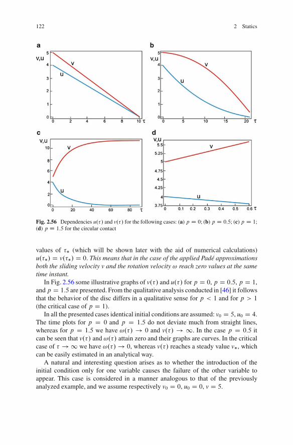
122 2 Statics
Fig. 2.56 Dependencies u.�/ and v.�/ for the following cases: (a) p D 0; (b) p D 0:5; (c) p D 1;(d) p D 1:5 for the circular contact
values of �� (which will be shown later with the aid of numerical calculations)u.��/ D v.��/ D 0. This means that in the case of the applied Pade approximationsboth the sliding velocity v and the rotation velocity ! reach zero values at the sametime instant.
In Fig. 2.56 some illustrative graphs of v.�/ and u.�/ for p D 0, p D 0:5, p D 1,andp D 1:5 are presented. From the qualitative analysis conducted in [46] it followsthat the behavior of the disc differs in a qualitative sense for p < 1 and for p > 1
(the critical case of p D 1).In all the presented cases identical initial conditions are assumed: v0 D 5, u0 D 4.
The time plots for p D 0 and p D 1:5 do not deviate much from straight lines,whereas for p D 1:5 we have !.�/ ! 0 and v.�/ ! 1. In the case p D 0:5 itcan be seen that v.�/ and !.�/ attain zero and their graphs are curves. In the criticalcase of � ! 1 we have !.�/ ! 0, whereas v.�/ reaches a steady value v�, whichcan be easily estimated in an analytical way.
A natural and interesting question arises as to whether the introduction of theinitial condition only for one variable causes the failure of the other variable toappear. This case is considered in a manner analogous to that of the previouslyanalyzed example, and we assume respectively v0 D 0, u0 D 0, v D 5.
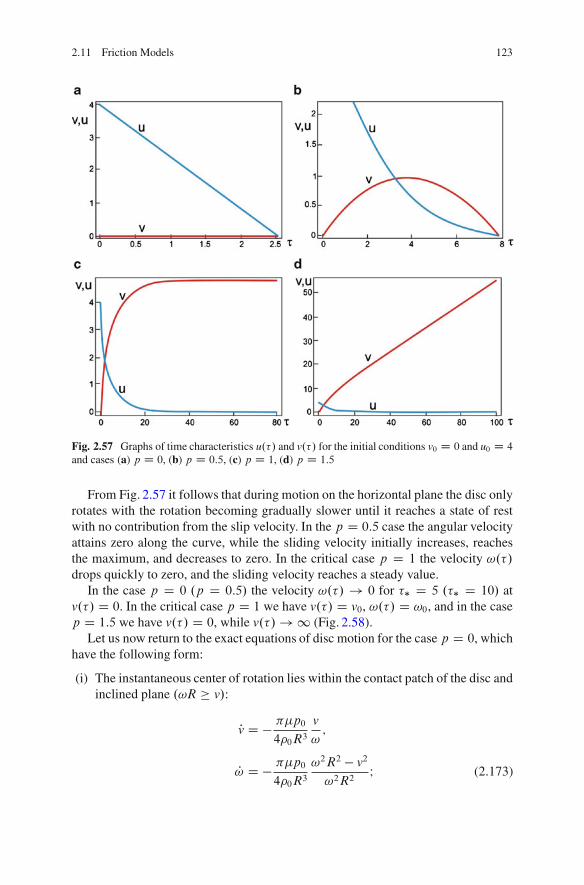
2.11 Friction Models 123
Fig. 2.57 Graphs of time characteristics u.�/ and v.�/ for the initial conditions v0 D 0 and u0 D 4
and cases (a) p D 0, (b) p D 0:5, (c) p D 1, (d) p D 1:5
From Fig. 2.57 it follows that during motion on the horizontal plane the disc onlyrotates with the rotation becoming gradually slower until it reaches a state of restwith no contribution from the slip velocity. In the p D 0:5 case the angular velocityattains zero along the curve, while the sliding velocity initially increases, reachesthe maximum, and decreases to zero. In the critical case p D 1 the velocity !.�/drops quickly to zero, and the sliding velocity reaches a steady value.
In the case p D 0 .p D 0:5/ the velocity !.�/ ! 0 for �� D 5 .�� D 10/ atv.�/ D 0. In the critical case p D 1 we have v.�/ D v0, !.�/ D !0, and in the casep D 1:5 we have v.�/ D 0, while v.�/ ! 1 (Fig. 2.58).
Let us now return to the exact equations of disc motion for the case p D 0, whichhave the following form:
(i) The instantaneous center of rotation lies within the contact patch of the disc andinclined plane .!R v/:
Pv D � ��p0
40R3v
!;
P! D � ��p0
40R3!2R2 � v2
!2R2I (2.173)
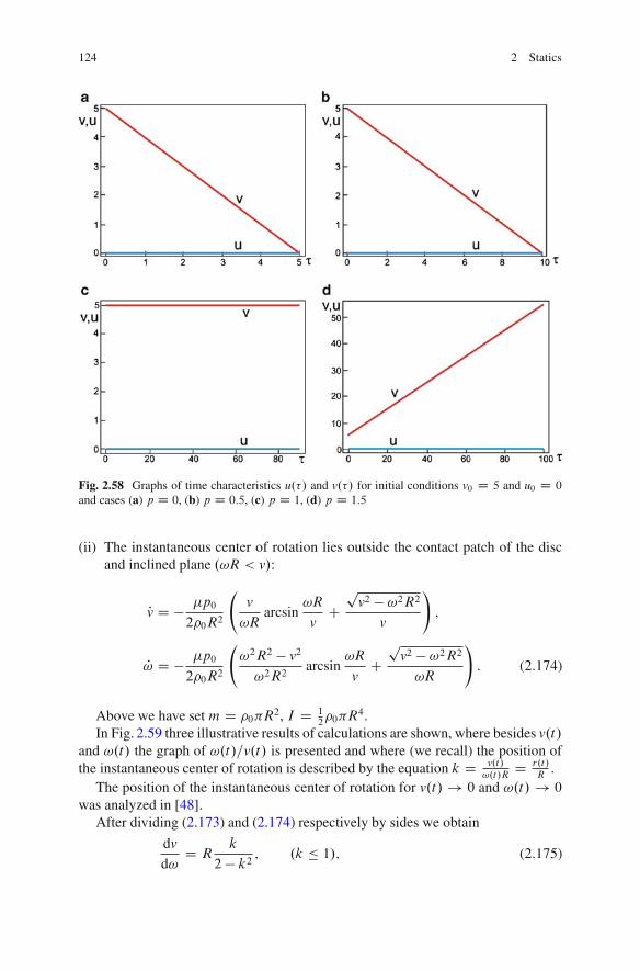
124 2 Statics
Fig. 2.58 Graphs of time characteristics u.�/ and v.�/ for initial conditions v0 D 5 and u0 D 0
and cases (a) p D 0, (b) p D 0:5, (c) p D 1, (d) p D 1:5
(ii) The instantaneous center of rotation lies outside the contact patch of the discand inclined plane .!R < v/:
Pv D � �p0
20R2
v
!Rarcsin
!R
vC
pv2 � !2R2
v
!;
P! D � �p0
20R2
!2R2 � v2
!2R2arcsin
!R
vC
pv2 � !2R2!R
!: (2.174)
Above we have set m D 0�R2, I D 1
20�R
4.In Fig. 2.59 three illustrative results of calculations are shown, where besides v.t/
and !.t/ the graph of !.t/=v.t/ is presented and where (we recall) the position ofthe instantaneous center of rotation is described by the equation k D v.t/
!.t/RD r.t/
R.
The position of the instantaneous center of rotation for v.t/ ! 0 and !.t/ ! 0
was analyzed in [48].After dividing (2.173) and (2.174) respectively by sides we obtain
dv
d!D R
k
2 � k2 ; .k � 1/; (2.175)
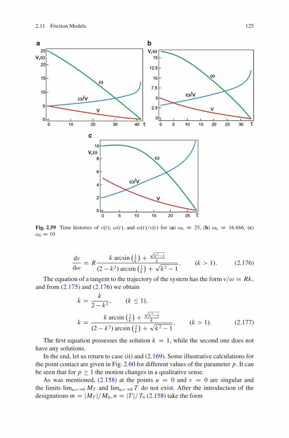
2.11 Friction Models 125
Fig. 2.59 Time histories of v.t /, !.t/, and !.t/=v.t / for (a) !0 D 25, (b) !0 D 16:666, (c)!0 D 10
dv
d!D R
k arcsin�1k
�Cpk2�1k
.2 � k2/ arcsin�1k
�C pk2 � 1 ; .k > 1/: (2.176)
The equation of a tangent to the trajectory of the system has the form v=! D Rk,and from (2.175) and (2.176) we obtain
k D k
2 � k2; .k � 1/;
k D k arcsin�1k
�Cpk2�1k
.2 � k2/ arcsin�1k
�C pk2 � 1
; .k > 1/: (2.177)
The first equation possesses the solution k D 1, while the second one does nothave any solutions.
In the end, let us return to case (ii) and (2.169). Some illustrative calculations forthe point contact are given in Fig. 2.60 for different values of the parameter p. It canbe seen that for p 1 the motion changes in a qualitative sense.
As was mentioned, (2.158) at the points u D 0 and v D 0 are singular andthe limits limu;v!0 MT and limu;v!0 T do not exist. After the introduction of thedesignationsm D jMT j=M0, n D jT j=T0 (2.158) take the form
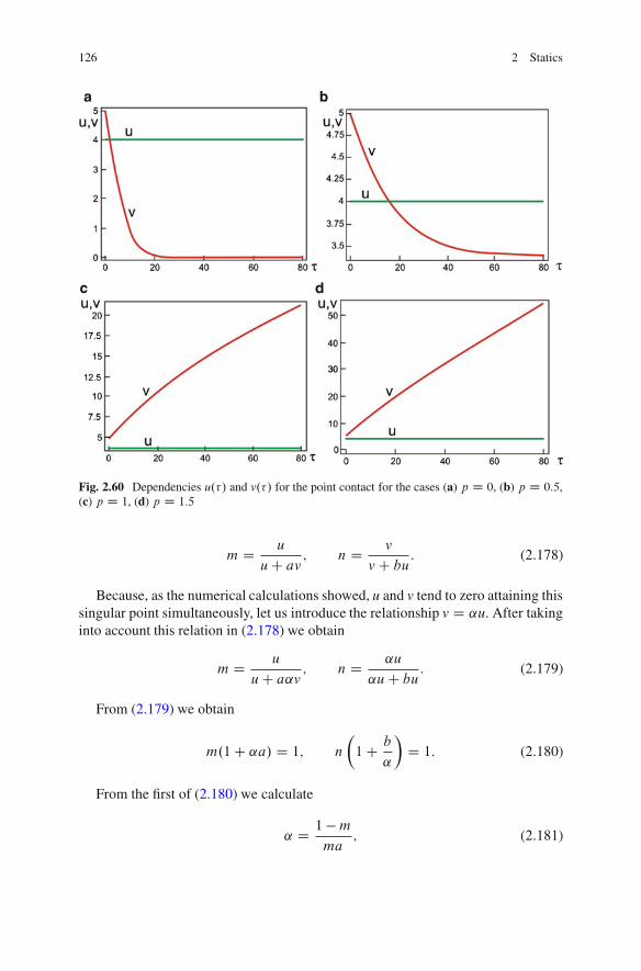
126 2 Statics
Fig. 2.60 Dependencies u.�/ and v.�/ for the point contact for the cases (a) p D 0, (b) p D 0:5,(c) p D 1, (d) p D 1:5
m D u
u C av; n D v
v C bu: (2.178)
Because, as the numerical calculations showed, u and v tend to zero attaining thissingular point simultaneously, let us introduce the relationship v D ˛u. After takinginto account this relation in (2.178) we obtain
m D u
u C a˛v; n D ˛u
˛u C bu: (2.179)
From (2.179) we obtain
m.1C ˛a/ D 1; n
1C b
˛
�D 1: (2.180)
From the first of (2.180) we calculate
˛ D 1 �mma
; (2.181)
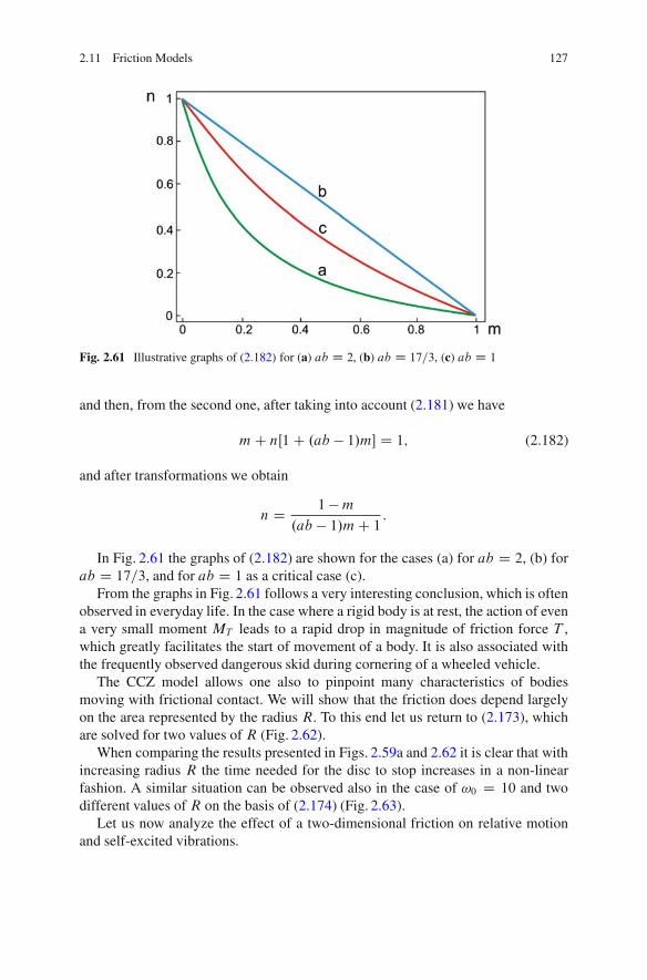
2.11 Friction Models 127
Fig. 2.61 Illustrative graphs of (2.182) for (a) ab D 2, (b) ab D 17=3, (c) ab D 1
and then, from the second one, after taking into account (2.181) we have
mC nŒ1C .ab � 1/m� D 1; (2.182)
and after transformations we obtain
n D 1 �m.ab � 1/mC 1
:
In Fig. 2.61 the graphs of (2.182) are shown for the cases (a) for ab D 2, (b) forab D 17=3, and for ab D 1 as a critical case (c).
From the graphs in Fig. 2.61 follows a very interesting conclusion, which is oftenobserved in everyday life. In the case where a rigid body is at rest, the action of evena very small moment MT leads to a rapid drop in magnitude of friction force T ,which greatly facilitates the start of movement of a body. It is also associated withthe frequently observed dangerous skid during cornering of a wheeled vehicle.
The CCZ model allows one also to pinpoint many characteristics of bodiesmoving with frictional contact. We will show that the friction does depend largelyon the area represented by the radius R. To this end let us return to (2.173), whichare solved for two values of R (Fig. 2.62).
When comparing the results presented in Figs. 2.59a and 2.62 it is clear that withincreasing radius R the time needed for the disc to stop increases in a non-linearfashion. A similar situation can be observed also in the case of !0 D 10 and twodifferent values of R on the basis of (2.174) (Fig. 2.63).
Let us now analyze the effect of a two-dimensional friction on relative motionand self-excited vibrations.
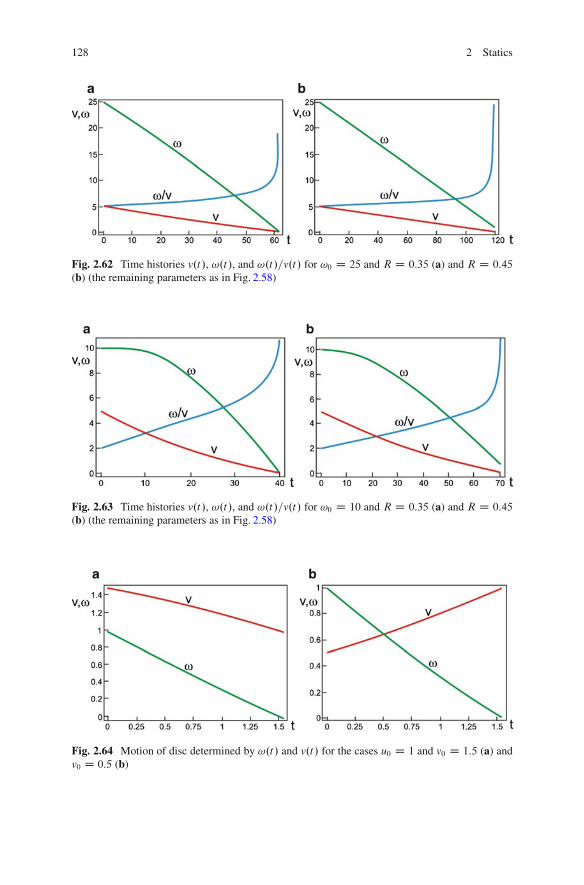
128 2 Statics
Fig. 2.62 Time histories v.t /, !.t/, and !.t/=v.t / for !0 D 25 and R D 0:35 (a) and R D 0:45
(b) (the remaining parameters as in Fig. 2.58)
Fig. 2.63 Time histories v.t /, !.t/, and !.t/=v.t / for !0 D 10 and R D 0:35 (a) and R D 0:45
(b) (the remaining parameters as in Fig. 2.58)
Fig. 2.64 Motion of disc determined by !.t/ and v.t / for the cases u0 D 1 and v0 D 1:5 (a) andv0 D 0:5 (b)
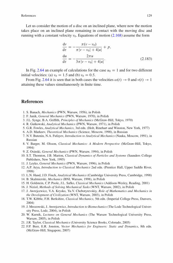
References 129
Let us consider the motion of a disc on an inclined plane, where now the motiontakes place on an inclined plane remaining in contact with the moving disc andrunning with a constant velocity v0. Equations of motion (2.168) assume the form
dv
d�D � �.v � v0/
�jv � v0j C 4juj C p;
du
d�D � 2�u
3�jv � v0j C 4juj : (2.183)
In Fig. 2.64 an example of calculations for the case u0 D 1 and for two differentinitial velocities: (a) v0 D 1:5 and (b) v0 D 0:5.
From Fig. 2.64 it is seen that in both cases the velocities !.t/ ! 0 and v.t/ ! 1
attaining these values simultaneously in finite time.
References
1. S. Banach, Mechanics (PWN, Warsaw, 1956), in Polish2. F. Janik, General Mechanics (PWN, Warsaw, 1970), in Polish3. J.L. Synge, B.A. Griffith, Principles of Mechanics (McGraw-Hill, Tokyo, 1970)4. R. Gutkowski, Analytical Mechanics (PWN, Warsaw, 1971), in Polish5. G.R. Fowles, Analytical Mechanics, 3rd edn. (Holt, Rinehart and Winston, New York, 1977)6. A.D. Markeev, Theoretical Mechanics (Science, Moscow, 1990), in Russian7. N.V. Butenin, N.A. Fufayev, Introduction to Analytical Mechanics (Nauka, Moscow, 1991), in
Russian8. V. Barger, M. Olsson, Classical Mechanics: A Modern Perspective (McGraw-Hill, Tokyo,
1994)9. Z. Osinski, General Mechanics (PWN, Warsaw, 1994), in Polish
10. S.T. Thornton, J.B. Marion, Classical Dynamics of Particles and Systems (Saunders CollegePublishers, New York, 1995)
11. J. Leyko, General Mechanics (PWN, Warsaw, 1996), in Polish12. A.P. Arya, Introduction to Classical Mechanics 2nd edn. (Prentice Hall, Upper Saddle River,
1998)13. L.N. Hand, J.D. Finch, Analytical Mechanics (Cambridge University Press, Cambridge, 1998)14. B. Skalmierski, Mechanics (BNI, Warsaw, 1998), in Polish15. H. Goldstein, C.P. Poole, J.L. Safko, Classical Mechanics (Addison-Wesley, Reading, 2001)16. J. Niziol, Methods of Solving Mechanical Tasks (WNT, Warsaw, 2002), in Polish17. J. Awrejcewicz, V.A. Krysko, Yu.V. Chebotyrevskiy, Role of Mathematics and Mechanics in
the Development of Civilization (WNT, Warsaw, 2003), in Polish18. T.W. Kibble, F.H. Berkshire, Classical Mechanics, 5th edn. (Imperial College Press, Danvers,
2004)19. J. Mrozowski, J. Awrejcewicz, Introduction to Biomechanics (The Lodz Technological Univer-
sity Press, Lodz, 2004), in Polish20. W. Kurnik, Lectures on General Mechanics (The Warsaw Technological University Press,
Warsaw, 2005), in Polish21. J.R. Taylor, Classical Mechanics (University Science Books, Colorado, 2005)22. F.P. Beer, E.R. Jonston, Vector Mechanics for Engineers: Static and Dynamics, 8th edn.
(McGraw-Hill, Singapore, 2007)
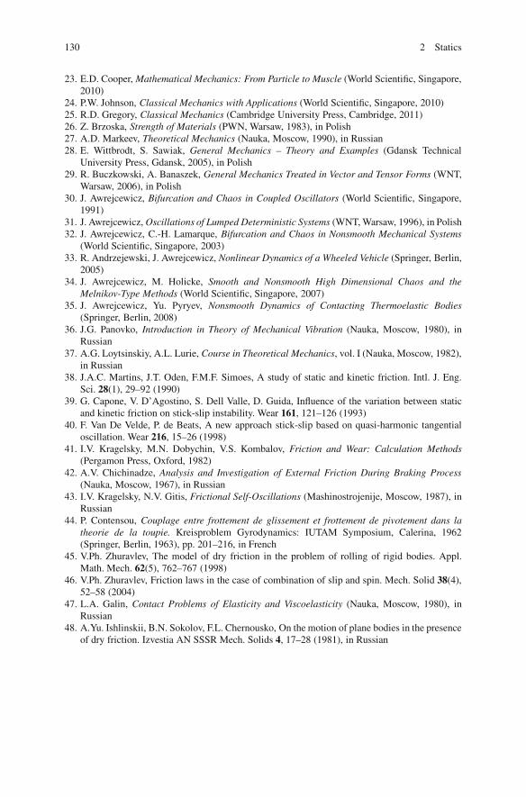
130 2 Statics
23. E.D. Cooper, Mathematical Mechanics: From Particle to Muscle (World Scientific, Singapore,2010)
24. P.W. Johnson, Classical Mechanics with Applications (World Scientific, Singapore, 2010)25. R.D. Gregory, Classical Mechanics (Cambridge University Press, Cambridge, 2011)26. Z. Brzoska, Strength of Materials (PWN, Warsaw, 1983), in Polish27. A.D. Markeev, Theoretical Mechanics (Nauka, Moscow, 1990), in Russian28. E. Wittbrodt, S. Sawiak, General Mechanics – Theory and Examples (Gdansk Technical
University Press, Gdansk, 2005), in Polish29. R. Buczkowski, A. Banaszek, General Mechanics Treated in Vector and Tensor Forms (WNT,
Warsaw, 2006), in Polish30. J. Awrejcewicz, Bifurcation and Chaos in Coupled Oscillators (World Scientific, Singapore,
1991)31. J. Awrejcewicz, Oscillations of Lumped Deterministic Systems (WNT, Warsaw, 1996), in Polish32. J. Awrejcewicz, C.-H. Lamarque, Bifurcation and Chaos in Nonsmooth Mechanical Systems
(World Scientific, Singapore, 2003)33. R. Andrzejewski, J. Awrejcewicz, Nonlinear Dynamics of a Wheeled Vehicle (Springer, Berlin,
2005)34. J. Awrejcewicz, M. Holicke, Smooth and Nonsmooth High Dimensional Chaos and the
Melnikov-Type Methods (World Scientific, Singapore, 2007)35. J. Awrejcewicz, Yu. Pyryev, Nonsmooth Dynamics of Contacting Thermoelastic Bodies
(Springer, Berlin, 2008)36. J.G. Panovko, Introduction in Theory of Mechanical Vibration (Nauka, Moscow, 1980), in
Russian37. A.G. Loytsinskiy, A.L. Lurie, Course in Theoretical Mechanics, vol. I (Nauka, Moscow, 1982),
in Russian38. J.A.C. Martins, J.T. Oden, F.M.F. Simoes, A study of static and kinetic friction. Intl. J. Eng.
Sci. 28(1), 29–92 (1990)39. G. Capone, V. D’Agostino, S. Dell Valle, D. Guida, Influence of the variation between static
and kinetic friction on stick-slip instability. Wear 161, 121–126 (1993)40. F. Van De Velde, P. de Beats, A new approach stick-slip based on quasi-harmonic tangential
oscillation. Wear 216, 15–26 (1998)41. I.V. Kragelsky, M.N. Dobychin, V.S. Kombalov, Friction and Wear: Calculation Methods
(Pergamon Press, Oxford, 1982)42. A.V. Chichinadze, Analysis and Investigation of External Friction During Braking Process
(Nauka, Moscow, 1967), in Russian43. I.V. Kragelsky, N.V. Gitis, Frictional Self-Oscillations (Mashinostrojenije, Moscow, 1987), in
Russian44. P. Contensou, Couplage entre frottement de glissement et frottement de pivotement dans la
theorie de la toupie. Kreisproblem Gyrodynamics: IUTAM Symposium, Calerina, 1962(Springer, Berlin, 1963), pp. 201–216, in French
45. V.Ph. Zhuravlev, The model of dry friction in the problem of rolling of rigid bodies. Appl.Math. Mech. 62(5), 762–767 (1998)
46. V.Ph. Zhuravlev, Friction laws in the case of combination of slip and spin. Mech. Solid 38(4),52–58 (2004)
47. L.A. Galin, Contact Problems of Elasticity and Viscoelasticity (Nauka, Moscow, 1980), inRussian
48. A.Yu. Ishlinskii, B.N. Sokolov, F.L. Chernousko, On the motion of plane bodies in the presenceof dry friction. Izvestia AN SSSR Mech. Solids 4, 17–28 (1981), in Russian

http://www.springer.com/978-1-4614-3790-1