Chapter 2 Paths and Searching - Department of …rg/book/chap2.pdf2 Chapter 2: Paths and Searching graph. We now have a very general and ﬂexible idea of distance that applies in

Chapter 2

Paths and Searching

Section 2.1 Distance

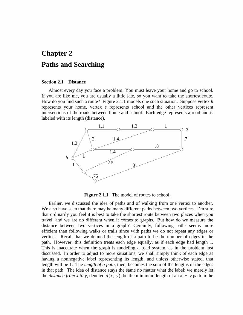
Almost every day you face a problem: You must leave your home and go to school.If you are like me, you are usually a little late, so you want to take the shortest route.How do you find such a route? Figure 2.1.1 models one such situation. Suppose vertex hrepresents your home, vertex s represents school and the other vertices representintersections of the roads between home and school. Each edge represents a road and islabeled with its length (distance).

1.2

1.1 1.2

.7

1

2 1.4

1

.75

11.4

.8

32.5h

s

Figure 2.1.1. The model of routes to school.

Earlier, we discussed the idea of paths and of walking from one vertex to another.We also have seen that there may be many different paths between two vertices. I’m surethat ordinarily you feel it is best to take the shortest route between two places when youtravel, and we are no different when it comes to graphs. But how do we measure thedistance between two vertices in a graph? Certainly, following paths seems moreefficient than following walks or trails since with paths we do not repeat any edges orvertices. Recall that we defined the length of a path to be the number of edges in thepath. However, this definition treats each edge equally, as if each edge had length 1.This is inaccurate when the graph is modeling a road system, as in the problem justdiscussed. In order to adjust to more situations, we shall simply think of each edge ashaving a nonnegative label representing its length, and unless otherwise stated, thatlength will be 1. The length of a path, then, becomes the sum of the lengths of the edgesin that path. The idea of distance stays the same no matter what the label; we merely letthe distance from x to y, denoted d(x , y), be the minimum length of an x − y path in the

2 Chapter 2: Paths and Searching

graph. We now have a very general and flexible idea of distance that applies in manysettings and is useful in many applications.

But how do we go about finding the distance between two vertices? What do we doto find the distance between all pairs of vertices? What properties does distance have?Does graph distance behave as one usually expects distance to behave? For that matter,how does one expect distance functions to behave? Let’s try to answer these questions.

We restrict the length of any edge to a positive number, since this corresponds to ourintuition of what length should be. In doing this, we can show that the followingproperties hold for the distance function d on a graph G (see exercises):

1. d(x , y) ≥ 0 and d(x , y) = 0 if, and only if, x = y.

2. d(x , y) = d(y , x).

3. d(x , y) + d(y , z) ≥ d(x , z).

These three properties define what is normally called a metric function (or simply ametric) on the vertex set of a graph. Metrics are well-behaved functions that reflect thethree properties usually felt to be fundamental to distance (namely, properties 1 − 3).Does each of these properties also hold for digraphs?

The diameter, denoted diam(G), of a connected graph G equalsu ∈ Vmax

v ∈ Vmax d(u , v),

while the radius of G, denoted rad(G), equalsu ∈ Vmin

v ∈ Vmax d(u , v). Theorem 2.1.1

shows that these terms are related in a manner that is also consistent with our intuitionabout distance.

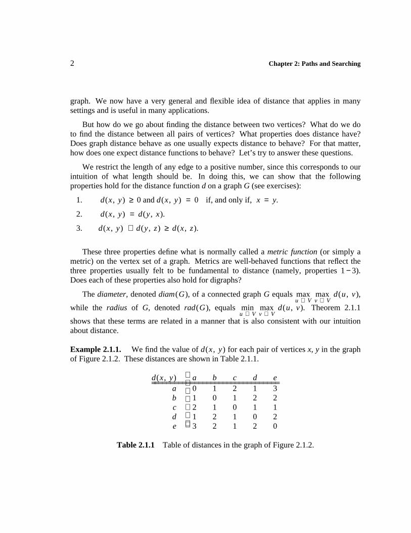
Example 2.1.1. We find the value of d(x , y) for each pair of vertices x, y in the graphof Figure 2.1.2. These distances are shown in Table 2.1.1.

d(x , y) a b c d e_ ________________________________ _______________________________a 0 1 2 1 3b 1 0 1 2 2c 2 1 0 1 1d 1 2 1 0 2e 3 2 1 2 0

Table 2.1.1 Table of distances in the graph of Figure 2.1.2.

Chapter 2: Paths and Searching 3

a

b

c

d

e

Figure 2.1.2. A graph of diameter 3 and radius 2.

Theorem 2.1.1 For any connected graph G,

rad(G) ≤ diam(G) ≤ 2rad(G) .

Proof. The first inequality comes directly from our definitions of radius and diameter.To prove the second inequality, let x , y ∈ V(G) such that d(x , y) = diam(G). Further,let z be chosen so that the longest distance path from z has length rad(G). Since distanceis a metric, by property (3) we have that

diam(G) = d(x , y) ≤ d(x , z) + d(z , y) ≤ 2 rad(G) .

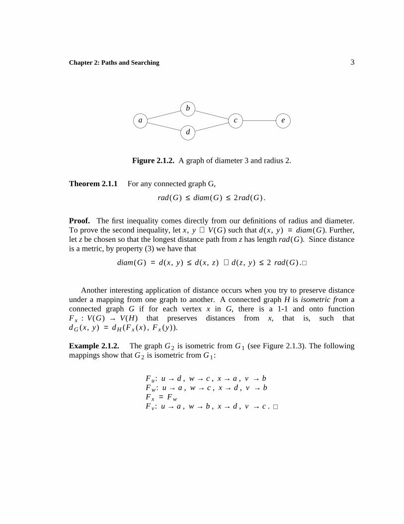
Another interesting application of distance occurs when you try to preserve distanceunder a mapping from one graph to another. A connected graph H is isometric from aconnected graph G if for each vertex x in G, there is a 1-1 and onto functionF x : V(G) → V(H) that preserves distances from x, that is, such thatd G (x , y) = d H (F x (x) , F x (y) ).

Example 2.1.2. The graph G 2 is isometric from G 1 (see Figure 2.1.3). The followingmappings show that G 2 is isometric from G 1:

F u: u → d , w → c , x → a , v → bF w: u → a , w → c , x → d , v → bF x = F wF v : u → a , w → b , x → d , v → c .


u v

w x

a b

c d

G 1: G 2:

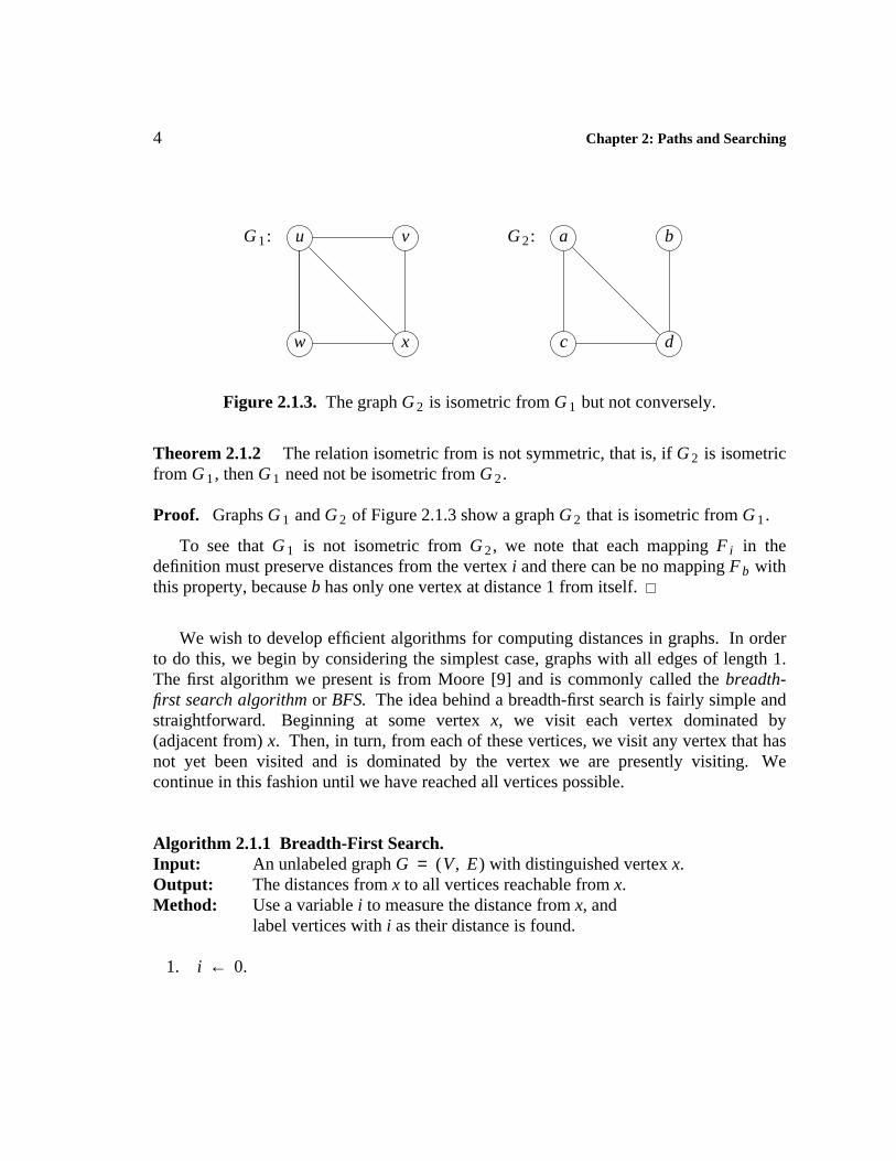
Figure 2.1.3. The graph G 2 is isometric from G 1 but not conversely.

Theorem 2.1.2 The relation isometric from is not symmetric, that is, if G 2 is isometricfrom G 1 , then G 1 need not be isometric from G 2 .

Proof. Graphs G 1 and G 2 of Figure 2.1.3 show a graph G 2 that is isometric from G 1 .

To see that G 1 is not isometric from G 2 , we note that each mapping F i in thedefinition must preserve distances from the vertex i and there can be no mapping F b withthis property, because b has only one vertex at distance 1 from itself.

We wish to develop efficient algorithms for computing distances in graphs. In orderto do this, we begin by considering the simplest case, graphs with all edges of length 1.The first algorithm we present is from Moore [9] and is commonly called the breadth-first search algorithm or BFS. The idea behind a breadth-first search is fairly simple andstraightforward. Beginning at some vertex x, we visit each vertex dominated by(adjacent from) x. Then, in turn, from each of these vertices, we visit any vertex that hasnot yet been visited and is dominated by the vertex we are presently visiting. Wecontinue in this fashion until we have reached all vertices possible.

Algorithm 2.1.1 Breadth-First Search.Input: An unlabeled graph G = (V , E) with distinguished vertex x.Output: The distances from x to all vertices reachable from x.Method: Use a variable i to measure the distance from x, and

label vertices with i as their distance is found.

1. i ← 0.


2. Label x with "i."

3. Find all unlabeled vertices adjacent to at least one vertex with label i. If none isfound, stop because we have reached all possible vertices.

4. Label all vertices found in step 3 with i + 1.

5. Let i ← i + 1, and go to step 3.

Example 2.1.3. As an example of the BFS algorithm, consider the graph of Figure2.1.2. If we begin our search at the vertex d, then the BFS algorithm will proceed asfollows:

1. Set i = 0.

2. Label d with 0.

3. Find all unlabeled vertices adjacent to d, namely a and c.

4. Label a and c with 1.

5. Set i = 1 and go to step 3.

3. Find all unlabeled vertices adjacent to one labeled 1, namely b and e.

4. Label b and e with 2.

5. Set i = 2 and go to step 3.

3. There are no unlabeled vertices adjacent to one labeled 2; hence, we stop.

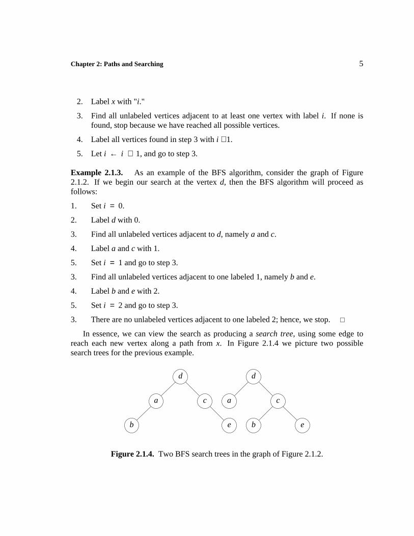
In essence, we can view the search as producing a search tree, using some edge toreach each new vertex along a path from x. In Figure 2.1.4 we picture two possiblesearch trees for the previous example.

d

a c

b e

d

a c

b e

Figure 2.1.4. Two BFS search trees in the graph of Figure 2.1.2.


Theorem 2.1.3 When the BFS algorithm halts, each vertex reachable from x is labeledwith its distance from x.

Proof. Suppose vertex v = v k has been labeled k. Then, by BFS (steps 3 and 4), theremust exist a vertex v k − 1 , which is labeled k − 1 and is adjacent to v k , and similarly avertex v k − 2 , which is labeled k − 2 and is adjacent to v k − 1 . By repeating thisargument, we eventually reach v 0 , and we see that v 0 = x, because x is the only vertexlabeled zero. Then

x = v 0 , v 1 , . . . , v k − 1 , v k = v

is a path of length k from x to v. Hence, d(x , v) ≤ k.

In order to prove that the label on v is the distance from x to v, we apply induction onk, the distance from x to v. In step 2 of BFS, we label x with 0, and clearly d(x , x) = 0.Now, assume the result holds for vertices with labels less than k and letP: x = v 0 , v 1 , . . . , v k = v be a shortest path from x to v in G. By the inductivehypothesis, v 0 , v 1 , . . . , v k − 1 is a shortest path from x to v k − 1 . By the inductivehypothesis, v k − 1 is labeled k − 1. By the algorithm, when i = k − 1, v receives thelabel k. To see that v could not have been labeled earlier, suppose that indeed it had beenlabeled with h < k. Then there would be an x − v path shorter than P, contradicting ourchoice of P. Hence, the result follows by induction.

When the BFS algorithm is performed, any edge in the graph is examined at most twotimes, once from each of its end vertices. Thus, in step 3 of the BFS algorithm, thevertices labeled i are examined for unvisited neighbors. Using incidence lists for thedata, the BFS algorithm has time complexity O(E). In order to obtain the distancesbetween any two vertices in the graph, we can perform the BFS algorithm, starting ateach vertex. Thus, to find all distances, the algorithm has time complexity O(V E).How does the BFS algorithm change for digraphs? Can you determine the timecomplexity for the directed version of BFS? Can you modify the BFS labeling process tomake it easier to find the x − v distance path?

Next, we want to consider arbitrarily labeled (sometimes these labels are calledweights) digraphs, that is, digraphs with arcs labeled l(e) ≥ 0. These labels couldrepresent the length of the arc e, as in our home to school example, or the cost oftraveling that route, or the cost of transmitting information between those locations, ortransmission times, or any of many other possibilities.

When we wish to determine the shortest path from vertex u to vertex v, it is clear thatwe must first gain information about distances to intermediate vertices. This information


is often recorded as a label assigned to the intermediate vertex. The label at intermediatevertex w usually takes one of two forms, the distance d(u , w) between u and w, orsometimes the pair d(u , w) and the predecessor of w on this path, pred(w). Thepredecessor aids in backtracking to find the actual path.

Many distance algorithms have been proposed and most can be classified as one oftwo types, based upon how many times the vertex labels are updated (see [6]). In label-setting methods, during each pass through the vertices, one vertex label is assigned avalue which remains unchanged thereafter. In label-correcting methods, any label maybe changed during processing. These methods have different limitations. Label-settingmethods cannot deal with graphs having negative arc labels. Label-correcting methodscan handle negative arc labels, provided no negative cycles exist, that is, a cycle withedge weight sum a negative value.

Most label-setting or correcting algorithms can be recast into the same basic formwhich allows for finding the shortest paths from one vertex to all other vertices. Oftenwhat distinguishes these algorithms is how they select the next vertex from the candidatelist C of vertices to examine. We now present a generic distance algorithm.

Algorithm 2.1.2a Generic Distance Algorithm.Input: A labeled digraph D = (V , E) with initial vertex v 1 .Output: The distance from v 1 to all other vertices.Method: Generic labeling of vertices with label (L(v) , pred(v) ).

1. For all v ∈ V(D) set L(v) ← ∞.

2. Initialize C = the set of vertices to be checked.

3. While C ≠ ∅;Select v ∈ C and set C = C − v.For all u adjacent from v;

If L(u) > L(v) + l(vu);L(u) = L(v) + l(vu);pred(u) = v;Add u to C if it is not there.

One of the earliest label-setting algorithms was given by Dijkstra [1]. In Dijkstra’salgorithm, a number of paths from vertex v 1 are tried and each time the shortest amongthem is chosen. Since paths can lead to new vertices with potentially many outgoingarcs, the number of paths can increase as we go. Each vertex is tried once, all pathsleading from it are added to the list and the vertex itself is labeled and no longer used(label-setting). After all vertices are visited the algorithm is finished. At any time during


execution of the algorithm, the value of L(v) attached to the vertex v is the length of theshortest v 1 − v path presently known.

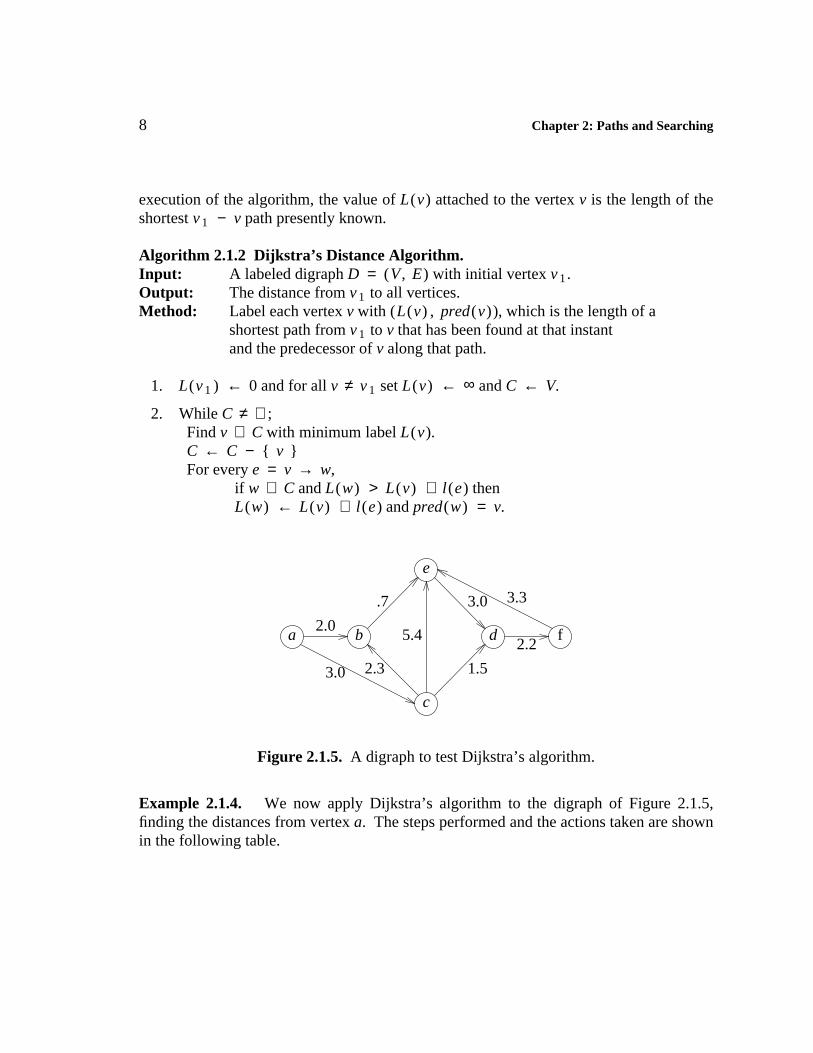
Algorithm 2.1.2 Dijkstra’s Distance Algorithm.Input: A labeled digraph D = (V , E) with initial vertex v 1 .Output: The distance from v 1 to all vertices.Method: Label each vertex v with (L(v) , pred(v) ), which is the length of a

shortest path from v 1 to v that has been found at that instantand the predecessor of v along that path.

1. L(v 1 ) ← 0 and for all v ≠ v 1 set L(v) ← ∞ and C ← V.

2. While C ≠ ∅;Find v ∈ C with minimum label L(v).C ← C − { v }For every e = v → w,

if w ∈ C and L(w) > L(v) + l(e) thenL(w) ← L(v) + l(e) and pred(w) = v.

a b

c

e

d f2.0

2.2

3.0.7

2.3 1.5

5.4

3.0

3.3

Figure 2.1.5. A digraph to test Dijkstra’s algorithm.

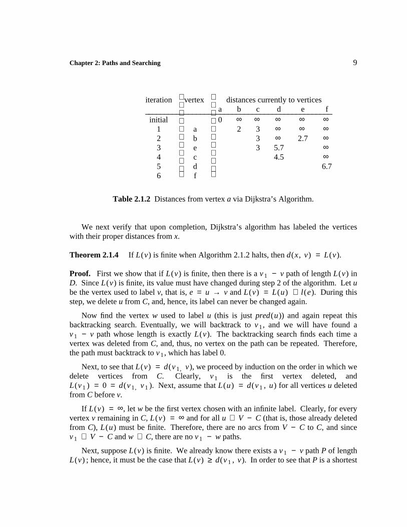
Example 2.1.4. We now apply Dijkstra’s algorithm to the digraph of Figure 2.1.5,finding the distances from vertex a. The steps performed and the actions taken are shownin the following table.


iteration vertex distances currently to verticesa b c d e f_ ______________________________________________

initial 0 ∞ ∞ ∞ ∞ ∞1 a 2 3 ∞ ∞ ∞2 b 3 ∞ 2.7 ∞3 e 3 5.7 ∞4 c 4.5 ∞5 d 6.76 f

Table 2.1.2 Distances from vertex a via Dijkstra’s Algorithm.

We next verify that upon completion, Dijkstra’s algorithm has labeled the verticeswith their proper distances from x.

Theorem 2.1.4 If L(v) is finite when Algorithm 2.1.2 halts, then d(x , v) = L(v).

Proof. First we show that if L(v) is finite, then there is a v 1 − v path of length L(v) inD. Since L(v) is finite, its value must have changed during step 2 of the algorithm. Let ube the vertex used to label v, that is, e = u → v and L(v) = L(u) + l(e). During thisstep, we delete u from C, and, hence, its label can never be changed again.

Now find the vertex w used to label u (this is just pred(u)) and again repeat thisbacktracking search. Eventually, we will backtrack to v 1 , and we will have found av 1 − v path whose length is exactly L(v). The backtracking search finds each time avertex was deleted from C, and, thus, no vertex on the path can be repeated. Therefore,the path must backtrack to v 1 , which has label 0.

Next, to see that L(v) = d(v 1 , v), we proceed by induction on the order in which wedelete vertices from C. Clearly, v 1 is the first vertex deleted, andL(v 1 ) = 0 = d(v 1 , v 1 ). Next, assume that L(u) = d(v 1 , u) for all vertices u deletedfrom C before v.

If L(v) = ∞, let w be the first vertex chosen with an infinite label. Clearly, for everyvertex v remaining in C, L(v) = ∞ and for all u ∈ V − C (that is, those already deletedfrom C), L(u) must be finite. Therefore, there are no arcs from V − C to C, and sincev 1 ∈ V − C and w ∈ C, there are no v 1 − w paths.

Next, suppose L(v) is finite. We already know there exists a v 1 − v path P of lengthL(v) ; hence, it must be the case that L(v) ≥ d(v 1 , v). In order to see that P is a shortest


path, suppose thatP 1 : v 1 , v 2 , . . . , v k = v

is a shortest v 1 − v path and let e i = v i → v i + 1 . Then

d(v 1 , v i ) =j = 1Σ

i − 1l(e j ).

Suppose v i is the vertex of highest subscript on P 1 deleted from C before v. By theinductive hypothesis

L(v i ) = d(v 1 , v i ) =j = 1Σ

i − 1l(e j ).

If v i + 1 ≠ v, then L(v i + 1 ) ≤ L(v i ) + l(e i ) after v i is deleted from C. Since step 2 canonly decrease labels, when v is chosen, L(v i + 1 ) still satisfies the inequality. Thus,

L(v i + 1 ) ≤ L(v i ) + l(e i )= d(v 1 , v i ) + l(e i )= d(v 1 , v i + 1 ) ≤ d(v 1 , v).

If d(v 1 , v) < L(v), then v should not have been chosen. If v i + 1 = v, the sameargument shows that L(v) ≤ d(v 1 , v), which completes the proof.

We now determine the time complexity of Dijkstra’s algorithm. Note that in step 2,the minimum label of C must be found. This can certainly be done in C − 1comparisons. Initially, C = V, and step 4 reduces C one vertex at a time. Thus, the

process is repeated Vtimes. The time required in step 2 is then on the order ofi = 1ΣV

i

and therefore is O(V2 ).

Step 2 uses each arc once at most, so it requires at most O(E) = O(V2 ) time.The entire algorithm thus has time complexity O(V2 ). If we want to obtain thedistance between any two vertices, we can use this algorithm once with each vertexplaying the role of the initial vertex x. This process requires O(V3 ) time.

Can you modify Dijkstra’s algorithm to work on undirected graphs?

What can we do to further generalize the problems we have been considering? Onepossibility is to relax our idea of what the edge labels represent. If we consider theselabels as representing some general value and not merely distance, then we can permitthese labels to be negative. We call these generalized labels weights, and we denote themas w(e). The "distance" between two vertices x and y will now correspond to theminimum sum of the edge weights along any x − y path.


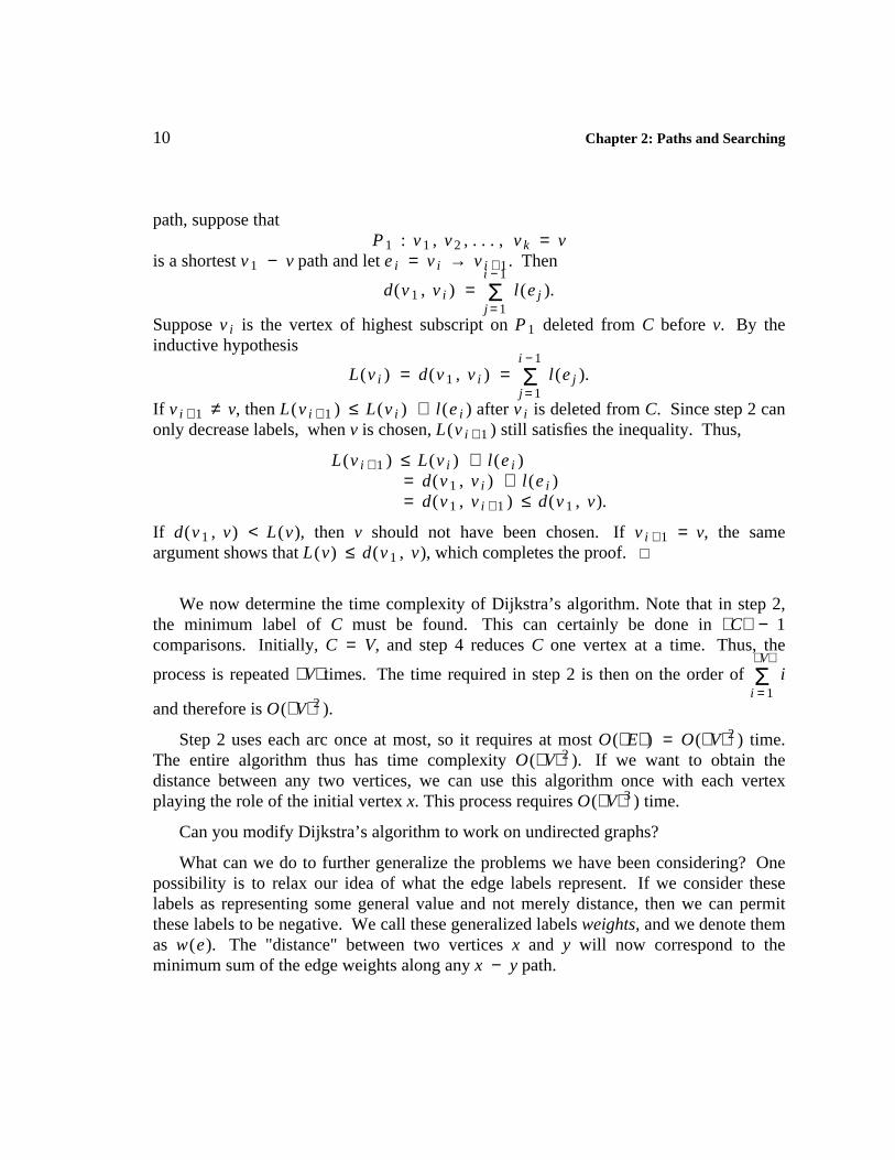
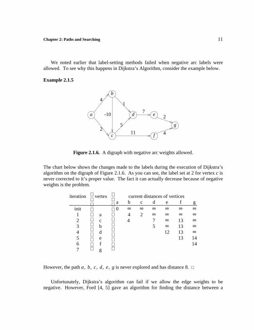
We noted earlier that label-setting methods failed when negative arc labels wereallowed. To see why this happens in Dijkstra’s Algorithm, consider the example below.

Example 2.1.5

a

b

c

d e

f

g

4

2

-10

1

5

7

11

2

4

Figure 2.1.6. A digraph with negative arc weights allowed.

The chart below shows the changes made to the labels during the execution of Dijkstra’salgorithm on the digraph of Figure 2.1.6. As you can see, the label set at 2 for vertex c isnever corrected to it’s proper value. The fact it can actually decrease because of negativeweights is the problem.

iteration vertex current distances of verticesa b c d e f g_ ___________________________________________________

init 0 ∞ ∞ ∞ ∞ ∞ ∞1 a 4 2 ∞ ∞ ∞ ∞2 c 4 7 ∞ 13 ∞3 b 5 ∞ 13 ∞4 d 12 13 ∞5 e 13 146 f 147 g

However, the path a , b , c , d , e , g is never explored and has distance 8.

Unfortunately, Dijkstra’s algorithm can fail if we allow the edge weights to benegative. However, Ford [4, 5] gave an algorithm for finding the distance between a


distinguished vertex x and all other vertices when we allow negative weights. Thisalgorithm features a label correcting method to record the distances found.

Initially, x is labeled 0 and every other vertex is labeled ∞. Ford’s algorithm, then,successively refines the labels assigned to the vertices, as long as improvements can bemade. Arcs are used to decrease the labels of the vertices they reach. There is a problem,however, when the digraph contains a cycle whose total length is negative (called anegative cycle). In this case, the algorithm continually traverses the negative cycle,decreasing the vertex labels and never halting. Thus, in order to properly use Ford’salgorithm, we must restrict its application to digraphs without negative cycles.

Algorithm 2.1.3 Ford’s Distance Algorithm.Input: A digraph with (possibly negative) arc weights w(e), but no

negative cycles.Output: The distance from x to all vertices reachable from x.Method: Label correcting.

1. L(x) ← 0 and for every v ≠ x set L(v) ← ∞.

2. While there is an arc e = u → v such that L(v) > L(u) + w(e)set L(v) ← L(u) + w(e) and pred(v) = u.

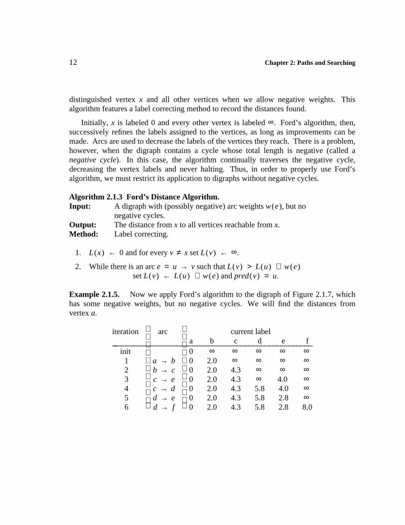
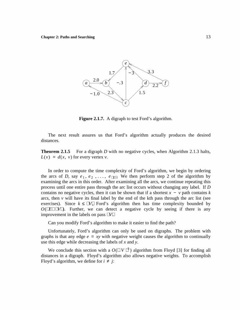
Example 2.1.5. Now we apply Ford’s algorithm to the digraph of Figure 2.1.7, whichhas some negative weights, but no negative cycles. We will find the distances fromvertex a.

iteration arc current labela b c d e f_ __________________________________________________

init 0 ∞ ∞ ∞ ∞ ∞1 a → b 0 2.0 ∞ ∞ ∞ ∞2 b → c 0 2.0 4.3 ∞ ∞ ∞3 c → e 0 2.0 4.3 ∞ 4.0 ∞4 c → d 0 2.0 4.3 5.8 4.0 ∞5 d → e 0 2.0 4.3 5.8 2.8 ∞6 d → f 0 2.0 4.3 5.8 2.8 8.0


a b

c

e

d f2.0

2.2

− 31.7

2.3 1. 5

−. 3

− 1. 0

3. 3

Figure 2.1.7. A digraph to test Ford’s algorithm.

The next result assures us that Ford’s algorithm actually produces the desireddistances.

Theorem 2.1.5 For a digraph D with no negative cycles, when Algorithm 2.1.3 halts,L(v) = d(x , v) for every vertex v.

In order to compute the time complexity of Ford’s algorithm, we begin by orderingthe arcs of D, say e 1 , e 2 , . . . , e E. We then perform step 2 of the algorithm byexamining the arcs in this order. After examining all the arcs, we continue repeating thisprocess until one entire pass through the arc list occurs without changing any label. If Dcontains no negative cycles, then it can be shown that if a shortest x − v path contains karcs, then v will have its final label by the end of the kth pass through the arc list (seeexercises). Since k ≤ V, Ford’s algorithm then has time complexity bounded byO(E V). Further, we can detect a negative cycle by seeing if there is anyimprovement in the labels on pass V.

Can you modify Ford’s algorithm to make it easier to find the path?

Unfortunately, Ford’s algorithm can only be used on digraphs. The problem withgraphs is that any edge e = xy with negative weight causes the algorithm to continuallyuse this edge while decreasing the labels of x and y.

We conclude this section with a O( V 3 ) algorithm from Floyd [3] for finding alldistances in a digraph. Floyd’s algorithm also allows negative weights. To accomplishFloyd’s algorithm, we define for i ≠ j:


d 0 (v i ,v j ) =∞l(e)

otherwise

if v i → v j

and let d k (v i ,v j ) be the length of a shortest path from v i to v j among all paths from v i tov j that use only vertices from the set { v 1 , v 2 , . . . , v k } . The distances are thenupdated as we allow the set of vertices used to build paths to expand. Thus, the d 0

distances represent the arcs of the digraph, the d 1 distances represent paths of length atmost two that include v 1 , etc. Note that because there are no negative cycles, thed k (v i , v i ) values will remain at 0.

Algorithm 2.1.4 Floyd’s Distance Algorithm.Input: A digraph D = (V , E) without negative cycles.Output: The distances from v i to v j .Method: Constant refinement of the distances as the set of excluded

vertices is decreased.

1. k ← 1.

2. For every 1 ≤ i, j ≤ n,d k (v i , v j ) ← min { d k − 1 (v i , v j ) , d k − 1 (v i , v k ) + d k − 1 (v k , v j ) }.

3. If k = V, then stop;else k ← k + 1 and go to 2.

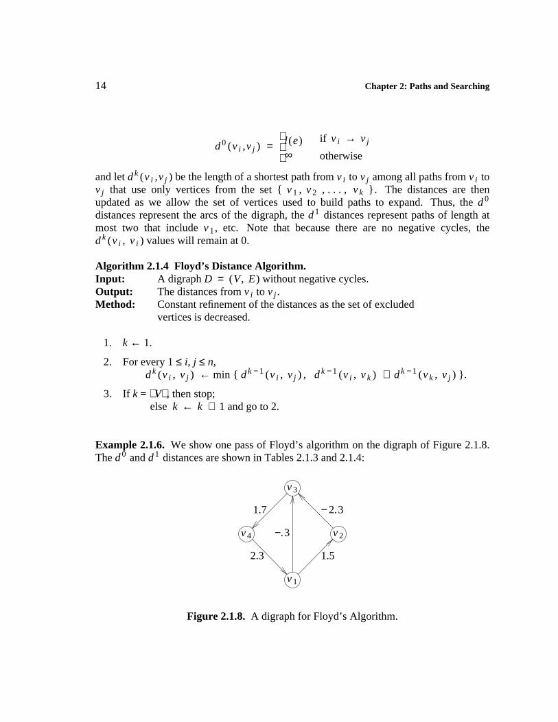
Example 2.1.6. We show one pass of Floyd’s algorithm on the digraph of Figure 2.1.8.The d 0 and d 1 distances are shown in Tables 2.1.3 and 2.1.4:

v 1

v 2

v 3

v 4

1.5

− 2. 31.7

2.3

−. 3

Figure 2.1.8. A digraph for Floyd’s Algorithm.


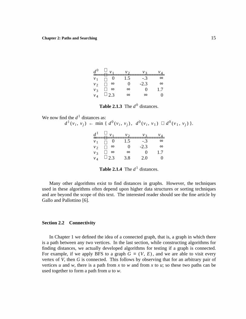
d 0 v 1 v 2 v 3 v 4_ ______________________________ _____________________________v 1 0 1.5 -.3 ∞v 2 ∞ 0 -2.3 ∞v 3 ∞ ∞ 0 1.7v 4 2.3 ∞ ∞ 0

Table 2.1.3 The d 0 distances.

We now find the d 1 distances as:d 1 (v i , v j ) ← min { d 0 (v i , v j ) , d 0 (v i , v 1 ) + d 0 (v 1 , v j ) }.

d 1 v 1 v 2 v 3 v 4_ ______________________________ _____________________________v 1 0 1.5 -.3 ∞v 2 ∞ 0 -2.3 ∞v 3 ∞ ∞ 0 1.7v 4 2.3 3.8 2.0 0

Table 2.1.4 The d 1 distances.

Many other algorithms exist to find distances in graphs. However, the techniquesused in these algorithms often depend upon higher data structures or sorting techniquesand are beyond the scope of this text. The interested reader should see the fine article byGallo and Pallottino [6].

Section 2.2 Connectivity

In Chapter 1 we defined the idea of a connected graph, that is, a graph in which thereis a path between any two vertices. In the last section, while constructing algorithms forfinding distances, we actually developed algorithms for testing if a graph is connected.For example, if we apply BFS to a graph G = (V , E) , and we are able to visit everyvertex of V, then G is connected. This follows by observing that for an arbitrary pair ofvertices u and w, there is a path from x to w and from x to u; so these two paths can beused together to form a path from u to w.


There are other techniques for determining if a graph is connected. Perhaps the bestknown of these is the approach of Tremaux [11] (see also [7]) known as the depth-firstsearch. The idea is to begin at a vertex v 0 and visit any vertex adjacent to v 0 , say v 1 .Now visit any vertex that is adjacent to v 1 that has not yet been visited. Continue toperform this process as long as possible. If we reach a vertex v k with the property that allits neighbors have been visited, we backtrack to the last vertex visited prior to going tov k , say v k − 1 . We then try to visit new vertices neighboring v k − 1 . If we can find anunvisited neighbor of v k − 1 , we visit it. If we cannot find such a vertex, we againbacktrack to the vertex visited immediately before v k − 1 , say v k − 2 . We continue visitingnew vertices where possible and backtracking where necessary until we backtrack to v 0and there are no unvisited neighbors at v 0 . At this stage we have visited all possiblevertices reachable from v 0 , and we stop.

The set of edges used in the depth-first search from v 0 are the edges of a tree. Uponreturning to v 0 , if we cannot continue the search and the graph still contains unvisitedvertices, we may choose such a vertex and begin the algorithm again. When all verticeshave been visited, the edges used in performing these visits are the edges of a forest(simply a tree when the graph is connected).

The depth-first search algorithm actually partitions the edge set into two sets T and B:those edges T contained in the forest (and, hence, used in the search), which are usuallycalled tree edges, and the remaining edges B = E − T, called back edges. The set B ofback edges can be further partitioned as follows: Let B 1 be the set of back edges that jointwo vertices x and y, along some path from v 0 to y in the depth-first search tree thatbegins at v 0 . Let C be the set of edges in B that join two vertices joined by a unique treepath that contains v 0 . The edges of C are called cross edges, since they are edgesbetween vertices that are not descendents of one another in the depth-first search tree.

Although it is not necessary in the search, we shall number the vertices v with aninteger n(v). The values of n(v) represent the order in which the vertices are firstencountered during the search. This numbering will be very useful in several problemsthat we will study later.

Algorithm 2.2.1 Depth-First Search.Input: A graph G = (V , E) and a distinguished vertex x.Output: A set T of tree edges and an ordering n(v) of the vertices.Method: Use a label m(e) to determine if an edge has been examined.

Use p(v) to record the vertex previous to v in the search.

1. For each e ∈ E, do the following: Set m(e) ← "unused."Set T ← ∅, i ← 0.


For every v ∈ V, do the following: set n(v) ← 0.

2. Let v ← x.

3. Let i ← i + 1 and let n(v) ← i.

4. If v has no unused incident edges, then go to 6.

5. Find an unused edge e = uv and set m(e) ← "used." Set T ← T ∪ { e } .If n(u) ≠ 0, then go to 4;

else p(u) ← v, v ← u and go to 3.

6. If n(v) = 1, then halt; else v ← p(v) and go to 4.

There is an alternate way of expressing recursive algorithms that often simplifies theirdescription. This method involves the use of procedures. The idea of a procedure is thatit is a "process" that can be repeatedly used in an algorithm. It is started with certainvalues, and the variables determined within the procedure are local to it. The proceduremay be halted at some stage by reference to another procedure or by reference to itself.Should this happen, another version of the procedure is invoked, with new parameterspassed to it, and all values of the old procedure are saved, until this procedure once againbegins its work. We now demonstrate such a procedural description of the depth-firstsearch algorithm.

Algorithm 2.2.2. Recursive Version of the Depth-First Search.Input: A graph G = (V , E) and a starting vertex v.Output: A set T of tree edges and an ordering of the vertices traversed.

1. Let i ← 1 and let F ← ∅. For all v ∈ V, do the following: Set n(v) ← 0.

2. While for some u, n(u) = 0, do the following: DFS(u).

3. Output T.

(The recursive procedure DFS is now given.)

Procedure DFS(v)

1. Let n(v) ← i and i ← i + 1.

2. For all u ∈ N(v), do the following:if n(u) = 0, then T ← T ∪ { e = uv }DFS(u)


end DFS

The depth-first search is an extremely important tool, with applications to many otheralgorithms. Often, an algorithm for determining a graph property or parameter isdependent on the structure of the particular graph under consideration, and we mustsearch that graph to discover this structural dependence. We shall have occasion to makeuse of the depth-first search as we continue to build other more complicated algorithms.

We now have a variety of ways of determining if a graph is connected. However,when dealing with graphs, you realize quickly that some graphs are "more connected"than others. For example, the path P n seems much less connected than the completegraph K n , in the sense that it is much easier to disconnect P n (remove one internal vertexor edge) than it is to disconnect K n (where removing a vertex merely reduces K n toK n − 1).

Denote by k(G) the connectivity of G, which is defined to be the minimum number ofvertices whose removal disconnects G or reduces it to a single vertex K 1 . Analogously,the edge connectivity, denoted k 1 (G), is the minimum number of edges whose removaldisconnects G. If G is disconnected, then k(G) = 0 = k 1 (G). If G = K n , thenk(G) = n − 1 = k 1 (G), as we must remove n − 1 vertices to reduce K n to K 1 , andwe can disconnect any vertex by removing the n − 1 edges incident with it.

We say G is n-connected if k(G) ≥ n and n-edge connected if k 1 (G) ≥ n. A set ofvertices whose removal increases the number of components in a graph is called a vertexseparating set (or vertex cut set) and a set of edges whose removal increases the numberof components in a graph is called an edge separating set (or edge cut set). If the contextis clear, we will simply use the term separating set (or cut set). If a cut set consists of asingle vertex, it is called a cut vertex (some call it an articulation point), while if the cutset consists of a single edge, this edge is called a cut-edge or bridge.

Paths can be used to describe both cut vertices and bridges.

Theorem 2.2.1 In a connected graph G:

1. A vertex v is a cut vertex if, and only if, there exist vertices u and w (u , w ≠ v)such that v is on every u − w path of G.

2. An edge e is a bridge if, and only if, there exist vertices u and w such that e is onevery u − w path of G.

Proof. To prove (1), let v be a cut vertex of G. If u and w are vertices in differentcomponents of G − v, then there are no u − w paths in G − v. However, since G is


connected, there are u − w paths in G. Thus, v must lie on every u − w path in G.

Conversely, suppose that there exist vertices u and w in G such that v lies on everyu − w in G. Then in G − v, there are no u − w paths, and so G − v is disconnected.Thus, v is a cut vertex of G.

To prove (2), let e be a bridge of G. Then G − e is disconnected. If u and w arevertices in different components of G − e, then there are no u − w paths in G − e. But,since G is connected, there are u − w paths in G. Thus, e must be on every u − w pathof G.

Conversely, if there exist vertices u and w such that e is on every u − w path in G,then clearly in G − e there are no u − w paths. Hence, G − e is disconnected, and,hence, e is a bridge.

The depth-first search algorithm can be modified to detect the blocks of a graph, thatis, the maximal 2-connected subgraphs. The strategy of the algorithm is based on thefollowing observations which are stated as a sequence of lemmas.

Lemma 2.2.1 Let G be a connected graph with DFS tree T. If vw is not a tree edge,then it is a back edge.

Lemma 2.2.2 For 1 ≤ i ≤ k, let G i = (V i , E i ) be the blocks of a connected graph G.Then

1. For all i ≠ j, V i ∩ V j contains at most one vertex.

2. Vertex x is a cut vertex if, and only if, x ∈ V i ∩ V j for some i ≠ j.

Lemma 2.2.3 Let G be a connected graph and T = (V , E 1 ) be a DFS search tree forG. Vertex x is a cut vertex of G if, and only if,

1. x is the root and x has more than one child in T, or

2. x is not the root and for some child s of x, there is no back edge between adescendant of s (including s itself) and a proper ancestor of x.

Suppose we perform a DFS on G and number the vertices n(v) as usual. Further,suppose we define a lowpoint function LP(v) as the minimum number of a vertexreachable from v by a path in T followed by at most one back edge. Then we can use thelowpoint function to help us determine cut vertices.


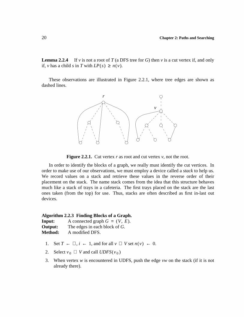
Lemma 2.2.4 If v is not a root of T (a DFS tree for G) then v is a cut vertex if, and onlyif, v has a child s in T with LP(s) ≥ n(v).

These observations are illustrated in Figure 2.2.1, where tree edges are shown asdashed lines.

r

v

Figure 2.2.1. Cut vertex r as root and cut vertex v, not the root.

In order to identify the blocks of a graph, we really must identify the cut vertices. Inorder to make use of our observations, we must employ a device called a stack to help us.We record values on a stack and retrieve these values in the reverse order of theirplacement on the stack. The name stack comes from the idea that this structure behavesmuch like a stack of trays in a cafeteria. The first trays placed on the stack are the lastones taken (from the top) for use. Thus, stacks are often described as first in-last outdevices.

Algorithm 2.2.3 Finding Blocks of a Graph.Input: A connected graph G = (V , E).Output: The edges in each block of G.Method: A modified DFS.

1. Set T ← ∅, i ← 1, and for all v ∈ V set n(v) ← 0.

2. Select v 0 ∈ V and call UDFS(v 0 )

3. When vertex w is encountered in UDFS, push the edge vw on the stack (if it is notalready there).


4. After discovering a pair vw such that w is a child of v and LP(w) ≥ n(v), popfrom the stack all edges up to and including vw. These are the edges from a blockof G

Upgraded DFS - Procedure UDFS(v)

1. i ← 1

2. n(v) ← i, LP(v) ← n(v) , i ← i + 1.

3. For all w ∈ N(v) , do the following:If n(w) = 0, then

add uv to Tp(w) ← vUDFS(w)If LP(w) ≥ n(v), then a block has been found.LP(v) ← min (LP(v) , LP(w) )

Else If w ≠ p(v), thenLP(v) ← min (LP(v) , n(w) )

A simple inequality from Whitney [12] relates connectivity, edge connectivity andthe minimum degree of a graph.

Theorem 2.2.2 For any graph G, k(G) ≤ k 1 (G) ≤ δ(G).

Proof. If G is disconnected, then clearly k 1 (G) = 0. If G is connected, we cancertainly disconnect it by removing all edges incident with a vertex of minimum degree.Thus, in either case, k 1 (G) ≤ δ(G).

To verify that the first inequality holds, note that if G is disconnected or trivial, thenclearly k(G) = k 1 (G) = 0. If G is connected and has a bridge, thenk 1 (G) = 1 = k(G), as either G = K 2 or G is connected and contains cut vertices.Finally, if k 1 (G) ≥ 2, then the removal of k 1 (G) − 1 of the edges in an edge-separating set leaves a graph that contains a bridge. Let this bridge be e = uv. For eachof the other edges, select an end vertex other than u or v and remove it from G. If theresulting graph is disconnected, then k(G) < k 1 (G). If the graph is connected, then itcontains the bridge e and the removal of either u or v disconnects it. In either case,k(G) ≤ k 1 (G), and the result is verified.


Can you find a graph G for which k(G) < k 1 (G) < δ(G)?

Bridges played an important role in the last proof. We can characterize bridges, againtaking a structural view using cycles.

Theorem 2.2.3 In a graph G, the edge e is a bridge if, and only if, e lies on no cycle ofG.

Proof. Assume G is connected and let e = uv be an edge of G. Suppose e lies on acycle C of G. Also let w 1 and w 2 be distinct arbitrary vertices of G. If e does not lie ona w 1 − w 2 path P, then P is also a w 1 − w 2 path in G − e. If e does lie on aw 1 − w 2 path P ′, then by replacing e by the u − v (or v − u) path of C not containing eproduces a w 1 − w 2 walk in G − e. Thus, there is a w 1 − w 2 path in G − e andhence, e is not a bridge.

Conversely, suppose e = uv is an edge of G that is on no cycle of G. Assume e isnot a bridge. Then, G − e is connected and hence there exists a u − v path P in G − e.Then P together with the edge e produces a cycle in G containing e, a contradiction.

With the aid of Theorem 2.2.3, we can now characterize 2-connected graphs. Onceagain cycles play a fundamental role in the characterization. Before presenting the result,we need another definition. Two u − v paths P 1 and P 2 are said to be internally disjointif

V(P 1 ) ∩ V(P 2 ) = { u , v }.

Theorem 2.2.4 (Whitney [12]). A graph G of order p ≥ 3 is 2-connected if, and onlyif, any two vertices of G lie on a common cycle.

Proof. If any two vertices of G lie on a common cycle, then clearly there are at leasttwo internally disjoint paths between these vertices. Thus, the removal of one vertexcannot disconnect G, that is, G is 2-connected.

Conversely, let G be a 2-connected graph. We use induction on d(u , v) to prove thatany two vertices u and v must lie on a common cycle.

If d(u , v) = 1, then since G is 2-connected, the edge uv is not a bridge. Hence, byTheorem 2.2.3, the edge uv lies on a cycle. Now, assume the result holds for any twovertices at a distance less than d in G and consider vertices u and v such thatd(u , v) = d ≥ 2. Let P be a u − v path of length d in G and suppose w precedes v onP. Since d(u , w) = d − 1, the induction hypothesis implies that u and w lie on a


common cycle, say C.

Since G is 2-connected, G − w is connected and, hence, contains a u − v path P 1 .Let z (possibly z = u) be the last vertex of P 1 on C. Since u ∈ V(C), such a vertexmust exist. Then G has two internally disjoint paths: one composed of the section of Cfrom u to z not containing w together with the section of P 1 from z to v, and the othercomposed of the other section of C from u to w together with the edge wv. These twopaths thus form a cycle containing u and v.

A very powerful generalization of Whitney’s theorem was proved by Menger [8].Menger’s theorem turns out to be related to many other results in several branches ofdiscrete mathematics. We shall see some of these relationships later. Although a proofof Menger’s theorem could be presented now, we postpone it until Chapter 4 in order tobetter point out some of these relationships to other results.

Theorem 2.2.5 (Menger’s theorem). For nonadjacent vertices u and v in a graph G,the maximum number of internally disjoint u − v paths equals the minimum number ofvertices that separate u and v.

Theorem 2.2.4 has a generalization (Whitney [12]) to the k-connected case. Thisresult should be viewed as the global version of Menger’s theorem.

Theorem 2.2.6 A graph G is k-connected if, and only if, all distinct pairs of verticesare joined by at least k internally disjoint paths.

It is natural to ask if there is an edge analog to Menger’s theorem. This result wasindependently discovered much later by Ford and Fulkerson [5] and Elias, Feinstein andShannon [2]. We postpone the proof of this result until Chapter 4.

Theorem 2.2.7 For any two vertices u and v of a graph G, the maximum number ofedge disjoint paths joining u and v equals the minimum number of edges whose removalseparates u and v.


Section 2.3 Digraph Connectivity

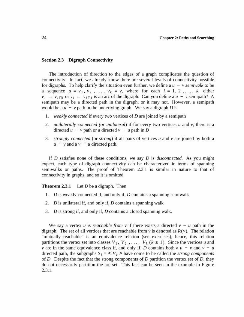
The introduction of direction to the edges of a graph complicates the question ofconnectivity. In fact, we already know there are several levels of connectivity possiblefor digraphs. To help clarify the situation even further, we define a u − v semiwalk to bea sequence u = v 1 , v 2 , . . . , v k = v, where for each i = 1 , 2 , . . . , k, eitherv i → v i + 1 or v i ← v i + 1 is an arc of the digraph. Can you define a u − v semipath? Asemipath may be a directed path in the digraph, or it may not. However, a semipathwould be a u − v path in the underlying graph. We say a digraph D is

1. weakly connected if every two vertices of D are joined by a semipath

2. unilaterally connected (or unilateral) if for every two vertices u and v, there is adirected u − v path or a directed v − u path in D

3. strongly connected (or strong) if all pairs of vertices u and v are joined by both au − v and a v − u directed path.

If D satisfies none of these conditions, we say D is disconnected. As you mightexpect, each type of digraph connectivity can be characterized in terms of spanningsemiwalks or paths. The proof of Theorem 2.3.1 is similar in nature to that ofconnectivity in graphs, and so it is omitted.

Theorem 2.3.1 Let D be a digraph. Then

1. D is weakly connected if, and only if, D contains a spanning semiwalk

2. D is unilateral if, and only if, D contains a spanning walk

3. D is strong if, and only if, D contains a closed spanning walk.

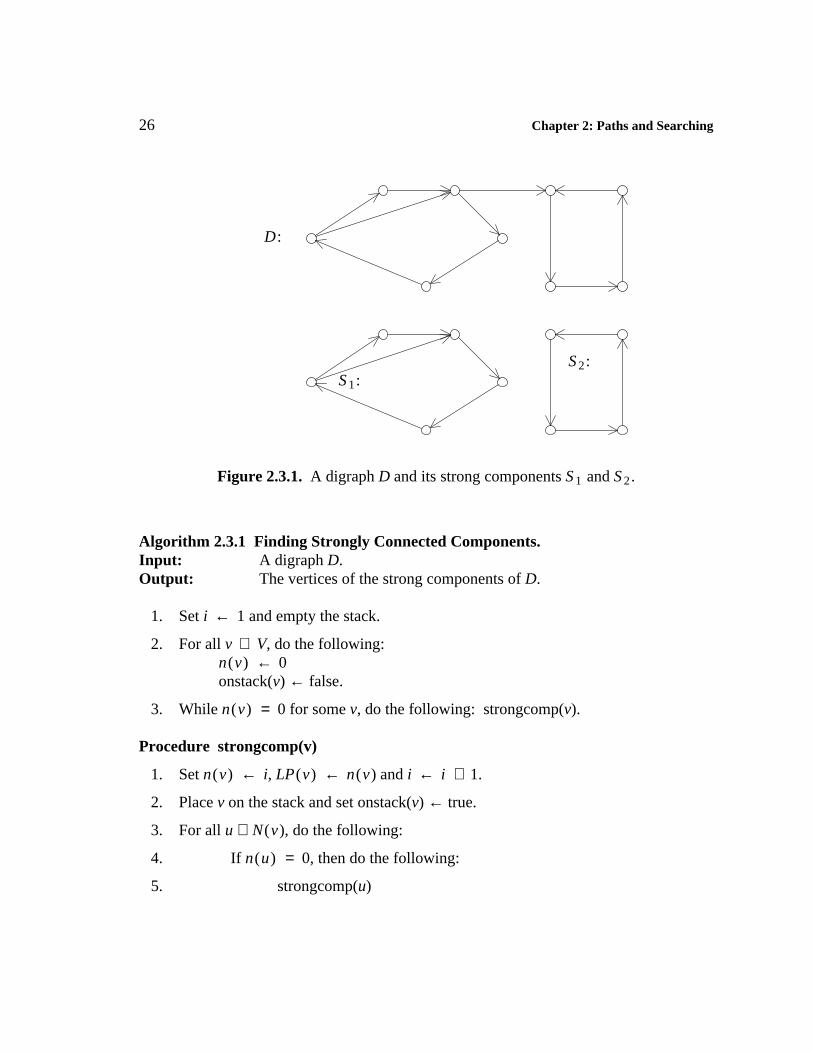
We say a vertex u is reachable from v if there exists a directed v − u path in thedigraph. The set of all vertices that are reachable from v is denoted as R(v). The relation"mutually reachable" is an equivalence relation (see exercises); hence, this relationpartitions the vertex set into classes V 1 , V 2 , . . . , V k (k ≥ 1 ). Since the vertices u andv are in the same equivalence class if, and only if, D contains both a u − v and v − udirected path, the subgraphs S i = < V i > have come to be called the strong componentsof D. Despite the fact that the strong components of D partition the vertex set of D, theydo not necessarily partition the arc set. This fact can be seen in the example in Figure2.3.1.


The term strong component is still appropriate, even when D is weakly connected orunilateral, since if S 1 and S 2 are two strong components, all arcs between these strongcomponents are directed in one way, from S 1 to S 2 or from S 2 to S 1 . Thus, there willalways be vertices in one of these components that cannot reach any vertex of the othercomponent.

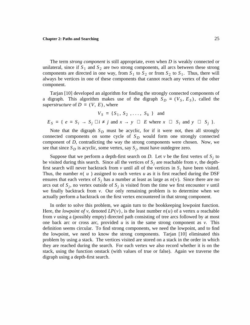
Tarjan [10] developed an algorithm for finding the strongly connected components ofa digraph. This algorithm makes use of the digraph S D = (V S , E S ) , called thesuperstructure of D = (V , E) , where

V S = {S 1 , S 2 , . . . , S k } and

E S = { e = S i → S j i ≠ j and x → y ∈ E where x ∈ S i and y ∈ S j }.

Note that the digraph S D must be acyclic, for if it were not, then all stronglyconnected components on some cycle of S D would form one strongly connectedcomponent of D, contradicting the way the strong components were chosen. Now, wesee that since S D is acyclic, some vertex, say S j , must have outdegree zero.

Suppose that we perform a depth-first search on D. Let v be the first vertex of S j tobe visited during this search. Since all the vertices of S j are reachable from v, the depth-first search will never backtrack from v until all of the vertices in S j have been visited.Thus, the number n( u ) assigned to each vertex u as it is first reached during the DSFensures that each vertex of S j has a number at least as large as n(v). Since there are noarcs out of S j , no vertex outside of S j is visited from the time we first encounter v untilwe finally backtrack from v. Our only remaining problem is to determine when weactually perform a backtrack on the first vertex encountered in that strong component.

In order to solve this problem, we again turn to the bookkeeping lowpoint function.Here, the lowpoint of v, denoted LP(v) , is the least number n(u) of a vertex u reachablefrom v using a (possibly empty) directed path consisting of tree arcs followed by at mostone back arc or cross arc, provided u is in the same strong component as v. Thisdefinition seems circular. To find strong components, we need the lowpoint, and to findthe lowpoint, we need to know the strong components. Tarjan [10] eliminated thisproblem by using a stack. The vertices visited are stored on a stack in the order in whichthey are reached during the search. For each vertex we also record whether it is on thestack, using the function onstack (with values of true or false). Again we traverse thedigraph using a depth-first search.


D:

S 1:S 2:

Figure 2.3.1. A digraph D and its strong components S 1 and S 2 .

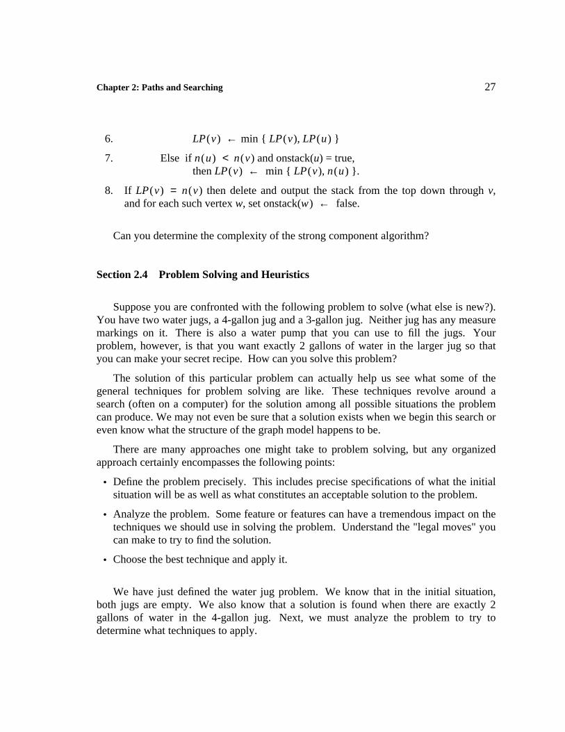
Algorithm 2.3.1 Finding Strongly Connected Components.Input: A digraph D.Output: The vertices of the strong components of D.

1. Set i ← 1 and empty the stack.

2. For all v ∈ V, do the following:n(v) ← 0onstack(v) ← false.

3. While n(v) = 0 for some v, do the following: strongcomp(v).

Procedure strongcomp(v)

1. Set n(v) ← i, LP(v) ← n(v) and i ← i + 1.

2. Place v on the stack and set onstack(v) ← true.

3. For all u ∈ N(v), do the following:

4. If n(u) = 0, then do the following:

5. strongcomp(u)


6. LP(v) ← min { LP(v), LP(u) }

7. Else if n(u) < n(v) and onstack(u) = true,then LP(v) ← min { LP(v), n(u) }.

8. If LP(v) = n(v) then delete and output the stack from the top down through v,and for each such vertex w, set onstack(w) ← false.

Can you determine the complexity of the strong component algorithm?

Section 2.4 Problem Solving and Heuristics

Suppose you are confronted with the following problem to solve (what else is new?).You have two water jugs, a 4-gallon jug and a 3-gallon jug. Neither jug has any measuremarkings on it. There is also a water pump that you can use to fill the jugs. Yourproblem, however, is that you want exactly 2 gallons of water in the larger jug so thatyou can make your secret recipe. How can you solve this problem?

The solution of this particular problem can actually help us see what some of thegeneral techniques for problem solving are like. These techniques revolve around asearch (often on a computer) for the solution among all possible situations the problemcan produce. We may not even be sure that a solution exists when we begin this search oreven know what the structure of the graph model happens to be.

There are many approaches one might take to problem solving, but any organizedapproach certainly encompasses the following points:

• Define the problem precisely. This includes precise specifications of what the initialsituation will be as well as what constitutes an acceptable solution to the problem.

• Analyze the problem. Some feature or features can have a tremendous impact on thetechniques we should use in solving the problem. Understand the "legal moves" youcan make to try to find the solution.

• Choose the best technique and apply it.

We have just defined the water jug problem. We know that in the initial situation,both jugs are empty. We also know that a solution is found when there are exactly 2gallons of water in the 4-gallon jug. Next, we must analyze the problem to try todetermine what techniques to apply.


We can perform several "legal" operations with the water jugs:

• We can fill either jug completely from the pump.

• We can pour all the water from one jug into the other jug.

• We can fill one jug from the other jug.

• We can dump all the water from either jug.

Why have we restricted our operations in these ways? The answer is so that we canmaintain control over the situation. By restricting operations in this way, we will alwaysknow exactly how much water is in either jug at any given time. Note that theseoperations also ensure that our search must deal with only a finite number of situations,since each jug can be filled to only a finite number of levels.

We have just examined an important concept, the idea of "moving" from onesituation to another by performing one of a set of legal moves. What we want to do is tomove from our present state (the starting vertex in the state space model) to some otherstate via these legal moves. Just what constitutes a legal move is dependent on theproblem at hand and should be the result of our problem analysis.

The digraph model we have been building should now be apparent. Represent eachstate that we can reach by a vertex. There is an arc from vertex a to vertex b if we canmove from state a to state b via some legal move. Our digraph and the collection of legalmoves that define its arcs, constitute the state space (or the state graph) of the problem.Let’s determine the state space of the water jug problem.

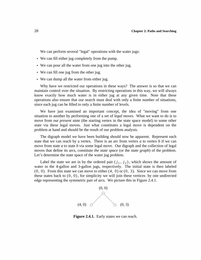
Label the state we are in by the ordered pair ( j 1 , j 2 ) , which shows the amount ofwater in the 4-gallon and 3-gallon jugs, respectively. The initial state is then labeled( 0 , 0 ). From this state we can move to either ( 4 , 0 ) or ( 0 , 3 ). Since we can move fromthese states back to ( 0 , 0 ) , for simplicity we will join these vertices by one undirectededge representing the symmetric pair of arcs. We picture this in Figure 2.4.1.

(0, 0)

(4, 0) (0, 3)

Figure 2.4.1. Early states we can reach.


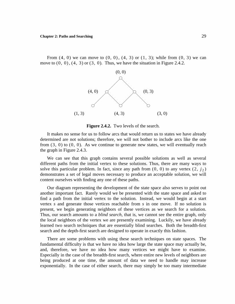
From ( 4 , 0 ) we can move to ( 0 , 0 ) , ( 4 , 3 ) or ( 1 , 3 ); while from ( 0 , 3 ) we canmove to ( 0 , 0 ) , ( 4 , 3 ) or ( 3 , 0 ). Thus, we have the situation in Figure 2.4.2.

(0, 0)

(4, 0) (0, 3)

(1, 3) (4, 3) (3, 0)

Figure 2.4.2. Two levels of the search.

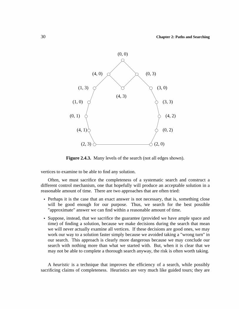
It makes no sense for us to follow arcs that would return us to states we have alreadydetermined are not solutions; therefore, we will not bother to include arcs like the onefrom ( 3 , 0 ) to ( 0 , 0 ). As we continue to generate new states, we will eventually reachthe graph in Figure 2.4.3.

We can see that this graph contains several possible solutions as well as severaldifferent paths from the initial vertex to these solutions. Thus, there are many ways tosolve this particular problem. In fact, since any path from ( 0 , 0 ) to any vertex ( 2 , j 2 )demonstrates a set of legal moves necessary to produce an acceptable solution, we willcontent ourselves with finding any one of these paths.

Our diagram representing the development of the state space also serves to point outanother important fact. Rarely would we be presented with the state space and asked tofind a path from the initial vertex to the solution. Instead, we would begin at a startvertex s and generate those vertices reachable from s in one move. If no solution ispresent, we begin generating neighbors of these vertices as we search for a solution.Thus, our search amounts to a blind search, that is, we cannot see the entire graph, onlythe local neighbors of the vertex we are presently examining. Luckily, we have alreadylearned two search techniques that are essentially blind searches. Both the breadth-firstsearch and the depth-first search are designed to operate in exactly this fashion.

There are some problems with using these search techniques on state spaces. Thefundamental difficulty is that we have no idea how large the state space may actually be,and, therefore, we have no idea how many vertices we might have to examine.Especially in the case of the breadth-first search, where entire new levels of neighbors arebeing produced at one time, the amount of data we need to handle may increaseexponentially. In the case of either search, there may simply be too many intermediate


(0, 0)

(4, 0) (0, 3)

(1, 3)

(4, 3)

(3, 0)

(1, 0)

(0, 1)

(4, 1)

(3, 3)

(4, 2)

(0, 2)

(2, 3) (2, 0)

Figure 2.4.3. Many levels of the search (not all edges shown).

vertices to examine to be able to find any solution.

Often, we must sacrifice the completeness of a systematic search and construct adifferent control mechanism, one that hopefully will produce an acceptable solution in areasonable amount of time. There are two approaches that are often tried:

• Perhaps it is the case that an exact answer is not necessary, that is, something closewill be good enough for our purpose. Thus, we search for the best possible"approximate" answer we can find within a reasonable amount of time.

• Suppose, instead, that we sacrifice the guarantee (provided we have ample space andtime) of finding a solution, because we make decisions during the search that meanwe will never actually examine all vertices. If these decisions are good ones, we maywork our way to a solution faster simply because we avoided taking a "wrong turn" inour search. This approach is clearly more dangerous because we may conclude oursearch with nothing more than what we started with. But, when it is clear that wemay not be able to complete a thorough search anyway, the risk is often worth taking.

A heuristic is a technique that improves the efficiency of a search, while possiblysacrificing claims of completeness. Heuristics are very much like guided tours; they are


intended to point out the highlights and eliminate time wasted on unnecessary events.Some heuristics are of more help than others, and usually this is a problem-dependentcharacteristic. However, several general heuristic techniques have become popular.

One general technique is called the nearest neighbor algorithm. The idea is that weexamine all unvisited neighbors of some vertex and next visit the neighbor that mostsatisfies some test criterion. Our hope is that the test criterion will point us more rapidlytoward a solution.

For example, suppose we apply the following heuristic to the water jug problem:During a DFS search we shall next visit the neighboring vertex whose label ( j 1 , j 2 ) hasj 1 closest to the desired value of two. Under these conditions our search would proceedas follows:

• From ( 0 , 0 ) we generate ( 4 , 0 ) and ( 0 , 3 ). Since either has first coordinate withintwo of the goal, we randomly select the first as our next state.

• From ( 4 , 0 ) we generate the neighbors ( 1 , 3 ) and ( 4 , 3 ), and since ( 1 , 3 ) is best,we move there.

• From ( 1 , 3 ) we generate in turn (as there is only one neighbor each time) thesequence ( 1 , 0 ), ( 0 , 1 ) , ( 4 , 1 ) and ( 2 , 3 ) and, thus, solve the problem.

In performing the above process, we examined less than half of the vertices in thestate space and, thus, speeded our finding of a solution by a considerable amount. Thegeneral process we applied has been given the name best-first search because we used the"best" neighbor as our next choice.

Other modifications in these techniques are possible. Suppose that we decide tomove only to the unvisited neighbor that produces the greatest improvement in ourposition, relative to some heuristic test. This technique is called hill climbing. We testall unvisited neighbors of the present vertex and using this information move to thevertex of greatest improvement. As you might already suspect, there are some obviouspotential problems with this approach.

The major issue is what we do if the search reaches a vertex that is not a solution, butfrom which there are no neighbors that improve our position. There are several ways thatthis could happen. A local maximum is achieved if the present vertex is not a solutionand all neighbors fail to improve our position. If, in fact, all the neighbors are essentiallyequivalent to our present vertex we say that a plateau has been reached. A far worsesituation would be that the state space was not a connected graph and we were in acomponent that contained no solutions. Then, no simple move would ever achieve our


goal.

Typical strategies for dealing with these problems are:

• Backtrack to a previous vertex and start the search again.

• Make a "big jump" to a new vertex, possibly by making two or more moves withoutregard to the heuristic test.

• Apply two or more moves all the time, using several levels of vertices to try todetermine the next state. This process is called lookahead.

We have discussed a variety of options for trying to search for solutions to difficultproblems. The central theme in each is that the set of possible solutions can be viewed asa (possibly infinite) graph or digraph. If we are able to search this graph exhaustively, wewill find a solution, provided one exists.

However, if we cannot perform an exhaustive search, we are not necessarily doomedto failure. Creative heuristic tests can be (and often are) a great deal of help. Thedescriptions here are by no means a complete list of "standard heuristics" (if any suchthing exists), but merely an indication that we should not immediately abandon a searchwhen the graph model seems too large to handle.

Exercises

1. Show that graph distance is a metric function. Is distance still a metric function onlabeled or weighted graphs?

2. Modify the BFS labeling process to make it easier to find the x − v distance path.

3. Modify the BFS algorithm to find the distance from x to one specified vertex y.

4. Develop a recursive version of the BFS algorithm.

5. What modifications are necessary to make Dijkstra’s algorithm work for undirectedgraphs?

6. Prove that the relation "is connected to" is an equivalence relation on the vertex setof a graph.

7. Show that if G is a connected graph of order p, then the size of G is at least p − 1.

8. Characterize those graphs having the property that every one of their inducedsubgraphs is connected.


9. Continue Example 2.1.6 by finding the tables for d 2 , d 3 and d 4 .

10. Prove that every circuit in a graph contains a cycle.

11. Prove that if G is a graph of order p and δ(G) ≥2p_ _, then k 1 (G) = δ(G).

12. Suppose that G is a (p , q) graph with k(G) = n and k 1 (G) = m, where both nand m are at least 1. Determine what values are possible for the following:

k(G − v), k 1 (G − v), k(G − e), k 1 (G − e).

13. Let G be an n-connected graph and let v 1 , v 2 , . . . , v n be distinct vertices of G.Suppose we insert a new vertex x and join x to each of v 1 , v 2 , . . . , v n . Showthat this new graph is also n-connected.

14. Prove that if G is an n-connected graph and v 1 , . . . , v n and v are n + 1 verticesof G, then there exist internally disjoint v − v i paths for i = 1 , . . . , n.

15. Show that if G contains no vertices of odd degree, then G contains no bridges.

16. Prove Theorem 2.1.5.

17. Prove Lemma 2.2.1.




21. Prove Theorem 2.3.1.

22. Apply Algorithm 2.3.1 to the digraph D of Figure 2.3.1.

23. In applying Ford’s algorithm to a weighted digraph D that contains no negativecycles, show that if a shortest x − v path contains k arcs, then v will have its finallabel by the end of the kth pass through the arc list.

24. Modify the labeling in Ford’s algorithm to make backtracking to find the distancepath easier.

25. Show that G contains a path of length at least δ(G).

26. Show that G is connected if, and only if, for every partition of V(G) into twononempty sets V 1 and V 2 , there is an edge from a vertex in V 1 to a vertex in V 2 .

27. Show that if δ(G) ≥2

p − 1_ _____, then G is connected.


28. Show that any nontrivial graph contains at least two vertices that are not cutvertices.

29. Show that if G is disconnected, then G_ _

is connected.

30. Show that if G is connected, then either G is complete or G contains three verticesx , y , z such that xy and yz are edges of G but xz ∈/ E(G).

31. A graph G is a critical block if G is a block and for every vertex v, G − v is not ablock. Show that every critical block of order at least 4 contains a vertex of degree2.

32. A graph G is a minimal block if G is a block and for every edge e, G − e is not ablock. Show that if G is a minimal block of order at least 4, then G contains avertex of degree 2.

33. The block index b(v) of a vertex v in a graph G is the number of blocks of G towhich v belongs. If b(G) denotes the number of blocks of G, show that

b(G) = k(G) +v ∈ V(G)

Σ (b(v) − 1 ).

34. Three cannibals and three missionaries are traveling together and they arrive at ariver. They all wish to cross the river; however, the only transportation is a boatthat can hold at most two people. There is another complication, however; at notime can the cannibals outnumber the missionaries (on either side of the river), forthen the missionaries would be in danger. How do they manage to cross the river?

35. Prove that there can be no solution to the three cannibals and three missionariesproblem that uses fewer than eleven river crossings.

36. Does a four-cannibal and four-missionary problem make sense? If so, explain thisproblem and try to solve it.

37. Three wives and their jealous husbands wish to go to town, but their only means oftransportation is an RX7, which seats only two people. How might they do this sothat no wife is ever left with one or both of the other husbands unless her ownhusband is present?

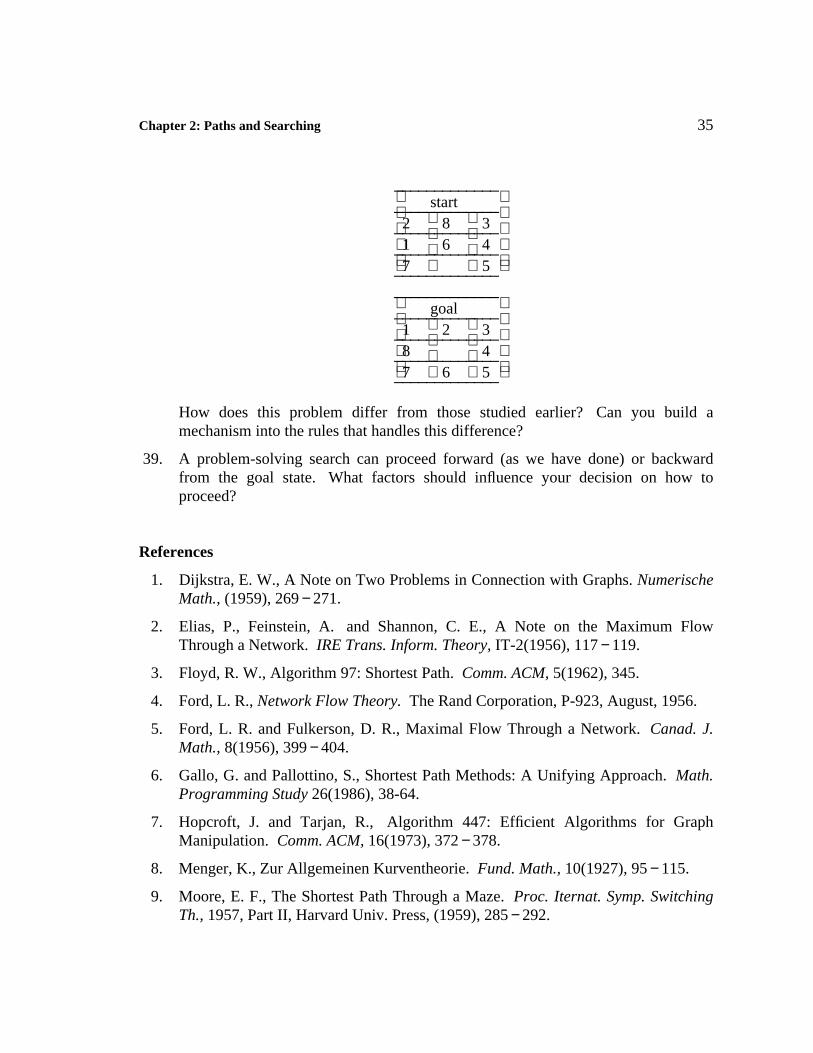
38. The 8-puzzle is a square tray in which are placed eight numbered tiles. Theremaining ninth square is open. A tile that is adjacent to the open square can slideinto that space. The object of this game is to obtain the following configurationfrom the starting configuration:


_____________start_____________

2 8 3_____________1 6 4_____________7 5_____________

_____________goal_____________

1 2 3_____________8 4_____________7 6 5_____________

How does this problem differ from those studied earlier? Can you build amechanism into the rules that handles this difference?

39. A problem-solving search can proceed forward (as we have done) or backwardfrom the goal state. What factors should influence your decision on how toproceed?

References

1. Dijkstra, E. W., A Note on Two Problems in Connection with Graphs. NumerischeMath., (1959), 269 − 271.

2. Elias, P., Feinstein, A. and Shannon, C. E., A Note on the Maximum FlowThrough a Network. IRE Trans. Inform. Theory, IT-2(1956), 117 − 119.

3. Floyd, R. W., Algorithm 97: Shortest Path. Comm. ACM, 5(1962), 345.

4. Ford, L. R., Network Flow Theory. The Rand Corporation, P-923, August, 1956.

5. Ford, L. R. and Fulkerson, D. R., Maximal Flow Through a Network. Canad. J.Math., 8(1956), 399 − 404.

6. Gallo, G. and Pallottino, S., Shortest Path Methods: A Unifying Approach. Math.Programming Study 26(1986), 38-64.

7. Hopcroft, J. and Tarjan, R., Algorithm 447: Efficient Algorithms for GraphManipulation. Comm. ACM, 16(1973), 372 − 378.

8. Menger, K., Zur Allgemeinen Kurventheorie. Fund. Math., 10(1927), 95 − 115.

9. Moore, E. F., The Shortest Path Through a Maze. Proc. Iternat. Symp. SwitchingTh., 1957, Part II, Harvard Univ. Press, (1959), 285 − 292.


10. Tarjan, R., Depth-First Search and Linear Graph Algorithms. SIAM J. Comput.,1(1972), 146 − 160.

11. Tremaux: see Lucas, E., Recreations Mathematiques. Paris, 1982.

12. Whitney, H., Congruent Graphs and the Connectivity of Graphs. Amer. J. Math.,54(1932), 150 − 168.

Documents

Chapter 2 Paths and Searching - Department of …rg/book/chap2.pdf2 Chapter 2: Paths and Searching graph. We now have a very general and ﬂexible idea of distance that applies in