Chapter 2 Numeric, Cell, and Structure Arraysmzali/courses/Fall14/Arch 754/slides/Chapter 3.pdf · ... denotes all the elements in the second through fifth columns ... v consisting

Chapter 2

Numeric, Cell, and Structure Arrays

Vectors: To create a row vector, separate the

elements by semicolons. Use square brackets.

For example,

>>p = [3,7,9]

p =

3 7 9

You can create a column vector by using the

transpose notation (').

>>p = [3,7,9]'

p =

3

7

9

2-2

You can also create a column vector by separating the

elements by semicolons. For example,

>>g = [3;7;9]

g =

3

7

9

2-3

2-4

You can create vectors by ''appending'' one vector to

another.

For example, to create the row vector u whose first three

columns contain the values of r = [2,4,20] and

whose fourth, fifth, and sixth columns contain the values of w = [9,-6,3], you type u = [r,w]. The result is

the vector u = [2,4,20,9,-6,3].

The colon operator (:) easily generates a large vector of

regularly spaced elements. Parentheses are not needed

but can be used for clarity. Do not use square brackets.

Typing

>>x = m:q:n

or

>>x = (m:q:n)

creates a vector x of values with a spacing q. The first

value is m. The last value is n if m - n is an integer

multiple of q. If not, the last value is less than n.

2-5

For example, typing x = 0:2:8 creates the

vector x = [0,2,4,6,8], whereas typing x =

0:2:7 creates the vector x = [0,2,4,6].

To create a row vector z consisting of the values from 5 to 8 in steps of 0.1, type z = 5:0.1:8.

If the increment q is omitted, it is presumed to be 1. Thus typing y = -3:2 produces the vector y

= [-3,-2,-1,0,1,2].

2-6

The linspace command also creates a linearly

spaced row vector, but instead you specify the number

of values rather than the increment.

The syntax is linspace(x1,x2,n), where x1 and x2

are the lower and upper limits and n is the number of

points.

For example, linspace(5,8,31) is equivalent to

5:0.1:8.

If n is omitted, the spacing is 1.

2-7

The logspace command creates an array of

logarithmically spaced elements.

Its syntax is logspace(a,b,n), where n is

the number of points between 10a and 10b.

For example, x = logspace(-1,1,4)

produces the vector x = [0.1000,

0.4642, 2.1544, 10.000].

If n is omitted, the number of points defaults to

50.

2-8

More? See page 56.

Magnitude, Length, and Absolute Value of a Vector

Keep in mind the precise meaning of these terms when

using MATLAB.

The length command gives the number of elements in

the vector.

The magnitude of a vector x having elements x1, x2, …,

xn is a scalar, given by x12 + x2

2 + … + xn2), and is the

same as the vector's geometric length.

The absolute value of a vector x is a vector whose

elements are the absolute values of the elements of x.

2-9

For example, if x = [2,-4,5],

its length is 3; (computed from length(x))

its magnitude is [22 + (–4)2 + 52] = 6.7082;

(computed from sqrt(x’*x))

its absolute value is [2,4,5] (computed

from abs(x)).

2-10

More? See pages 61-62.

Matrices

A matrix has multiple rows and columns. For

example, the matrix

has four rows and three columns.

Vectors are special cases of matrices having

one row or one column.

M =2 4 10

16 3 7

8 4 9

3 12 15

2-11


Creating Matrices

If the matrix is small you can type it row by row, separating

the elements in a given row with spaces or commas and

separating the rows with semicolons. For example, typing

>>A = [2,4,10;16,3,7];

creates the following matrix:

2 4 10

16 3 7

Remember, spaces or commas separate elements in

different columns, whereas semicolons separate elements

in different rows.

A =

2-12

Creating Matrices from Vectors

Suppose a = [1,3,5] and b = [7,9,11] (row

vectors). Note the difference between the results given by [a b] and [a;b] in the following session:

>>c = [a b];

c =

1 3 5 7 9 11

>>D = [a;b]

D =

1 3 5

7 9 11

2-13

You need not use symbols to create a new array.

For example, you can type

>> D = [[1,3,5];[7,9,11]];

2-14

Array Addressing

The colon operator selects individual elements, rows,columns, or ''subarrays'' of arrays. Here are some examples:

■ v(:) represents all the row or column elements of the vector v.

■ v(2:5) represents the second through fifth elements; that is v(2), v(3), v(4), v(5).

Array Addressing, continued

A(:,3) denotes all the elements in the third column of the matrix A.

A(:,2:5) denotes all the elements in the second through fifth columns of A.

A(2:3,1:3) denotes all the elements in the second and third rows that are also in the first through third columns.

v = A(:) creates a vector v consisting of all the

columns of A stacked from first to last.

A(end,:) denotes the last row in A, and A(:,end)

denotes the last column.

2-15

You can use array indices to extract a smaller array from

another array. For example, if you first create the array B

B =

2-16

C =16 3 7

8 4 9

2 4 10 13

16 3 7 18

8 4 9 25

3 12 15 17

then type C = B(2:3,1:3), you can produce the

following array:


Additional Array Functions (Table 2.1–1 on page 60)

[u,v,w] =

find(A)

length(A)

Computes the arrays u and v, containing the row and column indices of the nonzero elements of the matrix A, and the array w, containing the values of the nonzero elements. The array w

may be omitted.

Computes either the number of elements of A if A is a vector or the largest value of m or n if A is an m × n matrix.

2-17

Additional Array Functions (Table 2.1–1)

max(A) Returns the algebraically largest element in A if A

is a vector.

Returns a row vector

containing the largest

elements in each column if A is a matrix.

If any of the elements are complex, max(A) returns

the elements that have

the largest magnitudes.

2-18


[x,k] =

max(A)

min(A)

and

[x,k] =

min(A)

Similar to max(A) but stores the maximum values in the row vector xand their indices in the row vector k.

Like max but returns minimum values.

2-19

2-20

size(A) Returns a row vector [m n]

containing the sizes of them x n array A.

sort(A) Sorts each column of the

array A in ascending order

and returns an array the same size as A.

sum(A) Sums the elements in each

column of the array A and

returns a row vector

containing the sums.


The function size(A) returns a row vector [m n]

containing the sizes of the m × n array A. The length(A) function computes either the number of

elements of A if A is a vector or the largest value of m or

n if A is an m × n matrix.

For example, if

then max(A) returns the vector [6,2]; min(A)returns

the vector [-10, -5]; size(A) returns [3, 2]; and

length(A) returns 3.

A =

6 2

–10 –5

3 0

2-21 More? See pages 59-61.

The Workspace Browser. Figure 2.1–1

2-22

See page 62

The Variable Editor. Figure 2.1–2

2-23

See page 63

Multidimensional Arrays

Consist of two-dimensional matrices “layered” to produce a

third dimension. Each “layer” is called a page.

cat(n,A,B,C, ...) Creates a new array by

concatenating the arrays A,B,C, and so

on along the dimension n.

2-24


Array Addition and Subtraction

6 –2

10 3+

9 8

–12 14=

15 6

–2 17

Array subtraction is performed in a similar way.

The addition shown in equation 2.3–1 is performed in

MATLAB as follows:

>>A = [6,-2;10,3];

>>B = [9,8;-12,14]

>>A+B

ans =

15 6

-2 17

For example:

2-25

(2.3-1)

More? See page 65.

Multiplication: Multiplying a matrix A by a scalar w

produces a matrix whose elements are the elements of

A multiplied by w. For example:

32 9

5 –7=

6 27

15 –21

This multiplication is performed in MATLAB as follows:

>>A = [2, 9; 5,-7];

>>3*A

ans =

6 27

15 -21

2-26

Multiplication of an array by a scalar is easily defined

and easily carried out.

However, multiplication of two arrays is not so

straightforward.

MATLAB uses two definitions of multiplication:

(1) array multiplication (also called element-by-element

multiplication), and

(2) matrix multiplication.

2-27

Division and exponentiation must also be

carefully defined when you are dealing

with operations between two arrays.

MATLAB has two forms of arithmetic

operations on arrays. Next we introduce

one form, called array operations, which

are also called element-by-element

operations. Then we will introduce matrix

operations. Each form has its own

applications.

Division and exponentiation must also be

carefully defined when you are dealing

with operations between two arrays.

2-28

Element-by-element operations: Table 2.3–1 on page 66

Symbol

+

-

+

-

.*

./

.\

.^

Examples

[6,3]+2=[8,5]

[8,3]-5=[3,-2]

[6,5]+[4,8]=[10,13]

[6,5]-[4,8]=[2,-3]

[3,5].*[4,8]=[12,40]

[2,5]./[4,8]=[2/4,5/8]

[2,5].\[4,8]=[2\4,5\8]

[3,5].^2=[3^2,5^2]

2.^[3,5]=[2^3,2^5]

[3,5].^[2,4]=[3^2,5^4]

Operation

Scalar-array addition

Scalar-array subtraction

Array addition

Array subtraction

Array multiplication

Array right division

Array left division

Array exponentiation

Form

A + b

A – b

A + B

A – B

A.*B

A./B

A.\B

A.^B

2-29

Array or Element-by-element multiplication is defined only

for arrays having the same size. The definition of the product x.*y, where x and y each have n elements, is

x.*y = [x(1)y(1), x(2)y(2), ... , x(n)y(n)]

if x and y are row vectors. For example, if

x = [2, 4, – 5], y = [– 7, 3, – 8] (2.3–4)

then z = x.*y gives

z = [2(– 7), 4 (3), –5(–8)] = [–14, 12, 40]

2-30

If x and y are column vectors, the result of x.*y is a

column vector. For example z = (x’).*(y’) gives

Note that x’ is a column vector with size 3 × 1 and thus

does not have the same size as y, whose size is 1 × 3.

Thus for the vectors x and y the operations x’.*y and

y.*x’ are not defined in MATLAB and will generate an

error message.

2(–7)

4(3)

–5(–8)

–14

12

40=z =

2-31

The array operations are performed between the

elements in corresponding locations in the arrays. For example, the array multiplication operation A.*B results

in a matrix C that has the same size as A and B and has

the elements ci j = ai j bi j . For example, if

then C = A.*B gives this result:

A = 11 5

–9 4B =

–7 8

6 2

C = 11(–7) 5(8)

–9(6) 4(2)=

–77 40

–54 8

2-32

More? See page 66.

The built-in MATLAB functions such as sqrt(x) and

exp(x) automatically operate on array arguments to

produce an array result the same size as the array argument x.

Thus these functions are said to be vectorized functions.

For example, in the following session the result y has

the same size as the argument x.

>>x = [4, 16, 25];

>>y = sqrt(x)

y =

2 4 5

2-33

However, when multiplying or dividing these

functions, or when raising them to a power,

you must use element-by-element operations if

the arguments are arrays.

For example, to compute z = (ey sin x) cos2x,

you must type

z = exp(y).*sin(x).*(cos(x)).^2.

You will get an error message if the size of x is

not the same as the size of y. The result z will

have the same size as x and y.


Array Division

The definition of array division is similar to the definition

of array multiplication except that the elements of one

array are divided by the elements of the other array.

Both arrays must have the same size. The symbol for

array right division is ./. For example, if

x = [8, 12, 15] y = [–2, 6, 5]

then z = x./y gives

z = [8/(–2), 12/6, 15/5] = [–4, 2, 3]

2-35

A = 24 20

– 9 4B =

–4 5

3 2

Also, if

then C = A./B gives

C = 24/(–4) 20/5

–9/3 4/2=

–6 4

–3 2

2-36


Array Exponentiation

MATLAB enables us not only to raise arrays to powers

but also to raise scalars and arrays to array powers.

To perform exponentiation on an element-by-element basis, we must use the .^ symbol.

For example, if x = [3, 5, 8], then typing x.^3

produces the array [33, 53, 83] = [27, 125, 512].

2-37

We can raise a scalar to an array power. For example, if p = [2, 4, 5], then typing 3.^p produces the array

[32, 34, 35] = [9, 81, 243].

Remember that .^ is a single symbol. The dot in 3.^p

is not a decimal point associated with the number 3. The following operations, with the value of p given here, are

equivalent and give the correct answer:

3.^p

3.0.^p

3..^p

(3).^p

3.^[2,4,5]


Matrix-Matrix Multiplication

In the product of two matrices AB, the number of

columns in A must equal the number of rows in B. The

row-column multiplications form column vectors, and

these column vectors form the matrix result. The

product AB has the same number of rows as A and the

same number of columns as B. For example,

6 –2

10 3

4 7

9 8

–5 12=

(6)(9) + (– 2)(– 5) (6)(8) + (– 2)(12)

(10)(9) + (3)(– 5) (10)(8) + (3)(12)

(4)(9) + (7)(– 5) (4)(8) + (7)(12)

64 24

75 116

1 116

= (2.4–4)

2-39

Use the operator * to perform matrix multiplication in

MATLAB. The following MATLAB session shows how to

perform the matrix multiplication shown in (2.4–4).

>>A = [6,-2;10,3;4,7];

>>B = [9,8;-5,12];

>>A*B

ans =

64 24

75 116

1 116

2-40

Matrix multiplication does not have the commutative

property; that is, in general, AB BA. A simple

example will demonstrate this fact:

AB = 6 –2

10 3

9 8

–12 14=

78 20

54 122

BA = 9 8

–12 14

6 –2

10 3=

134 6

68 66

whereas

Reversing the order of matrix multiplication is a

common and easily made mistake.

2-41


Special Matrices (Pages 82-83)

Two exceptions to the noncommutative property are the

null or zero matrix, denoted by 0 and the identity, or

unity, matrix, denoted by I.

The null matrix contains all zeros and is not the same

as the empty matrix [ ], which has no elements.

These matrices have the following properties:

0A = A0 = 0

IA = AI = A

2-42

The identity matrix is a square matrix whose diagonal

elements are all equal to one, with the remaining

elements equal to zero.

For example, the 2 × 2 identity matrix is

I = 1 0

0 1

The functions eye(n) and eye(size(A)) create an

n × n identity matrix and an identity matrix the same size as the matrix A.

2-43

Sometimes we want to initialize a matrix to have all zero elements. The zeros command creates a matrix of all

zeros.

Typing zeros(n) creates an n × n matrix of zeros,

whereas typing zeros(m,n) creates an m × n matrix of

zeros.

Typing zeros(size(A)) creates a matrix of all zeros

having the same dimension as the matrix A. This type of

matrix can be useful for applications in which we do not

know the required dimension ahead of time.

The syntax of the ones command is the same, except

that it creates arrays filled with ones.

2-44More? See page 83.

Matrix Left Division and Linear Algebraic

Equations (Page 84)

6x + 12y + 4z = 70

7x – 2y + 3z = 5

2x + 8y – 9z = 64

>>A = [6,12,4;7,-2,3;2,8,-9];

>>B = [70;5;64];

>>Solution = A\B

Solution =

3

5

-2

The solution is x = 3, y = 5, and z = –2.

2-45

Polynomial Coefficients

The function poly(r)computes the coefficients of the

polynomial whose roots are specified by the vector r.

The result is a row vector that contains the polynomial’s

coefficients arranged in descending order of power.

For example,

>>c = poly([-2, -5])

c =

1 7 10

2-46

More? See page 95.

Polynomial Roots

The function roots(a)computes the roots of a polynomial

specified by the coefficient array a. The result is a

column vector that contains the polynomial’s roots.

For example,

>>r = roots([2, 14, 20])

r =

-2

-5

2-47

More? See page 95.

Polynomial Multiplication and Division

The function conv(a,b) computes the product of the two

polynomials described by the coefficient arrays a and b.

The two polynomials need not be the same degree. The

result is the coefficient array of the product polynomial.

The function [q,r] = deconv(num,den) computes the

result of dividing a numerator polynomial, whose coefficient array is num, by a denominator polynomial

represented by the coefficient array den. The quotient

polynomial is given by the coefficient array q, and the

remainder polynomial is given by the coefficient array r.

2-48

Polynomial Multiplication and Division: Examples

>>a = [9,-5,3,7];

>>b = [6,-1,2];

>>product = conv(a,b)

product =

54 -39 41 29 -1 14

>>[quotient, remainder] = deconv(a,b)

quotient =

1.5 -0.5833

remainder =

0 0 -0.5833 8.1667

2-49


Plotting Polynomials

The function polyval(a,x)evaluates a polynomial at

specified values of its independent variable x, which can

be a matrix or a vector. The polynomial’s coefficients of descending powers are stored in the array a. The result

is the same size as x.

2-50

Example of Plotting a Polynomial

To plot the polynomial f (x) = 9x3 – 5x2 + 3x + 7

for -2 ≤ x ≤ 5, you type

>>a = [9,-5,3,7];

>>x = -2:0.01:5;

>>f = polyval(a,x);

>>plot(x,f),xlabel(’x’),ylabel(’f(x)’)

2-51

More? See page 97.

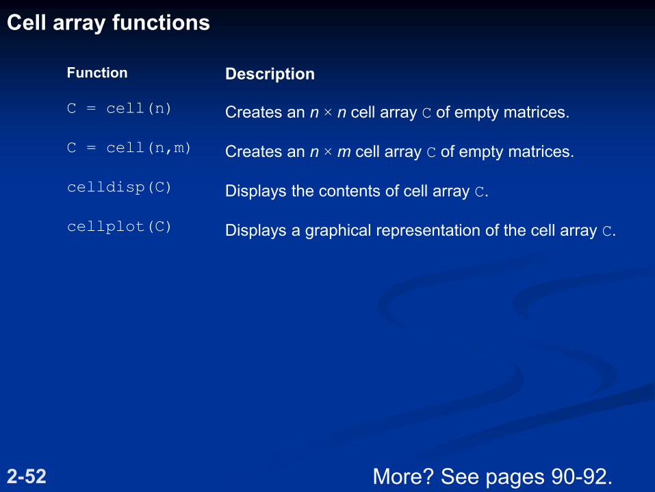
Function

C = cell(n)

C = cell(n,m)

celldisp(C)

cellplot(C)

Description

Creates an n × n cell array C of empty matrices.

Creates an n × m cell array C of empty matrices.

Displays the contents of cell array C.

Displays a graphical representation of the cell array C.

Cell array functions


Arrangement of data in the structure array student.

Figure 2.7–1 on page 92.

2-53

Function

names = fieldnames(S)

isfield(S,’field’)

isstruct(S)

Description

Returns the field names

associated with the

structure array S as names,

a cell array of strings.

Returns 1 if ’field’ is the

name of a field in the

structure array S, and 0

otherwise.

Returns 1 if the array S is a

structure and 0 otherwise.

Structure functions Table 2.7–1 on page 94

2-54

Structure functions Table 2.7–1 (continued)

S =

rmfield(S,’field’)

S = struct(’f1’,’v1’,

’f2’,’v2’,...)

Removes the field ’field’

from the structure array S.

Creates a structure array with the fields ’f1’, ’f2’, .

. . having the values ’v1’,

’v2’, . . . .

2-55

More? See pages 92-96

Documents

Chapter 2 Numeric, Cell, and Structure Arraysmzali/courses/Fall14/Arch 754/slides/Chapter 3.pdf · ... denotes all the elements in the second through fifth columns ... v consisting