Embed Size (px)
Citation preview
The Practice of Statistics, 5th Edition
Starnes, Tabor, Yates, Moore
Bedford Freeman Worth Publishers
CHAPTER 2 Modeling Distributions of Data 2.2 Density Curves and
Normal Distributions
Learning Objectives
After this section, you should be able to:
The Practice of Statistics, 5th Edition 2
Density Curves: define and describe the mean and median location
Normal Distribution: estimate areas/ proportion of values/
probability. Use 68-95-99.7 Rule
The Standard normal distribution: find the proportion of z-values in
a specified interval, or a z-score from a percentile in the standard
Normal distribution.
Density Curves and Normal Distributions
The Practice of Statistics, 5th Edition 3
Exploring Quantitative Data
1. Always plot your data: make a graph, usually a dotplot, stemplot, or histogram.
2. Look for the overall pattern (shape, center, and spread) and for striking departures such as outliers.
3. Calculate a numerical summary to briefly describe center and spread.
Exploring Quantitative Data
4. Sometimes the overall pattern of a large number of
observations is so regular that we can describe it by a
smooth curve.
The Practice of Statistics, 5th Edition 4
Density Curves
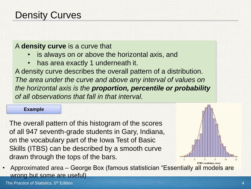
A density curve is a curve that
• is always on or above the horizontal axis, and
• has area exactly 1 underneath it.
A density curve describes the overall pattern of a distribution.
The area under the curve and above any interval of values on
the horizontal axis is the proportion, percentile or probability
of all observations that fall in that interval.
The overall pattern of this histogram of the scores
of all 947 seventh-grade students in Gary, Indiana,
on the vocabulary part of the Iowa Test of Basic
Skills (ITBS) can be described by a smooth curve
drawn through the tops of the bars.
Example
• Approximated area – George Box (famous statistician “Essentially all models are
wrong but some are useful)
The Practice of Statistics, 5th Edition 5
Batting averages
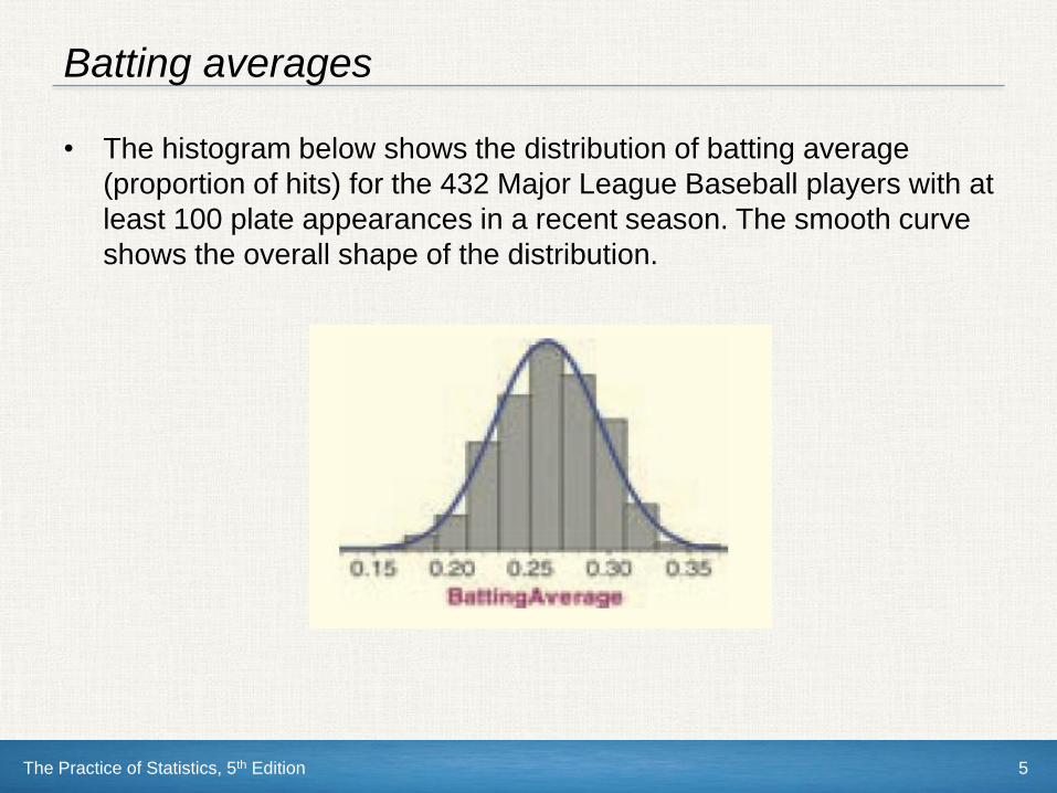
• The histogram below shows the distribution of batting average
(proportion of hits) for the 432 Major League Baseball players with at
least 100 plate appearances in a recent season. The smooth curve
shows the overall shape of the distribution.
The Practice of Statistics, 5th Edition 6
Describing Density Curves: measure of center
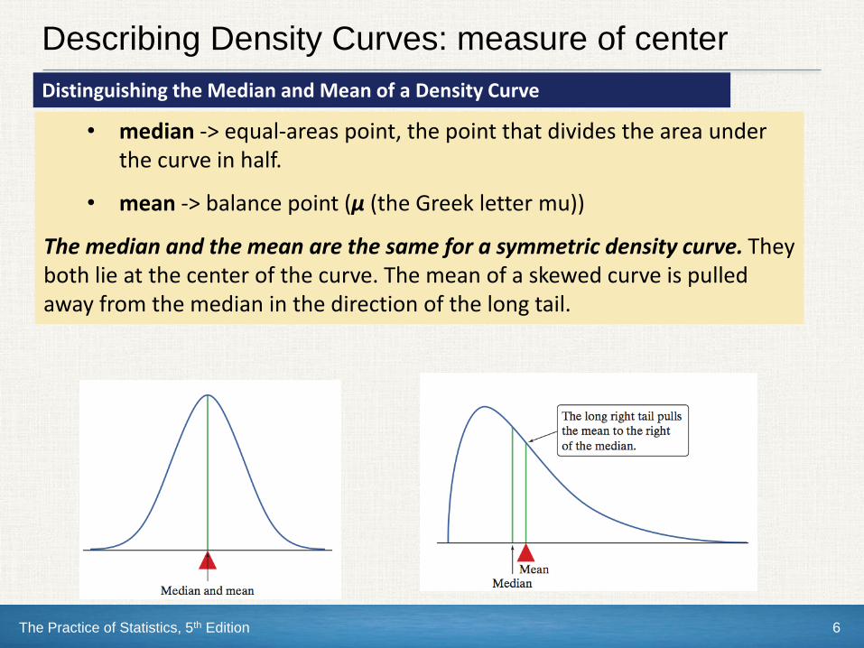
• median -> equal-areas point, the point that divides the area under the curve in half.
• mean -> balance point (µ (the Greek letter mu))
The median and the mean are the same for a symmetric density curve. They both lie at the center of the curve. The mean of a skewed curve is pulled away from the median in the direction of the long tail.
Distinguishing the Median and Mean of a Density Curve
The Practice of Statistics, 5th Edition 7
The Practice of Statistics, 5th Edition 8
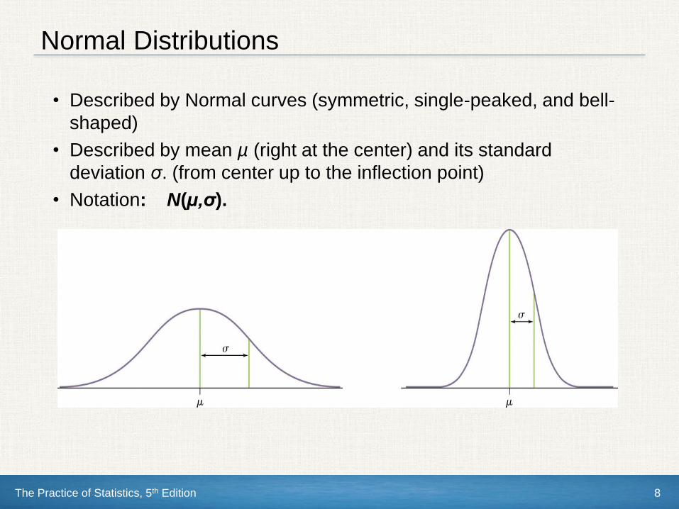
Normal Distributions
• Described by Normal curves (symmetric, single-peaked, and bell-
shaped)
• Described by mean µ (right at the center) and its standard
deviation σ. (from center up to the inflection point)
• Notation: N(µ,σ).
The Practice of Statistics, 5th Edition 9
Why are Normal Distributions important?
• Normal distributions are good descriptions for some distributions of real
data.(scores on tests, repeated measurements on volleyball diameter.
Characteristics of biological population)
• Normal distributions are good approximations of the results of many
kinds of chance outcomes (number of heads in many tosses with fair
coin).
• Many statistical inference procedures are based on Normal distributions.
The Practice of Statistics, 5th Edition 10
Discovery Applet Activity
• Follow instructions on page 110
• http://bcs.whfreeman.com/tps5e/default.asp#923932__929331__
• Summarize: For any normal density curve, the area under the curve
within one, two or three standard deviations of the mean is about
____% ____% ____%.
• Page: 110 read, + example page 11
The Practice of Statistics, 5th Edition 11
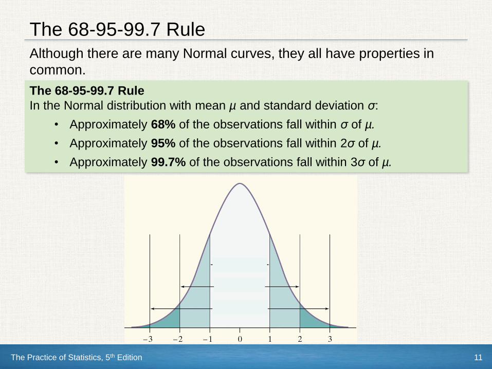
The 68-95-99.7 Rule Although there are many Normal curves, they all have properties in
common.
The 68-95-99.7 Rule
In the Normal distribution with mean µ and standard deviation σ:
• Approximately 68% of the observations fall within σ of µ.
• Approximately 95% of the observations fall within 2σ of µ.
• Approximately 99.7% of the observations fall within 3σ of µ.
The Practice of Statistics, 5th Edition 12
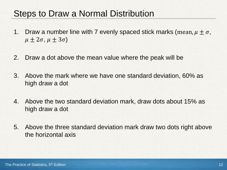
Steps to Draw a Normal Distribution
1. Draw a number line with 7 evenly spaced stick marks (mean, 𝜇 ± 𝜎,
𝜇 ± 2𝜎, 𝜇 ± 3𝜎)
2. Draw a dot above the mean value where the peak will be
3. Above the mark where we have one standard deviation, 60% as
high draw a dot
4. Above the two standard deviation mark, draw dots about 15% as
high draw a dot
5. Above the three standard deviation mark draw two dots right above
the horizontal axis
The Practice of Statistics, 5th Edition 13
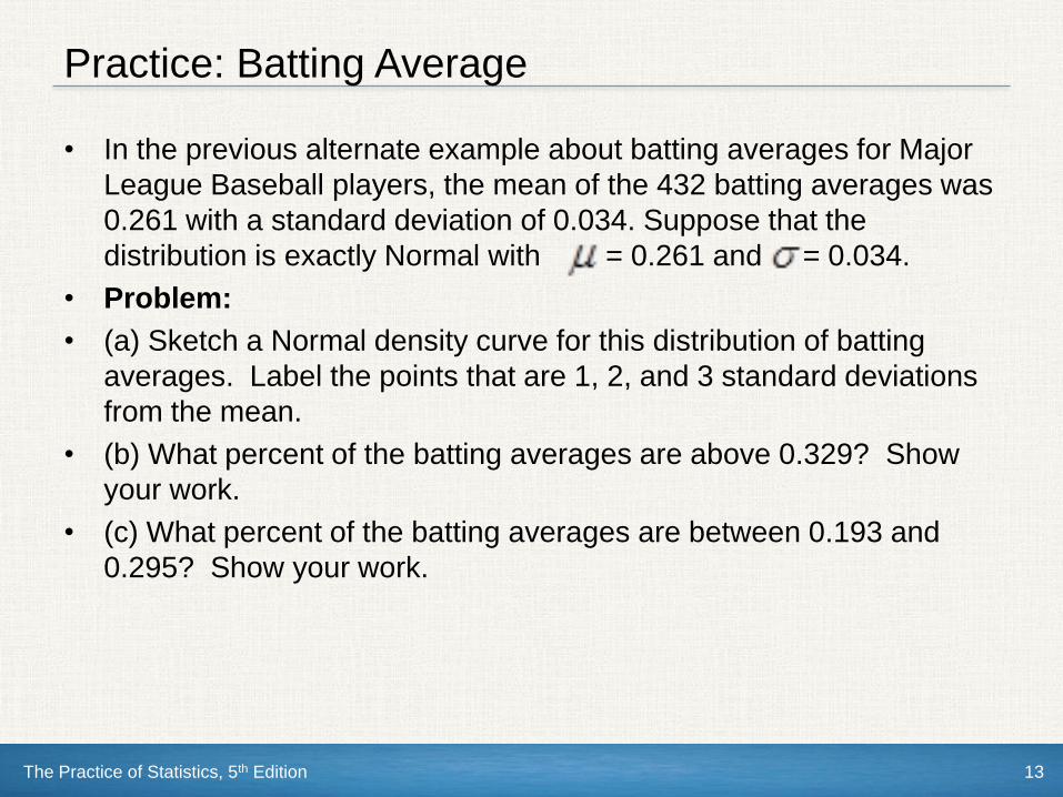
Practice: Batting Average
• In the previous alternate example about batting averages for Major
League Baseball players, the mean of the 432 batting averages was
0.261 with a standard deviation of 0.034. Suppose that the
distribution is exactly Normal with = 0.261 and = 0.034.
• Problem:
• (a) Sketch a Normal density curve for this distribution of batting
averages. Label the points that are 1, 2, and 3 standard deviations
from the mean.
• (b) What percent of the batting averages are above 0.329? Show
your work.
• (c) What percent of the batting averages are between 0.193 and
0.295? Show your work.
The Practice of Statistics, 5th Edition 14
The Practice of Statistics, 5th Edition 15
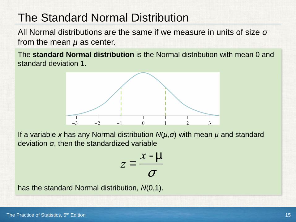
The Standard Normal Distribution All Normal distributions are the same if we measure in units of size σ
from the mean µ as center.
The standard Normal distribution is the Normal distribution with mean 0 and
standard deviation 1.
If a variable x has any Normal distribution N(µ,σ) with mean µ and standard
deviation σ, then the standardized variable
has the standard Normal distribution, N(0,1).
z =x - m
s
The Practice of Statistics, 5th Edition 16
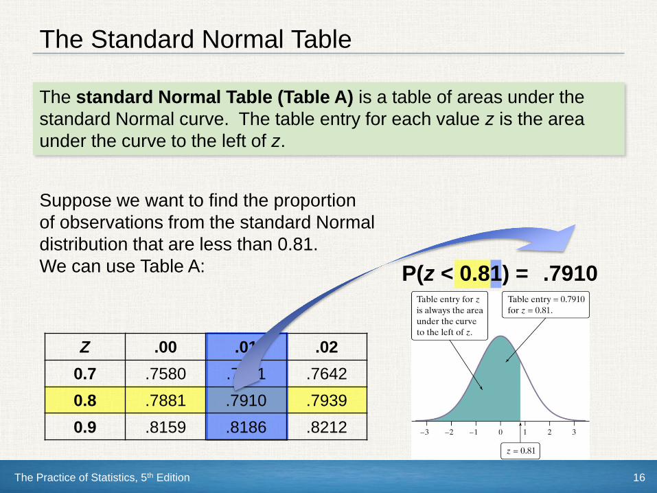
The Standard Normal Table
The standard Normal Table (Table A) is a table of areas under the
standard Normal curve. The table entry for each value z is the area
under the curve to the left of z.
Z .00 .01 .02
0.7 .7580 .7611 .7642
0.8 .7881 .7910 .7939
0.9 .8159 .8186 .8212
P(z < 0.81) = .7910
Suppose we want to find the proportion
of observations from the standard Normal
distribution that are less than 0.81.
We can use Table A:
The Practice of Statistics, 5th Edition 17
The Practice of Statistics, 5th Edition 18
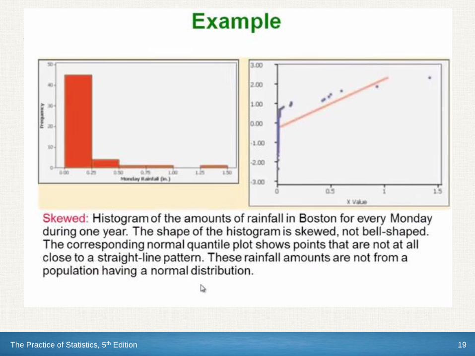
The Practice of Statistics, 5th Edition 19
The Practice of Statistics, 5th Edition 20
Page 114 problem
• Practice (you’ll be asked to find L , R tail area and in between z-
scores)
Finding areas under the standard Normal curve
Problem: Find the proportion of observations from the standard Normal
distribution that are between −0.58 and 1.79.
The Practice of Statistics, 5th Edition 21
Homework
• Calculator Activity (in the AP exam choose whichever method is
easiest: table A or calculator)
• Page 128 # 33 to 51