Embed Size (px)
Citation preview

Chapter 2
Measure spaces
2.1 Sets and �-algebras
2.1.1 Definitions
Let X be a (non-empty) set; at this stage it is only a set, i.e., not yet endowed withany additional structure. Our eventual goal is to define a measure on subsets ofX. As we have seen, we may have to restrict the subsets to which a measure isassigned. There are, however, certain requirements that the collection of sets towhich a measure is assigned—measurable sets (�;&$*$/ ;&7&"8)—should satisfy.If two sets are measurable, we would like their union, intersection and comple-ments to be measurable as well. This leads to the following definition:
Definition 2.1 LetX be a non-empty set. A (boolean) algebra of subsets (%9"#-!�;&7&"8 -:) of X, is a non-empty collection of subsets of X, closed under finiteunions (�*5&2 $&(*!) and complementation. A (boolean) �-algebra (�%9"#-! %/#*2)⌃ of subsets ofX is a non-empty collection of subsets ofX, closed under countableunions (�%**1/ 0" $&(*!) and complementation.
Comment: In the context of probability theory, the elements of a �-algebra arecalled events (�;&39&!/).
Proposition 2.2 Let A be an algebra of subsets of X. Then, A contains X, theempty set, and it is closed under finite intersections.
8 Chapter 2
Proof : Since A is not empty, it contains at least one set A ∈ A. Then,
X = A ∪ Ac ∈ A and � = Xc ∈ A.Let A1, . . . ,An ⊂ A. By de Morgan’s laws,
n�k=1
Ak = � n�k=1
Ack�
c ∈ A.n
Given in 2018
. Exercise 2.1 Let X be a set and let A be a collection of subsets containing X and closedunder set subtraction (i.e, if A,B ∈ A then A � B ∈ A. Show that A is an algebra.
The following useful proposition states that for an algebra to be a �-algebra, itsu�ces to require closure under countable disjoint union:
Proposition 2.3 Let X be a non-empty set, and let A ⊂ P(X) be an algebra ofsubsets of X, closed under countable disjoint unions. Then, A is a �-algebra.
Proof : We need to show that A is closed under countable unions. Let (An) ⊂ A,and define recursively the sequence of disjoint sets (Bn),
B1 = A1 ∈ A and Bn = An � �n−1�k=1
Ak� ∈ A.Then, ∞�
n=1An = ∞�
n=1Bn ∈ A.
(The inclusion �∞n=1 Bn ⊂ �∞n=1 An is obvious. Let x ∈ �∞n=1 An. Then, there exists aminimal n such that x ∈ An. By definition of the Bn’s, x ∈ Bn, hence x ∈ �∞n=1 Bn,which proves the reverse inclusion.) n
Trick #1: Turn a sequence of sets into a sequence of disjoint sets having the sameunion.—1h(2018)—
Definition 2.4 A non-empty set endowed with a �-algebra of subsets is called ameasurable space (�$*$/ "(9/).

Measure spaces 9
To conclude, a �-algebra is a collection of sets closed under countably-many set-theoretic operations.
Examples:
1. Let X be a non-empty set. Then,
{�,X}is its smallest �-algebra (the trivial �-algebra).
2. Let X be a non-empty set. Then, its power set (�%8'(% ;7&"8) P(X) is itsmaximal �-algebra.
3. Let X be a non-empty set. Then,
⌃ = {A ⊂ X ∶ A is countable or Ac is countable}is a �-algebra (the countable or co-countable sets). Clearly, ⌃ is non-empty and is closed under complementation. Let (An) ⊂ ⌃. If all An arecountable, then their union is also countable, hence in ⌃. Conversely, if oneof the An is co-countable, then their union is also co-countable, hence in ⌃.
The following proposition states that every intersection of �-algebras is a �-algebra. This property will be used right after to prove that every collection ofsubsets defines a unique �-algebra, which is the smallest �-algebra containingthat collection.
Proposition 2.5 Let {⌃↵ ⊂ P(X) ∶ ↵ ∈ J} be a (not necessarily countable)collection of �-algebras. Then, their intersection is a �-algebra.
Proof : Set⌃ = �
↵∈J ⌃↵.
Since for every ↵ ∈ J, �,X ∈ ⌃↵, it follows that ⌃ contains � and X. Let A ∈ ⌃; bydefinition,
A ∈ ⌃↵ ∀↵ ∈ J.

10 Chapter 2
Since each of the ⌃↵ is a �-algebra,
Ac ∈ ⌃↵ ∀↵ ∈ J,
hence Ac ∈ ⌃, proving that ⌃ is closed under complementation. Likewise, let(An) ⊂ ⌃. Then,An ∈ ⌃↵ ∀n ∈ N and ∀↵ ∈ J.
It follows that ∞�n=1
An ∈ ⌃↵ ∀↵ ∈ J,
hence ∞�n=1
An ∈ ⌃,proving that ⌃ is closed under countable unions. n
. Exercise 2.2 Let X be a set. (a) Show that the collection of subsets that are either finite orco-finite is an algebra. (b) Show that it is a �-algebra if and only if X is a finite set.
Given in 2018
. Exercise 2.3 (a) Let An be an increasing sequence of algebras of subsets of X, i.e., An ⊂An+1. Show that
A = ∞�n=1An
is an algebra. (b) Give an example in which An is an increasing sequence of �-algebras, and itsunion is not a �-algebra.
Let E ⊂P(X) be a collection of sets and consider the family of all �-algebras ofsubsets of X containing E . This family is not empty since is includes at least thepower set P(X). By Proposition 2.5,
�(E) =�{⌃ ∶ ⌃ is a �-algebra containing E}is a �-algebra; it is the smallest �-algebra containing E ; it is called the �-algebragenerated by (�*$* -3 ;97&1) E .A comment about nomenclature: we will repeatedly deal with sets of sets and setsof sets of sets; to avoid confusion, we will use the terms collection (�42&!), class(�%8-(/) and family (�%(5:/) for sets whose elements are sets.The following proposition comes up useful:

Measure spaces 11
Proposition 2.6 Let E ⊂P(X) and let ⌃ ⊂P(X) be a �-algebra. If
E ⊂ ⌃,then
�(E) ⊂ ⌃.
Proof : Since ⌃ is a �-algebra containing E , then, by definition, it contains �(E).n
Corollary 2.7 Let E ,F ⊂P(X). If
E ⊂ �(F) and F ⊂ �(E),then
�(E) = �(F).
. Exercise 2.4 Let X be a non-countable set. Let
E = {{x} ∶ x ∈ X}.What is the �-algebra generated by E?
. Exercise 2.5 Let A1, . . . ,An be a finite number of subsets of X.
(a) Prove that if the A1, . . . ,An are disjoint and their union is X, then
��({A1, . . . ,An})� = 2n.
(b) Prove that for arbitrary A1, . . . ,An,
�({A1, . . . ,An})contains a finite number of elements.
. Exercise 2.6 Let (X,⌃) be a measurable space. Let C be a collection of sets. Let P be aproperty of sets in X (i.e., a function P ∶P(X)→ {true, false}), such that
(a) P(�) = true.

12 Chapter 2
(b) P(C) = true for all C ∈ C.
(c) P(A) = true implies that P(Ac) = true.
(d) if P(An) = true for all n, then P(�∞n=1 An) = true.
Show that P(A) = true for all A ∈ �(C).Given in 2018
. Exercise 2.7 Prove that every member of a �-algebra is countably-generated: i.e., let Cbe a collection of subsets of X and let A ∈ �(C). Prove that there exists a countable sub-collectionCA ⊂ C, such that A ∈ �(CA).
Given in 2018
. Exercise 2.8 Let f ∶ X1 → X2 be a function between two sets. Prove that if ⌃2 is a �-algebra on X2, then
⌃1 = { f −1(A) ∶ A ∈ ⌃2}is a �-algebra on X1.
Given in 2018
. Exercise 2.9 Let (X,⌃) be a measurable space and let An ∈ ⌃ be a sequence of measurableset. The superior limit of this sequence is the set of points x which belong to An for infinitely-many n’s, i.e.,
lim supn→∞ An = {x ∈ X ∶ �{n ∶ x ∈ An}� =∞}.
The inferior limit of this sequence is the set of points x which belong to An for all but finitely-many n’s, i.e.,
lim infn→∞ An = {x ∈ X ∶ �{n ∶ x ∉ An}� <∞}.
(a) Prove that lim supn→∞ An = �∞n=1�∞k=n Ak.
(b) Prove that lim infn→∞ An = �∞n=1�∞k=n Ak.
(c) Prove that (lim supn→∞ An)c = lim infn→∞ Acn.
(d) Prove that (lim infn→∞ An)c = lim supn→∞ Acn.
(e) Denote by �A the indicator function of a measurable set A. Prove that
�lim supn→∞ An = lim supn→∞ �An and �lim infn→∞ An = lim inf
n→∞ �An .
2.1.2 The Borel �-algebra on R
A �-algebra is a structure on a set. Another set structure you are familiar with is atopology. Open sets and measurable sets are generally distinct entities, however,we often want to assign a measurable structure to a topological space. For that,there is a natural construction:
Measure spaces 13
Definition 2.8 Let (X, ⌧X) be a topological space (�*#&-&5&) "(9/). The�-algebragenerated by the open sets is called the Borel �-algebra and is denoted
B(X) = �(⌧X).Its elements are called Borel sets (�-9&" ;&7&"8) (roughly speaking, it is the collec-tion of all sets obtained by countably-many set-theoretic operations on the opensets).
Since we have special interest in the topological spaces Rn (endowed with thetopology induced by the Euclidean metric), we want to get acquainted with itsBorel sets. We first investigate the Borel �-algebra B(R), and then construct�-algebras for products of measurable spaces.
Proposition 2.9 The Borel �-algebra B(R) is generated by each of the followingcollections of subsets, {(a,b) ∶ a < b}
{[a,b] ∶ a < b}{[a,b) ∶ a < b}{(a,b] ∶ a < b}{(a,∞) ∶ a ∈ R}{[a,∞) ∶ a ∈ R}.
Proof : Since (a,b) ⊂B(R)[a,b] = ∩∞n=1(a − 1�n,b + 1�n) ⊂B(R)[a,b) = ∩∞n=1(a − 1�n,b) ⊂B(R)(a,∞) = ∪∞n>a(a,n) ⊂B(R)
[a,∞) = ∩∞m=1 ∪∞n>a (a − 1�m,n) ⊂B(R),and since B(R) is a �-algebra, it follows from Proposition 2.6 that the �-algebragenerated by each of the collections on the right-hand side is a subset of B(R).It remains to prove the reverse inclusion. Since every open set in R is a countableunion of open intervals (R is first countable (�%1&:!9 %**1/ ;/&*28!)), then
⌧R ⊂ �({(a,b) ∶ a < b}),
14 Chapter 2
and by Proposition 2.6,
B(R) = �(⌧R) ⊂ �({(a,b) ∶ a < b}).Proving the other cases is not much harder. n
Given in 2018
. Exercise 2.10 Show that every open set in R is a countable disjoint union of open seg-ments. (You may use the fact that the rational numbers form a countable set.)
. Exercise 2.11 Prove that
B(R) = �({[a,∞) ∶ a ∈ R}).Comment: Let C be a collection of subsets of X containing the empty set. Wedefine
C�c = �∞�n=1
Cn, �∞�n=1
Cn�c ∶ Cn ∈ C� ,
which is this collection, augmented by all possible countable unions of elementsand their complements. Define now recursively,
C(0) = C and C(n+1) = C(n)�c .
Finally, let
D = ∞�n=1C(n).
Intuitively, we might expect that D = �(C). This turns out not to be true, showinghow large a �-algebra might be.
Theorem 2.10 The Borel �-algebra on R has the cardinality of the continuum,
card(B(R)) = card(R).In particular, the cardinality of B(R) is strictly smaller than the cardinality ofP(R).Proof : This is a set-theoretic statement, whose proof we leave for the interestedreader to complete. n
Another set-theoretic statement is:
Measure spaces 15
Theorem 2.11 A �-algebra is either finite or not countable.
Proof :[Sketch] One can show that an infinite �-algebra contains at least an ℵ0
number of disjoint set, An. Then, all the sets of the form
∞�n=1
Asnn ,
where sn = ±1 with A1n = An and A−1
n = Acn are distinct, and there are 2ℵ0 many of
those. n
2.1.3 Products of measurable spaces
Let (Xn) be a sequence of non-empty sets. The product set
X = ∞�n=1Xn
consists of sequences in which the n-th element belongs to Xn. For every
x = (x1, x2, . . . ) ∈ X,we define the projections
⇡n ∶ X→ Xn, ⇡n ∶ x� xn.
Definition 2.12 Let (Xn,⌃n) be a sequence of measurable spaces and let X =�∞n=1Xn. The product �-algebra on X is
∞�n=1⌃n
def= � �{⇡−1n (An) ∶ An ∈ ⌃n, n ∈ N}� .
Proposition 2.13 Let (Xn,⌃n) be sequence of measurable spaces. Then,
∞�n=1⌃n = ���∞�
n=1An ∶ An ∈ ⌃n�� .

16 Chapter 2
X1
X2
A1
⇡−11 (A1)
X1
X2
A1
A2 ⇡−11 (A1) ∩ ⇡−1
2 (A2)
Proof : Denote
E = �∞�n=1
An ∶ An ∈ ⌃n� and F = �⇡−1n (An) ∶ An ∈ ⌃n, n ∈ N� .
We need to prove that �(E) = �(F). By Corollary 2.7, it su�ces to show that
E ⊂ �(F) and F ⊂ �(E).Indeed, for every element of F ,
⇡−1n (An) = X1 × ⋅ ⋅ ⋅ ×Xn−1 × An ×Xn+1 × ⋅ ⋅ ⋅ ∈ E ⊂ �(E),
and for every element of E ,
∞�n=1
An = ∞�n=1⇡−1
n (An) ∈ �(F).n
Proposition 2.14 Suppose that for every n ∈ N, ⌃n is generated by En and X ∈ En.Then,�∞n=1 ⌃n is generated by either of the collections of sets
F ′ = �⇡−1n (En) ∶ En ∈ En, n ∈ N� .
and
E ′ = �∞�n=1
En ∶ En ∈ En� .
Measure spaces 17
Given in 2018
. Exercise 2.12 Prove Proposition 2.14.
Proposition 2.15 Let X1, . . . ,Xn be metric spaces and let X = X1 × ⋅ ⋅ ⋅ × Xn bethe product space equipped with the product metric (the `2-norm of the metrics).Then
n�j=1
B(X j) ⊂B(X).If the spaces are separable, then this is an equality.
Proof : First. since for x, y ∈ X,
d2X(x, y) = n�
j=1d2X j(x j, y j),
it follows that convergence in X occurs if and only if each component converges,and in particular, the projections ⇡ j ∶ X→ X j are continuous.By Proposition 2.14,
n�j=1
B(X j) = � �{⇡−1j (U j) ∶ U j open in X j, j = 1, . . . ,n}� .
Since ⇡n is continuous, every set of the form ⇡−1j (U j), where U j open in X j, is
open in X, namely, {⇡−1j (U j) ∶ U j open in X j} ⊂ ⌧X,
from which follows thatn�
j=1B(X j) ⊂ �(⌧X) =B(X).
Next, suppose that the X j are separable; let C j ⊂ X j be countable dense sets, sothat
n�j=1
C j ⊂ Xis a countable dense set in X. It follows that the collection of open sets,
F = � n�j=1B(pj, r) ∶ pj ∈ C j, r ∈ Q+�
18 Chapter 2
is a countable basis for ⌧X. Since B(pj, r) ∈B(X j), it follows that
F ⊂ n�j=1
B(X j) hence �(F) ⊂ n�j=1
B(X j).On the other hand, since every element in ⌧X is a (necessarily countable) union ofelements of F ,
⌧X ⊂ �(F) hence B(X) ⊂ �(F),hence
B(X) ⊂ n�j=1
B(X j),which completes the proof. n
Corollary 2.16 For every n ∈ N,
B(Rn) = n�j=1
B(R).
Proof : Rn = �nk=1R and R is separable. n
Given in 2018
. Exercise 2.13 Show that every open set inR2 is a countable union of open rectangles of theform (a,b) × (c,d). Is it also true if we require the rectangles to be disjoint (Hint: a contradictionis obtained by a topological argument)?
—3h(2017)—
2.1.4 Monotone classes
The notion of a monotone class will be used later in this course. The motivationfor it is as follows: given an algebra A of sets, the �-algebra generated by Ais hard to characterize. As we will see �(A) can be characterized as being themonotone class generated by A, which is easier to perceive.
Definition 2.17 Let X be a set. A monotone class on X (�;*1&)&1&/ %8-(/) is acollection of subsets ofX closed under countable increasing unions and countable

Measure spaces 19
decreasing intersections. That is, if M ⊂P(X) is a monotone class, and An ∈ Mis monotonically increasing, then
∞�n=1
An ∈M.Likewise, if Bn ∈M is monotonically decreasing, then
∞�n=1
Bn ∈M.Comment: Every �-algebra is a monotone class. Also, the intersection of everycollection of monotone classes is a monotone class. It follows that every non-empty collection E of sets generates a monotone class—the minimal monotoneclass containing it—which we denote byM(E). —3h(2018)—
Lemma 2.18 If an algebra A is a monotone class, then it is a �-algebra.
Trick #2: Turn a sequence of sets into an increasing sequence of sets having thesame union.
Proof : Let Aj ∈ A, then define
Bn = n�j=1
Aj.
Clearly, Bn ∈ A and they are monotonically increasing. SinceA is also a monotoneclass, ∞�
n=1Bn = ∞�
j=1Aj ∈ A,
proving that A is a �-algebra. n
The following proposition establishes a connection between monotone classes and�-algebras:
Proposition 2.19 Let A be an algebra of subsets of X. Then, M(A) is a �-algebra.

20 Chapter 2
Proof : By the previous lemma, it su�ces to prove that M(A) is an algebra, i.e.,that it is closed under pairwise union and complementation. Specifically, we willproceed as follows:
1. B ∈M(A) implies Bc ∈M(A).2. B ∈M(A) and C ∈ A implies B ∪C ∈M(A).3. B,D ∈M(A) implies B ∪D ∈M(A).1. Let U = {B ∈M(A) ∶ Bc ∈M(A)} ⊂M(A),
be the subset of M(A) closed under complementation. On the one hand,since A is an algebra, A ⊂ U . On the other hand, U is a monotone class, forif An is an increasing sequence in U , then
∞�n=1
An ∈M(A) and (∞�n=1
An)c = ∞�n=1
Acn ∈M(A),
which implies that ∞�n=1
An ∈ U .Similarly, since U is closed under complementation, it is also closed underthe intersection of decreasing sequences. It follows that U = M(A), i.e.,M(A) is closed under complementation.
2. Let C ∈ A, and define
�C = {B ∈M(A) ∶ B ∪C ∈M(A)} ⊂M(A).Clearly, A ∈ �. Moreover, �C is a monotone class, since if An is an increas-ing sequence in �C (likewise, if An is a decreasing sequence and consideringintersections), then,
∞�n=1
An ∈M(A) and ∀B ∈M(A), B∪�∞�n=1
An� = ∞�n=1(B∪An) ∈M(A),
which implies that
�C =M(A) for all C ∈ A.
Measure spaces 21
3. Let D ∈ M(A) and consider �D. By the previous item, it follows that �D
contains A and we can show in the same way that it is a monotone class. Itfollows that
�D =M(A) for all D ∈M(A).This concludes the proof. n
Note that we used the following recurring approach:
Trick #3: In order to prove that all the elements of a �-algebra ⌃ (or a monotoneclassM) satisfy a Property P, consider the set of all elements of ⌃ (orM) satisfyingProperty P, and show that it is a �-algebra (or a monotone class) containing agenerating collection of sets.
Theorem 2.20 (Monotone Class Theorem) Let A be an algebra of subsets of X.Then,
M(A) = �(A).
Proof : Since �(A) is a monotone class containing A, it follows that
M(A) ⊂ �(A).Conversely, sinceM(A) is a �-algebra containing A, then
�(A) ⊂M(A),which completes the proof. n
. Exercise 2.14 In each of the following cases, find the �-algebra and the monotone classgenerated by a collection E of sets:
(a) Let X be a set and P ∶ X → X a permutation (i.e., a one-to-one and only map). Then, E isthe collection of all sets that are invariant under P.
(b) X is the Euclidean plane and E is the collection of all sets that may be covered by countably-many horizontal lines.

22 Chapter 2
2.2 Measures
2.2.1 Definitions
Definition 2.21 Let X be a non-empty set. A set function on X (-3 %*781&5�;&7&"8) is a function whose domain is a collection of subsets of X.
Definition 2.22 Let X be a non-empty set and let µ be a set function whose do-main is a collection E of subsets of X and whose range is the extended real line.The function µ is called finitely-additive (�;*5&2 ;*"*)*$!) if whenever A,B ∈ E aredisjoint set whose union belongs to E ,
µ(A � B) = µ(A) + µ(B).It is called countably-additive or �-additive (�;*"*)*$! %/#*2) if whenever An ∈ Eare disjoint sets whose union belongs to E ,
µ� ∞�n=1
An� = ∞�n=1µ(An).
Definition 2.23 Let (X,⌃) be a measurable space. A measure (�%$*/) on ⌃ is anextended real-valued �-additive set function µ ∶ ⌃ → [0,∞], satisfying µ(�) = 0.The triple (X,⌃, µ) is called a measure space (�%$*/ "(9/).
We next classify families of measure spaces:
Definition 2.24 A measure space (X,⌃, µ) is called
(a) Finite (�*5&2) if µ(X) <∞.(b) �-Finite (�*5&2 %/#*2) if X = ∪∞n=1Xn with µ(Xn) <∞ for all n.(c) Semi-finite (�%7(/- *5&2) if for every A ∈ ⌃ for which µ(A) > 0, there exists
a B ⊂ A such that 0 < µ(B) <∞.
Examples:
1. A probability space (�;&9";2% "(9/) is a finite measure space satisfyingµ(X) = 1.

Measure spaces 23
2. For every measurable space, the set function, defined by
µ(A) = �������0 A = �∞ otherwise,
is a measure (the infinite measure).
3. Let X be a non-empty set and let ⌃ =P(X). Every function f ∶ X→ [0,∞]defines a measure µ on ⌃ via,
µ(A) =�x∈A
f (x).Note that we may have here an uncountable sum, which is defined as thesupremum of all finite partial sums. If f (x) = 1 for all x, then µ is calledthe counting measure of X (�%**1/% ;$*/). If f (x0) = 1 and f (x) = 0 for allx ≠ x0, then µ is called the Dirac measure (�8!9*$ ;$*/) at x0.
—4h(2018)—
. Exercise 2.15 Let X be an infinite set with ⌃ =P(X). Define
µ(A) = �������0 A is finite (or empty)∞ A is infinite.
Show that µ is finitely-additive, but not �-additive (hence not a measure).
2.2.2 General properties of measures
Proposition 2.25 Let (X,⌃, µ) be a measure space. Then,
(a) Monotonicity (�;&*1&)&1&/): if A ⊂ B, then µ(A) ≤ µ(B).(b) Sub-additivity (�;&*"*)*$! ;;): for every sequence (An) of measurable sets,
µ�∞�n=1
An� ≤ ∞�n=1µ(An)
(both sides may be infinite).
24 Chapter 2
(c) Lower-semicontinuity (�39-/ %7(/- ;&5*79): If (An) is an increasing se-quence of measurable sets, namely, A1 ⊂ A2 ⊂ . . . , then
µ�∞�n=1
An� = limn→∞µ(An).
(Why does the limit on the right-hand side exist?)(d) Upper-semicontinuity ( �-*3-/ %7(/- ;&5*79): If (An) is a decreasing se-
quence of measurable sets, namely, A1 ⊃ A2 ⊃ . . . , and there exists somek ∈ N for which µ(Ak) <∞, then
µ�∞�n=1
An� = limn→∞µ(An).
Proof :
(a) Monotonicity is immediate, as A ⊂ B implies that
µ(B) = µ(A � (B � A)) = µ(A) + µ(B � A) ≥ µ(A).(b) To prove sub-additivity, we replace (An) by a sequence of disjoint sets (Bn)
(Trick #1),
B1 = A1 and Bn = An � �n−1�k=1
Ak� .Then, Bn ⊂ An and ∞�
n=1Bn = ∞�
n=1An.
By �-additivity and monotonicity,
µ�∞�n=1
An� = µ� ∞�n=1
Bn� = ∞�n=1µ(Bn) ≤ ∞�
n=1µ(An),
where those equalities and inequalities hold also if the terms are infinite.(c) To prove lower-semicontinuity we use the same trick, except that the mono-
tonicity of (An) implies that for every n,
An = n�k=1
Bk.

Measure spaces 25
Thus,
µ�∞�n=1
An� = µ� ∞�n=1
Bn� = ∞�n=1µ(Bn) = lim
n→∞n�
k=1µ(Bk)
= limn→∞µ�
n�k=1
Bk� = limn→∞µ(An).
(d) Without loss of generality, we may assume that µ(A1) <∞. To prove upper-semicontinuity, we would like to use the fact that if (An) is decreasing, then(Ac
n) is increasing. It follows from the previous item that
µ�∞�n=1
An�c = µ�∞�
n=1Ac
n� = limn→∞µ(Ac
n),however, this is not obviously helpful; unlike in probability theory, it is notgenerally true that µ(Ac
n) = 1 − µ(An). However, if µ(A1) <∞, then we cancomplement with respect to A1. That is, (A1 �An) is increasing, hence fromthe previous item,
µ�∞�n=1(A1 � An)� = lim
n→∞µ(A1 � An).Now,
∞�n=1(A1 �An) = ∞�
n=1(A1 ∩Ac
n) = A1 ∩�∞�n=1
Acn� = A1 ∩�∞�
n=1An�
c = A1 ��∞�n=1
An� ,hence
µ(A1) − µ�∞�n=1
An� = limn→∞ (µ(A1) − µ(An)) ,
which completes the proof.
n
. Exercise 2.16 Let (X,⌃, µ) be a measure space. For A,B ∈ ⌃, their symmetric di↵erenceis
A�B = (A � B) ∪ (B � A).Show that for every A,B,C ∈ ⌃,
µ(A�B) ≤ µ(A�C) + µ(C�B).

26 Chapter 2
. Exercise 2.17 Let µ be a set function on a measurable space (X,⌃). Show that if µ(�) = 0,µ is finitely-additive and countably-subadditive, then µ is a meaure.
Given in 2018
. Exercise 2.18 Construct an example showing that upper-semicontinuity requires somefiniteness assumption, as it may well be that µ(An) =∞ for all n, however, µ (�∞n=1 An) <∞.
. Exercise 2.19 Let (X,⌃) be a measurable space. Let µ ∶ ⌃ → [0,∞] satisfy µ(�) = 0 andbe finitely additive. Prove that µ is a measure if and only if it is lower-semicontinuous.
. Exercise 2.20 Let (X,⌃, µ) be a measure space. Let E ∈ ⌃. Prove that the set function
µE(A) = µ(A ∩ E)is a measure on (X,⌃).
Given in 2018
. Exercise 2.21 Every probability measure on a metric space is regular: Let (X,d) be ametric space and let ⌃ = B(X) be the �-algebra of Borel sets. Let µ be a probability measure on(X,⌃) (the important fact is that it is finite). Prove that µ is regular in the following sense: forevery A ∈ ⌃ and for every " > 0, there exist a closed set C and an open set U, such that
C ⊂ A ⊂ U and µ(U �C) < ".Hint: (a) Show that this holds for every closed set. (b) Show that the collection of measurable setsfor which this assertion holds is a �-algebra.
Given in 2018
. Exercise 2.22 Fatou’s lemma for measures: Let (X,⌃, µ) be a measure space. Let (An) ⊂⌃. Show that
µ(lim infn→∞ An) ≤ lim inf
n→∞ µ(An),where lim infn→∞ An = �∞n=1�∞k=n Ak. Further, show that if
µ�∞�n=1
An� <∞,then
µ(lim supn→∞ An) ≥ lim sup
n→∞ µ(An),where lim supn→∞ An = �∞n=1�∞k=n Ak.
Given in 2018
. Exercise 2.23 The following statement is known as the Borel-Cantelli lemma: Let An bea sequence of measurable sets in a measure space (X,⌃, µ). Suppose that
∞�n=1µ(An) <∞.
Prove that almost every x ∈ X is an element of only finitely many An’s, i.e.,
µ ({x ∶ �{n ∶ x ∈ An}� =∞}) = 0.
Measure spaces 27
. Exercise 2.24 Let (X,⌃, µ) be a measure space and let C ⊂ ⌃ be a sub-�-algebra. Denoteby ⌫ = µ�C the restriction of µ to C.
(a) Show that ⌫ is a measure.(b) Assume that µ is a finite measure. Is ⌫ necessarily finite?(c) Does ⌫ inherit �-finiteness from µ?
. Exercise 2.25 Let X be a countable set endowed with the �-algebra P(X). Show thatevery measure on this space can be uniquely represented in the form
µ =�x∈X cx �x,
for some cx ∈ [0,∞].
2.2.3 Complete measures
Definition 2.26 Let (X,⌃, µ) be a measure space. A measurable set A is calleda null set (�%(*1' %7&"8) if µ(A) = 0. A property of points in X is said to occuralmost everywhere (a.e.) (�.&8/ -," )3/, ;/**8;/) if the set of points in whichit does not occur is measurable and has measure zero (compare this to the notionof a property occurring almost always in probability).
Generally, the definition of a measure space does not require subsets of null setsto be measurable. Thus, even though one would clearly like to assign such sets azero measure, this is not possible. Yet, measure spaces in which subsets of nullsets are measurable turn out to have nice properties.As an example of how completeness may be relevant, suppose that we alreadyhave the Lebesgue measure on (R,B(R)), which assigns a measure zero to allsingletons. We want to use this measure to define the Lebesgue measure on(R2,B(R) ⊗B(R)). Such a measure assigns measure zero to every line. LetA ⊂ R be a non-measurable set, and consider the set
{0} × A ⊂ R2.
It is not B(R2)-measurable even though we would want it to have measure zero.This leads us to the following definition:
Definition 2.27 A measure space is called complete (�.-:), if every subset of anull set is measurable (and by monotonicity, it is also a null set).
28 Chapter 2
The following theorem asserts that every measure space has a canonical extensioninto a complete measure space.
Theorem 2.28 (Completion) Let (X,⌃, µ) be a measure space. Let
N = {A ∈ ⌃ ∶ µ(A) = 0}be the collection of its null sets. Then,
⌃′ = {A ∪ B ∶ A ∈ ⌃, B ⊂ N for some N ∈ N }is a �-algebra. Moreover, µ has a unique extension µ′ on ⌃′, which is complete,and is called the completion (�%/-:%) of µ.
Comment: This is probably not your first encounter with a completion theorem,e.g., the completion of a metric space.
Proof : First, note that both ⌃ and N are closed under countable unions (a count-able union of null sets is a null set). Hence, if
Cn = An ∪ Bn ∈ ⌃′, An ∈ ⌃, Bn ⊂ Nn ∈ N ,then, since �∞n=1 Bn ⊂ �∞n=1 Nn ∈ N ,
∞�n=1
Cn = �∞�n=1
An� ∪ �∞�n=1
Bn� ∈ ⌃′.Next let,
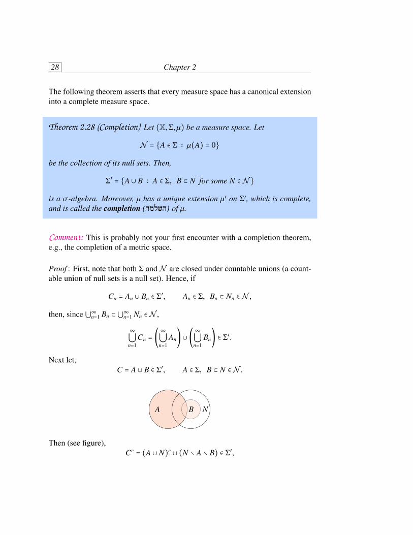
C = A ∪ B ∈ ⌃′, A ∈ ⌃, B ⊂ N ∈ N .
A B N
Then (see figure),Cc = (A ∪ N)c ∪ (N � A � B) ∈ ⌃′,
Measure spaces 29
proving that ⌃′ is indeed a �-algebra.—4h(2017)—
It is quite clear now to define the extended measure µ′(A ∪ B), as we must have
µ(A) = µ′(A) ≤ µ′(A ∪ B) ≤ µ′(A ∪ N) = µ(A ∪ N) ≤ µ(A) + µ(N) = µ(A),i.e.,
µ′(A ∪ B) = µ(A).We first need to show that this extension does not depend on the representation:let
A1 ∪ B1 = A2 ∪ B2,
where A1,A2 ∈ ⌃, B1 ⊂ N1 ∈ N and B2 ⊂ N2 ∈ N . Then,
A1 ⊂ A1 ∪ B1 = A2 ∪ B2 ⊂ A2 ∪ N2,
and by monotonicity,
µ(A1) ≤ µ(A2) + µ(N2) = µ(A2).By symmetry, µ(A1) = µ(A2).Now that we have shown that µ′ is well-defined, it is easy to see that it extends µ.For A ∈ ⌃,
A = A ∪�,where � ⊂ � ∈N , hence
µ′(A) = µ(A),namely, µ′�⌃ = µ.We next prove that µ′ is a measure, i.e., that it is �-additive. This follows from thefact that null sets are closed under countable unions. That is, if An is a sequenceof measurable sets, Bn ⊂ Nn ∈ N , and An ∪ Bn are disjoint, then
µ′ � ∞�n=1(An ∪ Bn)� = µ′ � ∞�
n=1An ∪ ∞�
n=1Bn� = µ� ∞�
n=1An� = ∞�
n=1µ(An) = ∞�
n=1µ′(An ∪ Bn).
We next prove that µ′ is complete. Let A ∈ ⌃ and B ⊂ N ∈ N satisfy
µ′(A ∪ B) = µ(A) = 0.
Then, A ∈ N and so is A ∪ N. If C ⊂ A ∪ B, then
C = �∪C ∈ ⌃′,
30 Chapter 2
proving that µ′ is complete.It remains to prove that the extension is unique. Let ⌫ be an extension of µ definedon ⌃′. For A ∈ ⌃ and B ⊂ N ∈ N ,
µ(A) = ⌫(A) ≤ ⌫(A ∪ B) ≤ ⌫(A ∪ N) ≤ ⌫(A) + ⌫(N) = µ(A) + µ(N) = µ(A),proving that ⌫(A ∪ B) = µ(A) = µ′(A ∪ B). n
2.3 Borel measures on R: a first attempt
Our ultimate goal is to define a measure µ on R satisfying
µ((a,b)) = b − a.
The measure µ has to be defined for all open segments, and as a result, it must bedefined at least for all sets in the �-algebra generated by the collection of opensegments. i.e., for all sets in the Borel �-algebra B(R).In this section we shall start developing such a measure. In fact, we shall startconstructing a more general family of Borel measures on the real line. The gener-alization is based on the following observation:
Proposition 2.29 Let (R,B(R), µ) be a measure space, such that µ is finite forevery finite interval. Consider the cumulative distribution function (-;%% ;*781&5�;9")7/% ;&#-5)
F(x) =�����������µ((0, x]) x > 00 x = 0−µ((x,0]) x < 0
(2.1)
Then,
(a) For every a < b,µ((a,b]) = F(b) − F(a).
(b) F is monotonically-increasing.(c) F is right-continuous (including at −∞).

Measure spaces 31
Comment: You may be familiar with the cumulative distribution function from aProbability course. The standard length measure on the real line corresponds tothe case F(x) = x.
Proof :
(a) For every 0 ≤ a < b, (a,b] = (0,b] � (0,a], hence
µ((a,b]) = µ((0,b]) − µ((0,a]) = F(b) − F(a).Likewise, for every a < 0 < b, (a,b] = (a,0] � (0,b], hence
µ((a,b]) = µ((a,0]) + µ((0,b]) = F(b) − F(a),and similarly for the case a < b < 0.
(b) The monotonicity of F follows from the monotonicity of µ.(c) Without loss of generality, assume that x ≥ 0. By the upper-semicontinuity
of µ (for sets of finite measure!), for every sequence xn ↘ x,
limn→∞F(xn) = lim
n→∞µ((0, xn]) = µ�∞�n=1(0, xn]� = µ((0, x]) = F(x).
The same argument works for x < 0 and x = −∞.
n
We will proceed in the reverse direction, and construct for every monotonically-increasing right-continuous function F, a Borel measure on the real line; this con-struction does not cover all possible Borel measures on the real line, but as weshall see, it covers all possible Borel measures that are finite on finite intervals.Thus far, given such a function F, we have a set-function for semi-open sets of theform (a,b]. Note that we may well let a and b assume the values ±∞. The mea-sure, of the semi-open intervals (−∞,b] and (a,∞]will be finite or not dependingon whether F has a finite limit at ±∞.Thus, we have an early notion of a set-function for all sets in the family
E = {�} ∪ {(a,b] ∶ −∞ ≤ a < b} ∪ {(a,∞) ∶ a ∈ R}.The reason for working with semi-open intervals is essentially technical, and re-lated to the following definition:
32 Chapter 2
Definition 2.30 LetX be an non-empty set. An elementary family (�;*$&2* %(5:/)of subsets of X, is a collection E of subsets of X (the elementary sets), satisfying
(a) � ∈ E .(b) E is closed under pairwise intersection (hence under finite intersection).(c) For every E ∈ E , Ec is a finite disjoint union of elementary sets; that is
∀E ∈ E , ∃n ∈ N, (Fk)nk=1 ⊂ E , such that Ec = n�k=1
Fk.
Example: The semi-open intervals are an elementary family of subsets of R. ▲▲▲An elementary family of sets is somewhat reminiscent of a subbase (�%7(/- 2*2")in a topological space, in that it is a basis for constructing an algebra, as shown bythe following proposition:
Proposition 2.31 Let E be an elementary family of subsets of X. Then, the col-lection of finite disjoint unions of elementary sets,
A = � n�k=1
Ek ∶ n ∈ N ∪ {0}, E1, . . . ,En ∈ E� ,is an algebra.
Proof : Clearly, � ∈ A. Next, A is closed under pairwise intersection: Let
A = n�k=1
Ek ∈ A and B = m�j=1
F j ∈ A,then
A ∩ B = n�k=1
m�j=1(Ek ∩ F j) ∈ A,
where we used the fact that E is closed under pairwise intersection. Finally, A isclosed under complementation: Let
A = n�k=1
Ek, where Eck = nk�
j=1Fk, j ∈ A.

Measure spaces 33
Then by Item (b),
Ac = n�k=1
Eck ∈ A.
n
The next step is to use monotonically-increasing, right-continuous functions F ∶R → R to construct a set-function on the algebra A. Measures, however, aredefined on �-algebras, which brings us to the following definition:
Definition 2.32 Let X be an non-empty set and let A be an algebra of subsets ofX. A function µ0 ∶ A → [0,∞] is called a pre-measure (�%$*/ .$8) if µ0(�) = 0and µ0 is �-additive. Note that the disjoint union of (En) ⊂ A is not necessarilyin A; however, if it is, then
µ0 � ∞�n=1
En� = ∞�n=1µ0(En).
Comment: While a pre-measure looks “almost” like a measure, its restriction to analgebra, rather than a �-algebra, makes it easier to construct, hence a convenientstarting point for constructing measures.
Proposition 2.33 Let F ∶ R → R be monotonically-increasing and right-continuous (including at −∞). Let A be the algebra of disjoint unions of semi-open intervals. Then, the set-function µ0 ∶ A → [0,∞] defined by µ0(�) = 0and
µ0(A) = n�j=1(F(bk) − F(ak)) for A = n�
k=1(ak,bk] (2.2)
is a pre-measure for A. (Note that one of the ak may be −∞.)
Proof : We will break the proof into a few lemmas. n
Lemma 2.34 The function µ0 defined by (2.2) is well-defined; it does not dependon the representation of elements in A.

34 Chapter 2
Proof : For example, suppose that
I ≡ (a,b] = n�k=1(ak,bk] ≡ n�
k=1Ik.
The (ak), (bk) can be re-ordered, such that
a = a1 < b1 = a2 < b2 = � = an < bn = b.
By the definition of µ0,
µ0 � n�k=1
Ik� = n�j=1(F(bk) − F(ak)) = F(bn) − F(a1) = µ0(I).
With some technical work, we may show that µ0 is uniquely-defined for any ele-ment of A. n—6h(2017)—
Lemma 2.35 The function µ0 defined by (2.2) is finitely-additive.
Proof : This is immediate. Let
A = n�i=1(ai,bi] and B = m�
j=1(c j,dj]
be disjoint finite disjoint unions of semi-open intervals. Then,
µ0(A � B) = n�i=1(F(bi) − F(ai)) + m�
j=1(F(dj) − F(c j)) = µ0(A) + µ0(B).
n
Lemma 2.36 LetI = (a,b] = ∞�
n=1(an,bn] = ∞�
n=1In,
thenµ0(I) = ∞�
n=1µ0(In).

Measure spaces 35
Proof : On the one hand, since for every n,
n�k=1
Ik ⊂ I,
and since µ0 is finitely-additive,
µ0 � n�k=1
Ik� = n�k=1µ0(Ik) ≤ µ0(I).
Letting n→∞, ∞�n=1µ0(In) ≤ µ0(I).
—6h(2018)—In the other direction, let " > 0 be given. Since F is right-continuous, there existsa � > 0 such that
F(a + �) − F(a) < ",i.e.,
µ0((a,a + �]) < ".Likewise, for every n ∈ N, there exists a �n > 0, such that
F(bn + �n) − F(bn) < "2n ,
namely.µ0((bn,bn + �n]) < "2n .
( ( ]][ )a an bn b
a + � bn + �n
The union, ∞�n=1(an,bn + �n)
is an open cover of the compact set [a+ �,b]. Thus, there exists a finite sub-cover,
m�k=1(ank ,bnk + �nk) ⊃ [a + �,b].

36 Chapter 2
By monotonicity,
µ0((a + �,b]) ≤ m�k=1µ0((ank ,bnk + �nk]).
By the definition of � and �k,
µ0(I) = µ0((a,a + �]) + µ0((a + �,b])≤ " + m�
k=1µ0((ank ,bnk + �nk])
≤ " + m�k=1�µ0((ank ,bnk]) + "2nk
�≤ " + ∞�
n=1�µ0((an,bn]) + "2n�
= 2" + ∞�n=1µ0(In).
Since " is arbitrary,
µ0(I) ≤ ∞�n=1µ0(In),
which completes the proof. n
Lemma 2.37 The function µ0 defined by (2.2) is �-additive.
Proof : Suppose that An ∈ A are disjoint, with
An = pn�k=1
In,k,
such that ∞�n=1
An = q�m=1
Jm ∈ A.We need to show that ∞�
n=1µ0(An) = q�
m=1µ0(Jm),

Measure spaces 37
i.e., that ∞�n=1
pn�k=1µ0(In,k) = q�
m=1µ0(Jm).
Now for every m = 1, . . . ,q,
∞�n=1
pn�k=1(Jm ∩ In,k) = Jm,
hence by the previous lemma,
∞�n=1
pn�k=1µ0(Jm ∩ In,k) = µ0(Jm).
Summing over m we recover the desired result. n
In conclusion, given any monotonically-increasing right-continuous function F,we have a pre-measure µ0, defined on the algebra A of finite disjoint unions ofsemi-open intervals. Moreover, �(A) =B(R). What is now missing is a methodfor extending pre-measures into measures. We undertake this task in the nextsection. This is not a trivial task, as �-algebras may be very large collections, forwhich we do not have an explicit representation.
2.4 Outer-measures
2.4.1 Definition
Definition 2.38 (outer-measure) Let X be a non-empty set. An outer-measure
(�;*1&7*( %$*/) on X is a function µ∗ ∶P(X)→ [0,∞] satisfying
(a) µ∗(�) = 0.(b) Monotonicity: if Y ⊂ Z then µ∗(Y) ≤ µ∗(Z).(c) Countable sub-additivity (�;*;**1/ ;&*"*)*$! ;;): for every sequence (Yn) ⊂
P(X),µ∗ �∞�
n=1Yn� ≤ ∞�
n=1µ∗(Yn).
Unlike measures, outer-measures, which are defined for all subsets of X, are easyto construct. The following proposition provides a canonical construction:

38 Chapter 2
Proposition 2.39 Let E ⊂ P(X) be a collection of sets including � and X, andlet ⇢ ∶ E → [0,∞] be a set function satisfying ⇢(�) = 0. Then,
µ∗(Y) = inf �∞�n=1⇢(En) ∶ En ∈ E , Y ⊂ ∞�
n=1En� (2.3)
is an outer-measure.
Proof : First, note that µ∗ is well-defined and non-negative, as the set
�∞�n=1⇢(En) ∶ En ∈ E , Y ⊂ ∞�
n=1En�
is non-empty (choose E1 = X, and Ei = � for all n ≥ 2). Also, µ∗(�) = 0 since wecan take En = � for all n. If Y ⊂ Z, then a covering of Z is also a covering of Y ,i.e.,
�(En) ⊂ E ∶ Y ⊂ ∞�n=1
En� ⊃ �(En) ⊂ E ∶ Z ⊂ ∞�n=1
En� ,which is an inclusion between sets of sequences. Hence,
�∞�n=1⇢(En) ∶ En ∈ E , Y ⊂ ∞�
n=1En� ⊃ �∞�
n=1⇢(En) ∶ En ∈ E , Z ⊂ ∞�
n=1En� ,
which is an inclusion between sets of numbers. The infimum of the left-hand sideis less or equal than the infimum of the right-hand side, i.e.,
µ∗(Y) ≤ µ∗(Z).It remains to show that µ∗ is countably sub-additive. Let (Yn) ⊂ P(X). Ifµ∗(Yn) = ∞ for some n, then there is nothing to prove. Otherwise, by the def-inition of µ∗(Yn), there exist for every " > 0, En,k ∈ E , such that
Yn ⊂ ∞�k=1
En,k and∞�
k=1⇢(En,k) < µ∗(Yn) + "2n .
Then, ∞�n=1
Yn ⊂ ∞�n=1
∞�k=1
En,k,

Measure spaces 39
and ∞�n=1
∞�k=1⇢(En,k) < ∞�
n=1µ∗(Yn) + ",
proving that
µ∗ �∞�n=1
Yn� ≤ ∞�n=1µ∗(Yn) + ".
Since " is arbitrary, µ∗ is countably sub-additive. n
Example: We can define an outer-measure on R by taking
E = {(a,b) ∶ a < b} ∪� ∪R,and setting ⇢((a,b)) = b − a, ⇢(�) = 0 and ⇢(R) = ∞. We will do something inthat spirit shortly. ▲▲▲ —7h(2018)—
2.4.2 Caratheodory’s theorem
We next follow the path of Caratheodory and show how an outer-measure maybe used to define a measure on a collection of measurable sets. (ConstantinCaratheodory (1873–1950) was a Greek mathematician who spent most of hisprofessional career in Germany.)
Definition 2.40 Let µ∗ be an outer-measure on X. A set A ⊂ X is called µ∗-measurable if
µ∗(Y) = µ∗(Y ∩ A) + µ∗(Y ∩ Ac) ∀Y ⊂ X.
AY
Y ∩ A Y ∩ Ac
Comment: By the sub-additivity of the outer-measure, it is always the case that
µ∗(Y) ≤ µ∗(Y ∩ A) + µ∗(Y ∩ Ac),

40 Chapter 2
hence A is µ∗-measurable if and only if
µ∗(Y) ≥ µ∗(Y ∩ A) + µ∗(Y ∩ Ac) ∀Y ⊂ X.Since this property holds trivially if µ∗(Y) =∞, it su�ces to verify it for µ∗-finitesets Y .
. Exercise 2.26 Let X be a non-empty set, and let
µ∗(Y) = �������0 Y = �1 otherwise.
(a) Show that µ∗ is an outer-measure. (b) Find all the µ∗-measurable sets.
Proposition 2.41 Let µ∗ be an outer-measure on X. Then, the collection
⌃ = {A ⊂ X ∶ A is µ∗-measurable}of all µ∗-measurable sets is a �-algebra, which we denote by �(µ∗).
Proof : We will proceed as follows:
(i) Show that ⌃ is non-empty, by showing that � ∈ ⌃.(ii) Show that A ∈ ⌃ implies that Ac ∈ ⌃,
(iii) Show that ⌃ is closed under finite union.(iv) Show that ⌃ is closed under countable union.
(i) For every Y ⊂ X,
µ∗(Y) = µ∗(Y ∩�)���������������������������������������µ∗(�)=0
+µ∗(Y ∩�c)���������������������������������������������µ∗(Y)
,
i.e., � ∈ ⌃.(ii) ⌃ is closed under complementation, since A and Ac play a symmetric role inthe definition of µ∗-measurability.(iii) Let A,B ∈ ⌃. We need to show that for every Y ⊂ X,
µ∗(Y) ≥ µ∗(Y ∩ (A ∪ B)���������������������������������������������������Y1�Y2�Y3
) + µ∗(Y ∩ (A ∪ B)c���������������������������������������������������������Y4
).

Measure spaces 41
A B
Y4
Y1 Y2Y3
Since A,B are µ∗-measurable,µ∗(Y) = µ∗(Y1 � Y2) + µ∗(Y3 � Y4)= µ∗(Y1) + µ∗(Y2) + µ∗(Y3) + µ∗(Y4)≥ µ∗(Y1 � Y2 � Y3) + µ∗(Y4),
where in the last passage we used the sub-additivity of µ∗.(iv) By Proposition 2.3, it su�ces to show that ⌃ is closed under countable disjointunions. Let (An) ⊂ ⌃ be a sequence of disjoint µ∗-measurable sets, and define
Bn = n�k=1
Ak and B = ∞�n=1
An.
A1 A2 An−1 An�Y
Let Y ⊂ X. Since An ∈ ⌃ for every n,
µ∗(Y ∩ Bn) = µ∗(Y ∩ Bn ∩ An) + µ∗(Y ∩ Bn ∩ Acn)= µ∗(Y ∩ An) + µ∗(Y ∩ Bn−1),
from which follows inductively that
µ∗(Y ∩ Bn) = n�k=1µ∗(Y ∩ Ak). (2.4)
By the closure of ⌃ under finite unions, Bn ∈ ⌃; it follows that for every n,
µ∗(Y) = µ∗(Y ∩ Bn) + µ∗(Y ∩ Bcn)
= n�k=1µ∗(Y ∩ Ak) + µ∗(Y ∩ Bc
n)≥ n�
k=1µ∗(Y ∩ Ak) + µ∗(Y ∩ Bc),
42 Chapter 2
where we used (2.4), replaced Bcn by the smaller Bc and used the monotonicity of
µ∗. Letting n→∞,
µ∗(Y) ≥ ∞�k=1µ∗(Y ∩ Ak) + µ∗(Y ∩ Bc). (2.5)
Finally, using again the countable sub-additivity of µ∗,
µ∗(Y ∩ B) = µ∗ �Y ∩ � ∞�n=1
An�� = µ∗ � ∞�n=1(Y ∩ An)� ≤ ∞�
k=1µ∗(Y ∩ Ak), (2.6)
showing thatµ∗(Y) ≥ µ∗(Y ∩ B) + µ∗(Y ∩ Bc),
i.e., B ∈ ⌃. n—8h(2017)—
. Exercise 2.27 Let µ∗ be an outer-measure on a set X. Let A,B ⊂ X, such that at least oneof them is µ∗-measurable. Prove that
µ∗(A) + µ∗(B) = µ∗(A ∪ B) + µ∗(A ∩ B).. Exercise 2.28 Let µ∗ be an outer-measure on X. Suppose that µ∗ is finitely-additive onP(X), i.e., for all disjoint A,B ⊂ X, µ∗(A � B) = µ∗(A) + µ∗(B). Show that �(µ∗) =P(X).
Theorem 2.42 (Caratheodory) Let µ∗ be an outer-measure on X. Then, the re-striction µ = µ∗��(µ∗) is a measure on (X,�(µ∗)). Moreover, this measure iscomplete.
Proof : The property µ(�) = 0 follows from the defining properties of outer-measures and the fact that � ∈ �(µ∗). To show that µ is �-additive, let (An) ⊂�(µ∗) be disjoint and let B = �∞n=1 An. We have just shown (see (2.5) and (2.6))that for every Y ⊂ X,
µ∗(Y) = ∞�k=1µ∗(Y ∩ Ak) + µ∗(Y ∩ Bc) = µ∗(Y ∩ B) + µ∗(Y ∩ Bc).
Substituting Y = B and using the fact that µ∗��(µ∗) = µ,µ(B) = µ∗(B) = ∞�
k=1µ∗(B ∩ Ak) + µ∗(B ∩ Bc) = ∞�
k=1µ(Ak).

Measure spaces 43
It remains to show that µ is complete, i.e., that �(µ∗) contains every subset ofevery µ-null set. Let N ∈ �(µ∗) satisfy µ(N) = 0 and let A ⊂ N. By the sub-additivity and the monotonicity of the outer-measure, for every Y ⊂ X,
µ∗(Y) ≤ µ∗(Y ∩ A) + µ∗(Y ∩ Ac) ≤ µ∗(N) + µ∗(Y) = 0 + µ∗(Y),i.e., A is µ∗-measurable. n
To summarize, we may construct a measure onX as follows: take any collection Eof sets including � and X, along with a function ⇢ ∶ E → [0,∞], which only needsto vanish on the empty set. Then, construct an outer-measure µ∗ via formula(2.3). The outer-measure defines a �-algebra of µ∗-measurable sets, �(µ∗). Therestriction of µ∗ to this �-algebra is a complete measure. —8h(2018)—
. Exercise 2.29 Let µ∗ be an outer-measure on X, and let µ = µ∗��(µ∗) be the induced com-plete measure on the �-algebra of µ∗-measurable sets. Let ⌫∗ be the outer-measure defined by(2.3), with E = �(µ∗) and ⇢ = µ, namely,
⌫∗(Y) = inf �∞�n=1µ(En) ∶ En ∈ �(µ∗), Y ⊂ ∞�
n=1En� .
(a) Prove thatµ∗(Y) ≤ ⌫∗(Y) ∀Y ⊂ X.
(b) Prove that µ∗(Y) = ⌫∗(Y) if and only if there exists an A ∈ �(µ∗), such that Y ⊂ A andµ∗(Y) = µ(A).The following proposition asserts that if one starts with a �-finite measure µ,constructs from it an outer-measure µ∗, and proceeds to derive a measure µ usingCaratheodory’s theorem, then one obtains the closure of the original measure.
Proposition 2.43 Let (X,⌃, µ) be a �-finite measure space. Let µ∗ be the outer-measure induced by µ. We denote by µ the restriction of µ∗ to �(µ∗). Prove that(X,�(µ∗), µ) is the completion of (X,⌃, µ). That is, all the sets A ∈ �(µ∗) are ofthe form
A = B ∪ Y,
where B ∈ ⌃ and Y ⊂ N with µ(N) = 0.
. Exercise 2.30 Prove Proposition 2.43.

44 Chapter 2
2.4.3 Extension of pre-measures
Thus far, we have the following construction:
(E ,⇢)A set function
(P(X), µ∗)An outer-measure
(�(µ∗), µ∗��(µ∗))A complete measure
Note that it is not clear a priori which measure µ results from a given set function⇢. A useful construction would start from a clever choice of set function ⇢, bytaking E su�ciently large and ⇢ satisfying properties expected for µ.In this section, we show how to use Caratheodory’s theorem to extend a pre-measure defined on an algebra A into a measure on the �-algebra �(A). In par-ticular, this will complete the construction of Borel measures on R with givencumulative distribution function F.
Proposition 2.44 LetA be an algebra of subsets ofX and let µ0 be a pre-measureon A. Let µ∗ be the outer-measure defined by
µ∗(A) = inf �∞�n=1µ0(En) ∶ En ∈ A, A ⊂ ∞�
n=1En� .
Then,
(a) µ∗�A = µ0.
(b) Every set in A is µ∗-measurable, i.e., A ⊂ �(µ∗).
Comment: Since A is an algebra, we can replace any sequence En from a disjointsequence Fn, such that ∞�
n=1Fn = ∞�
n=1En.
Since by monotonicity, ∞�n=1µ0(Fn) ≤ ∞�
n=1µ0(En),
such a substitution does not change the infimum.
Measure spaces 45
Proof : (a) Let A ∈ A. Setting E1 = A and En = � for n > 1,
A ⊂ ∞�n=1
En and∞�
n=1µ0(En) = µ0(A),
i.e.,µ∗(A) ≤ µ0(A).
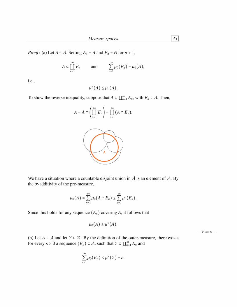
To show the reverse inequality, suppose that A ⊂�∞n=1 En, with En ∈ A. Then,
A = A ∩ � ∞�n=1
En� = ∞�n=1(A ∩ En).
A
We have a situation where a countable disjoint union in A is an element of A. Bythe �-additivity of the pre-measure,
µ0(A) = ∞�n=1µ0(A ∩ En) ≤ ∞�
n=1µ0(En).
Since this holds for any sequence (En) covering A, it follows that
µ0(A) ≤ µ∗(A).—9h(2017)—
(b) Let A ∈ A and let Y ⊂ X. By the definition of the outer-measure, there existsfor every " > 0 a sequence (En) ⊂ A, such that Y ⊂�∞n=1 En and
∞�n=1µ0(En) < µ∗(Y) + ".

46 Chapter 2
Since µ0 is �-additive on A,
µ∗(Y) + " > ∞�n=1µ0(En)
= ∞�n=1(µ0(En ∩ A) + µ0(En ∩ Ac))
= ∞�n=1µ∗(En ∩ A) + ∞�
n=1µ∗(En ∩ Ac)
≥ µ∗ � ∞�n=1
En ∩ A� + µ∗ � ∞�n=1
En ∩ Ac�≥ µ∗(Y ∩ A) + µ∗(Y ∩ Ac),
where the passage to the second line follows form the fact that A,En ∈ A, thepassage to the third line follows from µ∗�A = µ0 and the passage to the fourth linefollows from the sub-additivity and monotonicity of µ∗. Since " is arbitrary, itfollows that A is µ∗-measurable. n
Theorem 2.45 (Extension of a pre-measure) LetA be an algebra of subsets of Xand let µ0 be a pre-measure on A; let µ∗ be the outer-measure induced by µ0.Then,
(a) µ = µ∗��(A) is a measure on �(A) extending µ0.
(b) If ⌫ is some other measure on �(A) extending µ0, then
⌫(A) ≤ µ(A),(c) ⌫(A) = µ(A) for all µ-finite sets.
(d) If µ0 is �-finite, then the extension is unique.
Proof : (a) By Proposition 2.44, A ⊂ �(µ∗), hence
�(A) ⊂ �(µ∗).Since
µ∗��(µ∗) is a (complete) measure,

Measure spaces 47
and since the restriction of a measure on a sub-�-algebra is a measure, it followsthat
µ = µ∗��(A) is a measure.
Since µ∗ extends µ0, so does µ.(b-c) Next, let ⌫ be a measure on �(A) extending µ0. If µ(A) = ∞ then theassertion ⌫(A) ≤ µ(A) is trivial. Otherwise, let A ∈ �(A) be µ-finite. Sinceµ(A) = µ∗(A), there exists for every " > 0 a sequence En ∈ A such that A ⊂�∞n=1 En, and ∞�
n=1µ0(En) < µ∗(A) + " = µ(A) + ".
(This is where we used the finiteness of µ(A).) On the other hand, by the sub-additivity of ⌫,
⌫(A) ≤ ∞�n=1⌫(En) = ∞�
n=1µ0(En),
proving that ⌫(A) ≤ µ(A).For the reverse inequality, set
E = ∞�n=1
En.
By the countable additivity of the measure,
µ(E) = ∞�n=1µ0(En) ≤ µ(A) + ",
henceµ(E) − µ(A) ≤ ".
By the �-additivity of the measures µ and ⌫, and the fact that µ and ⌫ coincide onA,
⌫(E) = ∞�n=1⌫(En) = ∞�
n=1µ(En) = µ(E).
It follows that
µ(A) ≤ µ(E) = ⌫(E) = ⌫(A) + ⌫(E � A) ≤ ⌫(A) + µ(E � A) ≤ ⌫(A) + ",proving that µ(A) = ⌫(A).

48 Chapter 2
(d) Finally, suppose that µ0 is �-finite, i.e.,
X = ∞�n=1Xn,
with Xn ∈ A and µ0(Xn) <∞; without loss of generality we may assume that theXn are disjoint. Then, for every A ∈ �(A),
µ(A) = ∞�n=1µ(A ∩Xn) = ∞�
n=1⌫(A ∩Xn) = ⌫(A).
n
. Exercise 2.31 Let µ∗ be an outer-measure onX induced by a pre-measure µ0 on an algebraA. Suppose that E is µ∗-measurable, and there exist A,B ⊂ X, such that E = A � B and
µ∗(E) = µ∗(A) + µ∗(B).Prove that A,B are both µ∗-measurable.
. Exercise 2.32 Let A be an algebra of sets of X. Let A� be the collection of countableunions of sets in A, and let A�� be the collection of countable intersections of sets in A�. Let µ0be a pre-measure on A and let µ∗ be the induced outer-measure.
(a) Show that for every Y ⊂ X and " > 0, there exists an A ∈ A�, such that Y ⊂ A and
µ∗(A) ≤ µ∗(Y) + ".(b) Show that if µ∗(E) <∞, then E is µ∗-measurable if and only if there exists for every " > 0
a B ∈ A��, such that E ⊂ B and µ∗(B � E) < ".(c) Show that the restriction µ∗(E) <∞ in (b) is not needed if µ0 is �-finite.
. Exercise 2.33 Let µ∗ be an outer-measure on X induced from a pre-measure µ0 on an al-gebraA, and let µ = µ∗��(µ∗) be the induced complete measure on the �-algebra of µ∗-measurablesets. Let µ∗∗ be the outer-measure defined by (2.3), with E = �(µ∗) and ⇢ = µ, namely,
µ∗∗(Y) = inf �∞�n=1µ(En) ∶ En ∈ �(µ∗), Y ⊂ ∞�
n=1En� .
Prove thatµ∗(Y) = µ∗∗(Y) ∀Y ∈ X,
In other words, µ0 and µ induce the same outer-measure, and as a result, if one starts with a pre-measure the process of extracting a measure cannot be further iterated to yield another measure.(Note that this exercise di↵ers from Ex. 2.29 in that µ∗ is induced by a pre-measure.)

Measure spaces 49
To conclude, we have the following picture:
µ0 defined onan algebra A µ∗ defined on
P(X) µ defined on�(A)
µ∗ defined onP(X)µ defined on
�(µ∗)The fact that µ induces the same outer-measure µ∗ as the one that generated it wasproved in Ex. 2.33. Finally, by Proposition 2.43, the complete measure µ is thecompletion of µ.
. Exercise 2.34 Let µ0 be a finite pre-measure on (X,⌃), and let µ∗ be the induced outer-measure. For Y ⊂ X, we define its inner-measure ( �;*/*15 %$*/),
µ∗(Y) = µ0(X) − µ∗(Yc).Prove that A ∈ �(µ∗) if and only if its outer-measure coincides with its inner-measure.
2.5 Measures on R
2.5.1 Borel measures on the real line
We may now combine together the construction of the pre-measures induced bya monotonically-increasing, right-continuous function F and Caratheodory’s the-orem applied by pre-measures (Theorem 2.45). Then, we will focus our attentionon the standard Lebesgue measure, which corresponds to the choice of F(x) = x. —10h(2017)—
Proposition 2.46 (a) Let F ∶ R → R be monotonically-increasing and right-continuous. Then, F defines a unique Borel measure, denoted µF, on R, suchthat
µF((a,b]) = F(b) − F(a).

50 Chapter 2
(b) Conversely, every Borel measure µ on R, which is finite on all bounded Borelsets, is of the form µ = µF, where
F(x) =�����������µ((0, x]) x > 00 x = 0−µ((x,0]) x < 0.
(2.7)
Proof : (a) By Proposition 2.33, F defines a pre-measure µ0 on A. By the exten-sion Theorem 2.45, µ0 extends to a measure on �(A) = B(R), i.e., into a Borelmeasure µF . Moreover, this measure is �-finite, as
R = ∞�n=−∞(n,n + 1] and µ0((n,n + 1]) = F(n + 1) − F(n) <∞.
(b) Given a Borel measure µ and defining F as in (2.7), we obtain that µ and µF
agree on semi-open intervals, hence on A. By the uniqueness of the extension,they are equal n
The measure µF is not complete. Its completion, �F , which equals µ∗F �⌃F , where⌃F = �(µ∗F), and µ∗F is induced by µF , is called the Lebesgue-Stieltjes measureassociated with F.We proceed to study regularity properties of the family of Borel measures µF onR;
Lemma 2.47 Let (R,B(R), µF) be a Borel measure. For every A ∈B(R),µF(A) = inf �∞�
n=1µF((an,bn]) ∶ A ⊂ ∞�
n=1(an,bn]� .
Proof : This is an immediate consequence of the the definition of the outer-measureµ∗F , which is generated by the pre-measure µ0 on the algebra of finite unions ofsemi-open intervals, and the fact that µF and µ0 coincide for semi-open intervals.n
Measure spaces 51
Lemma 2.48 Every open interval on R is a countable disjoint union of semi-openintervals. In particular,
�∞�n=1µF((an,bn]) ∶ A ⊂ ∞�
n=1(an,bn]� ⊃ �∞�
n=1µF((an,bn)) ∶ A ⊂ ∞�
n=1(an,bn)�
Proof : Clearly,
(a,b) = ∞�k=1(ak,bk],
where a1 = a and bk ↗ b. Using the same notation, if
A ⊂ ∞�n=1(an,bn),
thenA ⊂ ∞�
n=1
∞�k=1(ak
n,bkn],
and ∞�n=1
∞�k=1µF((ak
n,bkn]) = µF((an,bn)),
proving the second part. n
Lemma 2.49 Let (R,B(R), µF) be a Borel measure. For every A ∈B(R),µF(A) = inf �∞�
n=1µF((an,bn)) ∶ A ⊂ ∞�
n=1(an,bn)� ,
i.e., the semi-open intervals have been replaced by open intervals.
Proof : For A ∈B(R), denote
⌫(A) = inf �∞�n=1µF((an,bn)) ∶ A ⊂ ∞�
n=1(an,bn)� .

52 Chapter 2
It follows from Lemma 2.48 that
µF(A) ≤ ⌫(A).Conversely, let A ∈ B(R) and let " > 0. By definition, there exist (an,bn], suchthat
A ⊂ ∞�n=1(an,bn] and
∞�n=1µF((an,bn]) ≤ µF(A) + ".
Since F is right-continuous, there exists for every n a �n > 0, such that
F(bn + �n) − F(bn) < "2n ,
i.e.,µF((an,bn + �n)) ≤ µF((an,bn + �n]) ≤ µF((an,bn]) + "2n .
Then,A ⊂ ∞�
n=1(an,bn + �n),
and by the definition of ⌫ as an infimum,
⌫(A) ≤ ∞�n=1µF((an,bn + �n)) ≤ ∞�
n=1µF((an,bn]) + " ≤ µF(A) + 2".
Since this holds for every " > 0, we obtain
⌫(A) ≤ µF(A),which completes the proof. n—10h(2018)—
Proposition 2.50 Let µF be a Borel measure on R (as usual, finite on boundedintervals). Then,
(a) µ is outer-regular,
µF(A) = inf{µF(U) ∶ U ⊃ A is open}.(b) µ is inner-regular,
µF(A) = sup{µF(K) ∶ K ⊂ A is compact}.
Measure spaces 53
Comment: In the general context of Borel measures, a measure that is locally-finite (every point has a neighborhood having finite measure), inner- and outer-regular is called a Radon measure. What we are thus proving is that every locally-finite Borel measure on R is a Radon measure. Radon measures play an importantrole in functional analysis.
Proof :
(a) By Lemma 2.49, there exist for every " > 0 open intervals (an,bn), such that
A ⊂ ∞�n=1(an,bn) and
∞�n=1µF((an,bn)) ≤ µF(A) + ".
Setting U = �∞n=1(an,bn), and using the countable sub-additivity of the mea-sure µF ,
µF(U) ≤ ∞�n=1µF((an,bn)) ≤ µF(A) + ",
from which we deduce that
inf{µF(U) ∶ U ⊃ A is open} ≤ µF(A).The other direction is trivial, as A ⊂ U implies µF(A) ≤ µF(U) = µF(U).
(b) Suppose first that A is bounded. If it is closed, then it is compact, and thestatement is trivial. Otherwise, for " > 0, there exists by the first part anopen set U ⊃ A � A, such that
µF(U) ≤ µF(A � A) + ".Let K = A �U. It is compact, contained in A, and
µF(K) = µF(A) − µF(U) ≥ µF(A) − µF(A � A) − " = µF(A) − ",and this since holds for all " > 0,
sup{µF(K) ∶ K ⊂ A is compact} ≥ µF(A).The reverse inequality is once again trivial.
Remains the case where A is not bounded. Let
Aj = A ∩ ( j, j + 1], j = . . . ,−2,−1,0,1,2, . . . .

54 Chapter 2
By the result for bounded sets, there exists for every " > 0 a compact setKj ⊂ Aj, such that
µF(Kj) > µF(Aj) − 2−� j�"3.
Set
Hn = n�j=−n
Kj.
The Hn are compact and
Hn ⊂ ∞�j=−∞
Kj ⊂ ∞�j=−∞
Aj = A.
On the other hand,
µF(Hn) = n�j=−nµF(Kj) > µF � n�
j=−nAk� − ".
Letting n to infinity, we obtain that
limn→∞µF(Hn) ≥ µF(A) − ",
and since " is arbitrary, we obtain the desired result.
n
Finally, we use the above regularity result to show that modulo sets of measurezero, all the Borel sets on R are of relatively simple form:
Theorem 2.51 Let (R,B(R), µF) by a Borel measure. Then every Borel set A ∈B(R) can be represented in either way:
(a) A = B � N, where B is a G� set and µ(N) = 0.
(b) A = B ∪ N, where B is an F� set and µ(N) = 0.
. Exercise 2.35 Prove Theorem 2.51.

Measure spaces 55
2.5.2 The Lebesgue measure on R
The Lebesgue measure (�#⌥=�- ;$*/) on R is the complete measure generated bythe function F(x) = x. We denote it by m; the �-algebra is denoted by L and itselements are called Lebesgue-measurable (�#⌥=�- ;&$*$/). That is,
m((a,b]) = b − a.
With a certain abuse of notation, we also denote by m the Borel measure inducedby F(x) = x and call it Lebesgue measure as well. Generally, we will keep work-ing with the incomplete Borel measure, unless stated otherwise.By the definition of the outer-measure µ∗, for every A ∈B(R) (or every A ∈ L),
m(A) = inf �∞�n=1(bn − an) ∶ A ⊂ ∞�
n=1(an,bn]� .
Proposition 2.52 Every singleton has Lebesgue measure zero.
Proof : For every x ∈ R,
m({x}) = m�∞�n=1(x − 1�n, x]� = lim
n→∞m ((x − 1�n, x]) = limn→∞
1n= 0,
where in the second inequality we used the upper-semicontinuity of the measure.n
Corollary 2.53 Every countable set has Lebesgue measure zero.
. Exercise 2.36 Let N be a null set of (R,B(R),m). Prove that Nc is dense in R.
The following theorem shows that the Lebesgue measure satisfies natural invari-ance properties:
56 Chapter 2
Theorem 2.54 For ↵ ∈ R and � > 0, denote the a�ne transformation
T↵,�(x) = ↵x + �.Then,
T↵,�(B(R)) =B(R),and for evert A ∈B(R),
m(T↵,�(A) = ↵m(A).
Proof : If is easy to see that T↵,�(B(R)) is a �-algebra containing all the opensegments, hence
T↵,�(B(R)) ⊂B(R).Since this holds for every ↵,�, It follows that
B(R) = T1�↵,−��↵ (T↵,�(B(R))) ⊂ T↵,�(B(R)).Next, define
⌫(A) = ↵m(T−1↵,�(A)).
It is easy to see that ⌫ is a measure on B(R): indeed,
⌫(�) = ↵m(�) = 0,
and for disjoint An ∈B(R),⌫� ∞�
n=1An� = ↵m�T−1
↵,� � ∞�n=1
An�� = ↵m� ∞�n=1
T−1↵,�(An)� = ↵ ∞�
n=1m(T−1
↵,�(An)) = ∞�n=1⌫(An).
Furthermore, every every semi-open segment,
⌫((a,b]) = ↵m ((a − �)�↵, (b − �)�↵]) = m((a,b]).If follows that ⌫ and m are equal on the algebra of finite unions of semi-opensegments, and by the uniqueness of the extension ⌫ = m, or
m(A) = ↵,m(T−1↵,�(A)).
This completes the proof. n

Measure spaces 57
. Exercise 2.37 Prove that Theorem 2.54 remains valid if (R,B(R),m) is replaced by (R,L,m).
. Exercise 2.38 Let A ∈ L satisfy 0 < m(A) <∞. Prove that there exists for every ↵ ∈ (0,1)an open interval I, such that
↵m(I) ≤ m(A ∩ I) ≤ m(I). Exercise 2.39 Let A ⊂ E ⊂ B ⊂ R, such that A,B are Lebesgue-measurable and m(A) =m(B). Prove that E is Lebesgue-measurable.
Proof : SinceE � A ⊂ B � A
and m(B � A) = 0, it follows that E � A is measurable, hence so is
E = A ∩ (E � A).. Exercise 2.40 Let A ⊂ R be Lebesgue-measurable, with m(A) > 0. Prove that
A − A = {x − y ∶ x ∈ A, y ∈ A}contains a non-empty open segment.
. Exercise 2.41 Let A ⊂ R be of positive Lebesgue measure. Prove that A contains twopoints whose di↵erence is rational; same for irrational.
. Exercise 2.42 Let µ be a locally-finite Borel measure on R (every point is in an opensegment of finite measure) which is invariant under translation. Prove that µ is proportional to thestandard Borel measure m.
. Exercise 2.43 Let A be a Lebesgue-measurable set in R, such that m(A) = 1. Show that Ahas a subset having measure 1�2.
2.5.3 Measure and topology
The concept of a measure is intuitively associated with the size of a set. Thereare also set-theoretical notions of magnitude (cardinality), as well as topologicalnotions of magnitude: for example, sets that are both open and dense are usuallyconsidered to be “large”. As we will see, the topological notion of magnitude andthe measure-theoretic notion of magnitude are not always consistent.As we have seen (Proposition 2.52), every singleton in R has Lebesgue measurezero. It follows that Q, which is a countable union of singletons, has Lebesguemeasure zero. On the other hand,
m([0,1] �Q) = m([0,1]) −m([0,1] ∩Q) = 1.

58 Chapter 2
Thus, in this example of rationals versus irrationals, the two notions of magnitudecoincide.Let (rn) be an enumeration of the rationals in [0,1], and let In be an open intervalcentered at rn of length "�2n, where 0 < " < 1. Then,
U = �∞�n=1
In� ∩ (0,1)is open and dense in [0,1]. On the other hand, by the sub-additivity of the mea-sure,
m(U) ≤ ∞�n=1
m(In) = ∞�n=1
"
2n = ".Thus, open and dense sets in [0,1] can have arbitrarily small Lebesgue measure.In contrast, set
K = [0,1] �U.
Then, K is closed and nowhere dense, and yet
m(K) = m([0,1]) −m(U) ≥ 1 − ",showing that closed and nowhere dense sets in [0,1] can have Lebesgue measurearbitrarily close to 1.Note that there are no open intervals having Lebesgue measure zero, however,there are Lebesgue-null sets having the cardinality of the continuum, as the fol-lowing example shows. Recall that the Cantor set C, is the subset of [0,1] con-sisting of those numbers whose base-3 expansion contains only the digits 0 and2. It can be constructed inductively, by first removing from [0,1] the segment[1�3,2�3], then removing from each of the two remaining segments their mid-third, i.e., removing 2 segments of length 1�9, then 4 segments of length 1�27,and so on.

Measure spaces 59
The Cantor set has the cardinality of the continuum, since we can map bijectivelya base-3 expansion using the digits 0 and 2 to a base-2 expansion using the digits0 and 1, i.e., the Cantor set can be mapped bijectively to the unit segment.
Proposition 2.55 The Cantor set C is measurable and has measure zero.
Proof : The Cantor set can be represented as
C = [0,1] � ��∞�
n=1
2n−1�k=1
In,k�� ,
where m(In,k) = 1�3n. C is clearly measurable. Moreover,
m(C) = 1 − ∞�n=1
2n−1
3n = 1 − 13
11 − 2�3 = 0.
n —11h(2018)—
. Exercise 2.44 A set A ⊂ R is called a G�-set if it is a countable intersection of open sets (re-call that a dense G� set is called residual (�%1/: %7&"8)). Show that there exists a G� set containingall the rationals (i.e., a residual set) having Lebesgue measure zero.
. Exercise 2.45 Find two measurable sets A,B ∈ B(R), such that m(A) = m(B) = 0 andm(A + B) > 0, where
A + B = {a + b ∶ a ∈ A b ∈ B}.Finally, we have an argument showing that there exist Borel-measurable sets thatare not Lebesgue-measurable.
Proposition 2.56 L is strictly larger than B(R).
Proof : W asserted (without a proof) that the cardinality of B(R) is that of thecontinuum,
card(B(R)) = 2ℵ0 .
The cardinality if the Cantor set is also 2↵0 , and since it has measure zero, all itssubsets must be in L, i..e, L has the a cardinality larger than that of the continuum.n —12h(2017)—