Embed Size (px)
Citation preview

9
CHAPTER 2
LITERATURE SURVEY OF SELECTIVE HARMONIC
ELIMINATION TECHNIQUES
2.1 HARMONICS IN POWER SYSTEMS
Power system harmonics are power quality issues and harmonic
distortion is a representative of power quality problems which receives
continuous attention in the recent years and was dealt by Bollen (2003),
Choudhury (2001), Heydt (1998), (2001), Mack and Santoso (2001), Narain
(1995). Under electric power quality, voltage quality has become one of the
most important issues to be considered for electric suppliers to end users.
The usage of power electronic equipments has been increased in
recent years in industrial and consumer applications. Such loads draw the
non-linear sinusoidal current and voltage from the source (Wagner 2003).
These non-linear loads change the sinusoidal nature of the alternating current,
thereby resulting in the flow of harmonic currents in the AC power system.
The voltage and current waveforms are pure sinusoidal when the electric load
is linear. When the load is non-linear, the voltage and current waveforms are
quite often distorted. These non-linear loads change the sinusoidal nature of
alternating currents and results in flow of harmonic currents in power
systems. This deviation from perfect sine wave is to be represented as
harmonics.
These harmonics draw the non-linear sinusoidal current and voltage
from the source. Harmonics are caused by non-linear operation of devices,

10
such as power converters, arc-furnaces, and gas discharge lighting devices.
These devices have non-linear voltage-current characteristic meaning that the
current signal is not proportional to the applied voltage.
In recent years, the power quality issues in the utility grids have
received considerable attention to suppress harmonics related problems
resulting from a proliferation of non-linear loads. This has led to restricted
norms regarding utility power quality standards. As a result, a number of
research works are directed to fulfill these requirements by eliminating the
power quality degradation problems. The major reasons for power quality
degradation are as follows.
1. The modern devices and equipments being used by industrial
and commercial customers are more sensitive to power quality
variations than equipments used in the past.
2. An increasing number of power electronic devices are being
utilised to protect customers from power quality issues or acts
as an important part of energy transfer systems. Their
non-linear characteristics cause harmonic current which
results in additional heat in power system equipment,
interference with communication systems, and malfunctioning
of controls.
3. There is an increasing emphasis on overall power system
efficiency which causes a continuous growth in the application
of shunt capacitors for power factor correction. These
capacitors change the system impedance vs frequency
characteristic, resulting in resonance which can magnify
transient disturbances and harmonic distortion levels.

11
The major power disturbances which frequently appear in power
systems are divided into two categories based on the duration of occurrence.
They are transient problems and static problems. Transient problems include
voltage sags, voltage swells, electrical noise, and momentary interruption.
The duration of transient power quality problems varies from few
milliseconds to several seconds. Static problems include harmonics, outage,
under/over voltage, and impulses. The duration of static power quality
problems changes from several seconds to several minutes or even longer.
2.2 SOURCES AND EFFECTS OF HARMONIC DISTORTION
Harmonics are destruction phenomenon which causes enormous
amount of energy loss in transmission and distribution systems. The impact of
harmonics on the quality of electrical power continues to be a critical concern
for industrial and commercial users. According to Bennett et al (1997),
Brozek (1990), Henderson and Rose (1994), Purkayastha and Savoie (1990),
harmonics have significant impacts on generation units, transmission
equipments and customer facilities. The harmonic current flowing through the
energy transform/transfer devices generate excess heat, reduce the
transmission efficiency and shorten the device lifetime.
2.2.1 Sources of Harmonics
One common source of harmonics is iron core devices like
transformer. The magnetic characteristics of iron are almost linear over a
certain range of flux density, but quickly saturates as the flux density
increases. This non-linear magnetic characteristic is described by a hysteresis
curve. The non-linear hysteresis curve produces a non-sinusoidal excitation
current.

12
Core iron is not the only source of harmonics, but the generator also
themselves produce some 5th harmonic voltages due to magnetic flux
distortions, that occur near the stator slots and non-sinusoidal flux distribution
across the air gap. Other producers of harmonics include non-linear loads like
rectifiers, inverters, adjustable speed motor drives, welders, arc furnaces,
voltage controllers, and frequency converters.
Semiconductor switching devices produce significant harmonic
voltages as they abruptly chop voltage waveforms during their transition
between conducting and cut-off states. Inverter circuits are notorious for
producing harmonics, and are used widely today. An adjustable speed motor
drive is one application that makes use of inverter circuits, often using pulse
width modulation synthesis to produce the ac output voltage. Various
synthesis methods produce different harmonic spectra. Regardless of the
method used to produce an AC output voltage from a DC input voltage,
harmonics will be present on both sides of the inverter and must often be
mitigated.
2.2.2 Effects and Negative Consequences
The effects of three-phase harmonics on circuits are similar to the
effects of stress and high blood pressure on the human body. High levels of
stress or harmonic distortion can lead to problems for the utility's distribution
system, plant distribution system and any other equipment serviced by that
distribution system. Ambro et al (2003), Irene Yu-Hua and Emmanouil (2003)
have enumerated the effects of harmonics and that range from spurious
operation of equipment to a shutdown of important plant equipment, such as
machines or assembly lines. Harmonics leads to power system inefficiency.
Some of the negative consequences of harmonics on plant equipments are
listed below:

13
1. Conductor overheating is a function of the square RMS
current per unit volume of the conductor. Harmonic currents
on undersized conductors or cables cause a “skin effect”, which
increases with frequency and is similar to centrifugal force.
2. Capacitors can be affected by increase in heat rise leads to
power loss and reduced life on the capacitors. If a capacitor is
tuned to one of the characteristic harmonics such as the 5th or 7th,
overvoltage and resonance cause dielectric failure or rupture
of capacitor.
3. Harmonics cause false or spurious operations on fuses, circuit
breakers and trips, damaging or blowing components for no
apparent reason was mentioned by Brozek (1990).
4. Transformers have increased iron and copper losses or eddy
currents due to stray flux losses. This causes excessive
overheating in the transformer windings was explained by
Henderson and Rose (1994).
5. George (2003), Watson and Arrillaga (2003) have discussed
problems related to generators. Sizing and coordination is
critical to the operation of the voltage regulator and controls.
Excessive harmonic voltage distortion will cause multiple zero
crossings of the current waveform. Multiple zero crossings
affect the timing of the voltage regulator, causing interference
and operation instability.
6. Utility meters may record measurements inaccurately,
resulting in higher billings.
7. Harmonics cause failure of the commutation circuits, found in
DC drives and AC drives with silicon controlled rectifiers.
8. Computers/telephones may experience interference or failures.

14
2.3 INTERNATIONAL HARMONIC STANDARDS
The study of the effect of the harmonic distortion has lead to the
development of standards to limit its magnitude in order to prevent damage on
equipment and on the power system itself. After considering the effects and
damages due to harmonic distortion, the international standards were
introduced to supervise harmonic distortion issues. IEEE standard 519-1992
and IEC standard 61000-4-7 are the main international standards for
measurement and analysis of harmonics in power systems. These standards
used for specifying harmonic distortion is mainly divided into two types:
1. Load side standards: These are the standards which are used to
restrict the harmonic components coming out of the
experiments. These standards were mentioned in IEC-555 by
Simith (1992).
2. System side standards: These are the standards which are used
to limit harmonics in electric power supply or at the point of
common coupling. These standards were mentioned in IEEE
Standard 519-1992.
In 1969 the harmonic related standards were introduced. IEC
(International Electrotechnical Commission) and CENELEC (European
Committee for Electrotechnical Standardization) committees were formed to
investigate the effects of harmonic distortion in case of home appliances. The
CENELEC and IEC came with two harmonic distortion standards namely
EN 50006 and IEC 555 in the year 1975 and 1982 respectively. Germany was
the first country to use IEC 555 after EN 50006 standard from 1982 because
of its more comprehensive nature. Then the IEC 555 was updated as IEC 555-2,
which was then agreed by CENELEC to be EN 60555-2 European standard

15
was described in the year 1987. IEC 555-2 standard was updated and named
as IEC 1000-3-2 in the year 1995 by Finlay (1991). IEC 1000-3-2 had great
scope of applicability over IEC 555-2 it cover all equipments up to
16 Ampere per phase. According to the updated standards these equipments
fall under any one of the four categories.
1. Class A: The equipment which comes under class A category
are balanced three phase equipment and equipment not falling
into another category.
2. Class B: The equipment which comes under class B category
is portable and similar tools.
3. Class C: The equipment which comes under class C category
is lighting equipment, including dimmer controls.
4. Class D: The equipment which comes under class D category
are equipments having an input current with a “special wave
shape”.
This standard also stipulates the maximum allowable harmonic
distortion allowed in the voltage and current waveforms on various types of
systems. Most of the general equipment comes under class A and the
applicable limits for this are given in Table 2.1, all the units are expressed in
absolute amps. Similarly the limits for class B, class C and class D
equipments are given in the Tables 2.2-2.4 respectively. The limits specified
in the table are very important in order to improve power supply design and to
reduce problem in equipments.

16
Table 2.1 Harmonic current limits for class A equipment and certain
class C equipment with phase controlled lamp dimmers
(IEC 555-2)
Harmonicorder “n”
Maximum permissible harmoniccurrent (in amperes)
Odd harmonics3 2.305 1.147 0.779 0.40
11 0.3313 0.21
15-39 0.15 (15/n)Even harmonics
2 1.084 0.436 0.30
8-40 0.23 (8/n)
Table 2.2 Harmonic current limits for class B equipment
Harmonicorder “n”
Maximum permissible harmoniccurrent (in amperes)
Odd harmonics3 3.455 1.717 1.1559 0.60
11 0.49513 0.315
15-39 0.225 (15/n)Even harmonics
2 1.624 0.6456 0.45
8-40 0.345 (8/n)

17
Table 2.3 Harmonic limits for class C equipment less than 25 watts
(IEC 555-2)
Harmonicorder Maximum Percent
2 2%3 30%5 10%7 7%9 5%
11-39 3%
Table 2.4 Harmonic limits for class D and class C equipment larger
than 25 watts (The relative limits apply up to 300 watts)
Maximum permissible harmonic currentHarmonic orderRelative (mA/W) Absolute
Odd harmonics3 3.6 1.085 2.0 0.607 1.5 0.459 1.0 0.30
11-39 0.6 (11/n) 0.18 (11/n)Even harmonics
2 1.0 0.304 0.5 0.15
To evaluate the harmonic level in power systems guide IEEE-519
was issued by IEEE-IAS (Institute of Electrical and Electronics Engineering-
Industry Application Society) and it is used for harmonic inspection and
control since 1992. This IEEE-519 is found to be more comprehensive than
other standards like IEC 555-2 and this is mainly concerned with the Point of
18
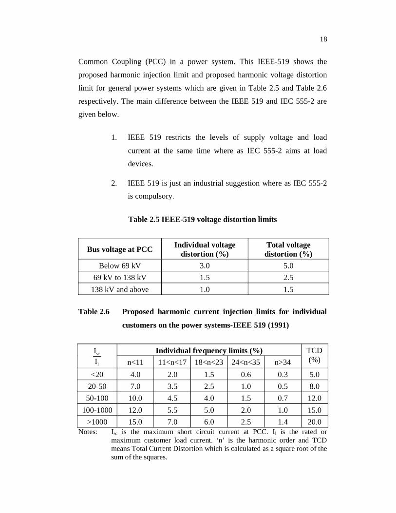
Common Coupling (PCC) in a power system. This IEEE-519 shows the
proposed harmonic injection limit and proposed harmonic voltage distortion
limit for general power systems which are given in Table 2.5 and Table 2.6
respectively. The main difference between the IEEE 519 and IEC 555-2 aregiven below.
1. IEEE 519 restricts the levels of supply voltage and load
current at the same time where as IEC 555-2 aims at loaddevices.
2. IEEE 519 is just an industrial suggestion where as IEC 555-2is compulsory.
Table 2.5 IEEE-519 voltage distortion limits
Bus voltage at PCC Individual voltagedistortion (%)
Total voltagedistortion (%)
Below 69 kV 3.0 5.069 kV to 138 kV 1.5 2.5
138 kV and above 1.0 1.5
Table 2.6 Proposed harmonic current injection limits for individual
customers on the power systems-IEEE 519 (1991)
Individual frequency limits (%)sc
l
II n<11 11<n<17 18<n<23 24<n<35 n>34
TCD(%)
<20 4.0 2.0 1.5 0.6 0.3 5.020-50 7.0 3.5 2.5 1.0 0.5 8.0
50-100 10.0 4.5 4.0 1.5 0.7 12.0100-1000 12.0 5.5 5.0 2.0 1.0 15.0
>1000 15.0 7.0 6.0 2.5 1.4 20.0Notes: Isc is the maximum short circuit current at PCC. Il is the rated or
maximum customer load current. ‘n’ is the harmonic order and TCDmeans Total Current Distortion which is calculated as a square root of thesum of the squares.
19
2.4 HARMONIC ELIMINATION SCHEMES
Arun Arota et al (1998), Das (2004), Key and Lai (1998) have
widely suggested few methods to mitigate the harmonics. Mohamed et al
(2007), Tihamer Adam et al (2002), Yaow-Ming (2003), Zobaa (2004), and
Zacharia et al (2007) have discussed the application of LC filters to control
harmonic component in the power electronic devices. The usage of active
power filter to mitigate the harmonics was explained by Bhim Singh et al
(1998), Bor-Ren Lin et al (2002), Domijan and Embriz-Santander (1990),
Mahanty and Kapoor (2008), and Singh et al (1999). The multi-pulse
technique and pulse width modulation has been described in length by Bowes
and Grewal (1999), Joong-Ho Sung et al (1997), and Trzynadlowsk (1996).
One of the important methods used to mitigate harmonics are passive LC
filters that are used to compensate reactive power and control harmonics. The
principle behind this is to mitigate higher order harmonics by bypassing the
higher order harmonic currents using a capacitor as low impedance. The main
limitation of a passive filter is that its performance is easily influenced by
impedance and operation status of the power grid. This also creates parallel
resonance with system impedance results in magnification of harmonic
current, overload and some times break LC filters. The other simple
mitigation method is using single bandwidth filter, but it is used to control
certain order of harmonics. The principle for the single bandwidth filter is to
create a series resonance for particular frequency and will not allow the back
flow of frequency harmonic current to the system.
In order to overcome the limitations of the passive filter
Bhattacharya et al (1998) proposed the other method to mitigate harmonics by
active power filter which extracts the harmonic current components from
compensated load which in turn create compensation current of opposite
polarity. This kind of filter follows the change of harmonic amplitude and

20
frequency. Its performance is not influenced by the system impedance. The
converter part APF is of two types based on the source type. They are voltage
source type and current source type. 90% of the active power filter
equipments are voltage source type. Depending upon the mode of connection
with the load, active power filters are divided into 2 types namely:
1. Series connected APF
2. Parallel connected APF
Most of the APFs are operated under parallel connection mode and
these are used individually, or along with passive LC Filters. The harmonic
mitigation is carried out effectively by creating a unity power factor
converter, which do not create harmonic current and keep the power factor
value nearer to 1. In some cases, high power factor converters are considered
as unity power factor converter.
In high power factor converter, multi pulse technique and PWM
control technique are effectively used to eliminate lower order harmonics, and
to create waveform similar to sine waveforms. Similar output waveforms are
obtained for pure sine wave if higher levels are used. Multi pulse technique is
mainly used in high power range.
2.5 PULSE WIDTH MODULATION
One of the most widely used strategies for controlling the AC
output of power electronic converters is the technique known as pulse width
modulation, which varies the duty cycle of the converter switches at a high
switching frequency to achieve a target of average or low frequency output
voltage or current.

21
Pulse width modulation techniques has been discussed in detail by
Joachim Holtz (1992) and are used to design the width of pulse sequences so
that a fundamental component voltage with specified magnitude and phase
emerges, and harmonics are shifted towards higher frequency bands. PWM
allows the freedom of controlling the harmonic spectra of the converter
voltage or current. Pulse width modulation does not reduce the total distortion
factor of the current or voltage, but filtering becomes easier (also reduces
filter size) due to the fact that the first present harmonics are of higher order.
A PWM waveform consists of a series of positive and negative
pulses of constant amplitude but with variable switching instances. The
typical goal is to generate a train of pulses such that the fundamental
component of the resulting waveform has a specified frequency and
amplitude. According to Sidney and Paul (1988), the converter switches are
turned on and off several times during each half cycle and the output voltage
is controlled by varying the width of the pulses.
PWM technique has been widely used in DC-AC inverter control. It
effectively reduces the power loss and heat dissipated in the output stage
when delivering power to a load. PWM control strategy results in a pulse train
of fixed amplitude and frequency, only the width of pulse is varied in
proportion to a reference voltage. The end result is that the effective voltage at
the load is proportional to the reference voltage. Due to the rectangular shape
of the output signal, little power is wasted in the output stage. In this way,
PWM techniques offer opportunity to build efficient power delivery systems.
PWM approach is applied when the pulse period of a PWM waveform is
much shorter than the time constant of the load.
Elimination of lower order harmonics from the output of voltage
source PWM inverters brings two major benefits, which were explained by
Sun et al (1994).

22
1. If the inverter is used to supply constant frequency AC power
to general AC loads, a filter is usually installed at its output. In
this case, when lower order harmonics are eliminated through
proper modulation of the inverter, only higher order
harmonics appear at the output and need to be attenuated by
the filter. The cut-off frequency of the filter can thus be
increased, leading to the reduction of the filter size, and
increase in system efficiency.
2. When used in an AC drive system, elimination of lower order
harmonics from the inverter output leads to great reduction of
lower order harmonic torques generated by the motors.
Although harmonic torque is the interaction result between
stator and rotor harmonic currents of different order, higher
order harmonic currents have smaller magnitudes due to the
larger impedance, which the motor presents to higher order
harmonic voltages. Their contributions to lower order
harmonic torques are thus less significant. Therefore, lower
order harmonic torques generated by the motor is greatly
reduced. Consequently, lower frequency resonance of the
mechanical system driven by the motor is avoided.
Various PWM techniques have been designed to minimize
harmonics in converters. They are:
1. Carrier based pulse width modulation
2. Space vector modulation pulse width modulation
3. Third harmonic injection pulse width modulation
4. Selective harmonic elimination pulse width modulation

23
2.5.1 Carrier Based Pulse Width Modulation
According to Antonio Cataliotti et al (2007), Carrier Based PWM
(CBPWM) methods compare a reference waveform with a triangular or
saw-tooth carrier at a higher frequency fs (sampling frequency) and decide
whether to turn a switch on or off. Three significantly different PWM
methods for determining the converter switching on time have been proposed
for fixed frequency modulation systems by Azli and Baskar (2004), Holmes
and Lipo (2003), Sidney and Sukhminder (2000) are as follows,
1. Analog or naturally sampled PWM: Switching at the
intersection of a target reference waveform and a high
frequency carrier.
2. Digital or regularly sampled PWM: Switching at the
intersection between a regularly sampled reference waveform
and a high frequency carrier.
3. Direct PWM: Switching so that the integrated area of the
target reference waveform over the carrier interval is the same
as the integrated area of the converter switched output.
Further, if one sample is used per carrier period, the regular method
is symmetric, while in case of two samples it is asymmetric.
The conventional carrier based method was explained by Halasz
et al (1995), Leon and Thomas (1998) to control a voltage source converter by
Sinusoidal PWM (SPWM), for which the reference waveform is a sinusoidal
waveform. In SPWM the pulse width is not constant but varied by changing
the amplitude of the sinusoidal waveform. In this method a triangular
waveform of a particular amplitude and frequency is compared to a sinusoidal
waveform in phase with the input voltage of an AC/DC converter. Lower

24
order harmonics are eliminated using this technique. A three-phase SPWM
controller essentially consists of three separate SPWM controllers with
reference waveforms that are 1200 out of phase. SPWM is used to control a
Voltage Source Converter (VSC) with two, three, or higher number of levels.
Using the same carrier frequency, the larger the number of voltage levels, the
higher the quality of the output waveform. The number of used carrier
waveforms and the number of switches in each leg, depend on the number of
VSC voltage levels. In SPWM, only the value of the reference waveform at
its intersection with the carrier is used to determine voltage pulses. This
method essentially uses an approximation of the reference waveform.
Figure 2.1 show an example of pulse signal generation for sinusoidal pulse
width modulation reconstruction.
Figure 2.1 Pulse signal generation of sinusoidal pulse width modulation

25
The other types of carrier based pulse width modulation are:
Uniform Pulse Width Modulation (UPWM), and Modified Sinusoidal Pulse
Width Modulation (MSPWM). In UPWM switching is symmetrical causing
all pulses to have the same width. In this method a rectangular waveform of
certain frequency is compared to a rectangular waveform in phase with the
supply voltage. A triangular waveform determines the switching frequency,
and its amplitude determines the width of the pulses. Elimination of certain
harmonics depends on the pulse width chosen. In MSPWM the carrier wave is
applied during the first and last 600 intervals per half cycle. A higher
fundamental waveform component is achieved using the MSPWM.
Elimination of harmonics depends on the switching frequency and is limited
by device switching speed, switching loss and device power ratings.
2.5.2 Space Vector Modulation Pulse Width Modulation
The direct digital technique or the space vector modulation
technique was proposed by Pfaff et al in 1984. This scheme was further
developed by Vander et al in the year 1988 and explained in detail by
Narayanan and Ranganathan (2009), Sidney and Sukhminder (2000), Thomas
and Donald (2005).
Space Vector Modulation (SVM) is one kind of pulse width
modulation strategy, which is quite different from CBPWM methods.
CBPWM methods are based on comparison of a reference waveform with a
high frequency carrier, whereas in the SVM strategy switching instants and
duration of each switching state are calculated from simple equations.
Moreover, there is only one reference vector, in contrast to the three
individual reference waveforms for three phases of the system. It offers more
flexibility as well as a maximum modulation index, M of 1.15.

26
In conventional pulse width modulation strategies, each leg of the
VSC is controlled independently. That is, SPWM uses one sinusoidal
waveform for controlling each of the three legs of the converter. Likewise,
placement of the switching pulses for each leg of a converter under SHE
control is determined separately. In contrast, space vector modulation is
intrinsically designed for three-phase converters. It combines the three
reference waveforms used in CBPWM methods into one single vector, called
the reference space vector. In SVM, instead of modulating waveforms, a
modulating reference vector is employed.
2.5.3 Third Harmonic Injection Pulse Width Modulation
Many other techniques were developed for harmonic elimination in
order to suppress the lower ordered harmonics. The Third Harmonic Injection
PWM (THIPWM) technique was described by Ali (2007), (2008), Boglietti
et al (1995), Kaili Xu et al (2007), and Lawrance et al (1996). According to
them, adding a measure of third harmonic to the output of each phase of a
three-phase inverter, it is possible to obtain a line-to-line output voltage that is
15 percent greater than that obtainable when pure sinusoidal modulation is
employed. The line-to-line voltage is undistorted. This method permits the
inverter to deliver an output voltage approximately equal to the voltage of the
AC supply to the inverter. This method is still being used in dedicated
applications, which describes a technique of injecting third harmonic zero
sequence current components in the phase currents, which greatly improves
the machine torque density. Among all the PWM techniques only a few PWM
strategies have been accepted and used mainly due to the simplicity of
implementation.

27
2.5.4 Selective Harmonic Elimination Pulse Width Modulation
Selective harmonic elimination PWM technique was introduced by
Husmukh and Richard in 1973. The idea of this method is the basic square
wave output is “chopped” a number of times. The chopping time is related to
a set of switching angles of inverter switches, which are obtained by proper
off-line calculations. By appropriate distribution of the switching angles to
turn the inverter bridge switches on and off, the output waveform of the
inverter is controlled and reaches the goal of eliminating lower order
harmonics.
In contrast to carrier based PWM methods, in which switching
instants are determined by direct comparison of reference and carrier
waveforms, in selective harmonic elimination method the exact moments of
switching instants are calculated according to the desired fundamental
component and the harmonic components to be eliminated. Because of
complexity of equations to be solved to find switching instants, the number of
switching angles is normally kept low to make the calculations simple. This
also has the advantage of lowering the converter switching losses and
switching instants are found by offline calculations.
According to Hasmukh and Richard (1974), Chiasson (2004) and
Sirisukprasert et al (2002), the selective harmonic elimination PWM
technique is one of the optimal PWM techniques. It effectively reduces the
harmonics content of inverter output waveform and generate higher quality
spectrum through elimination of specific lower order harmonics. Therefore, it
has been applied in power electronic controllers extensively and many related
techniques have been proposed in recent year. The basic idea is to set up the
notches at the specially designated sites of PWM waveform and the inverter
alters directions many times per half cycle to control the inverter’s output
waveform appropriately.

28
2.6 SHE-PWM WAVEFORM SYNTHESIS
Selective harmonic elimination is used to control both two-level
and higher level voltage source converters. In two-level SHE, for each half
period both +Vdc and Vdc voltage pulses are used, which is called as bipolar
SHE, while in three-level, for each half cycle only one of +Vdc or Vdc is
used, and is known as unipolar SHE. The output waveform of a SHE
modulated VSC is normally constructed in a way that it possesses Quarter
Wave Symmetry (QWS). The output waveform of one phase is expressed in
Fourier series expansion and it is given in equation (2.1).
0 0 01
( ) cos(2 ) sin(2 )n nn
v t a a f nt b f nt (2.1)
where, 0f is the fundamental frequency and ‘n’ is the order of harmonic.
a0, an and bn are the Fourier coefficients and is obtained from ( )v t ,
02 f
Then the expression is written as equation (2.2),
01
( ) cos( ) sin( )n nn
v t a a n t b n t (2.2)
The coefficients a0, an and bn are found from the canonical form
and expressed as equations (2.3)-(2.5).
2
0 dc0
1 V2
a d t (2.3)
2
dc0
1 V cos( )na n t d t (2.4)
and2
dc0
1 V sin( )nb n t d t (2.5)
29
The equation (2.2) is written as equation (2.6).
01
( ) sin( )n nn
v t a c n t (2.6)
where, sinn n na c
cosn n nb c
2 2n n nc a b
1tan where 0nn n
n
a bb
1 0tan 180 where 0nn n
n
a bb
2.6.1 Periodicity
Periodicity of waveforms ensures that they have a discretespectrum. This is guaranteed if the sampling frequency fs is an integer
multiple of fundamental frequency f0 of the reference waveform. Therefore,
the switching pattern of the inverter remains identical in all periods as suchand constructed voltages are also periodic. In order to keep harmonics
minimal, to improve harmonic indices, and to meet the power system
requirements, in addition to periodicity (or synchronization), it is desired thatsynthesized waveforms possess three-Phase Symmetry (3PS), Half Wave
Symmetry (HWS), and quarter wave symmetry.
2.6.2 Three Phase Symmetry
For balanced operation of the load, it is required that the converter
output waveforms possess three-phase symmetry and all harmonics are
balanced. In the particular case of triplen harmonics in a three-phase system,
this leads to their elimination from the line voltages. The necessary and
sufficient condition for 3PS of three-phase voltages is that they are displaced

30
by 1200. For positive sequence, the phase voltages are displaced by 1200 andthey are written in equation (2.7).
23
23
23
a c
b a
c b
v t v t
v t v t
v t v t
(2.7)
2.6.3 Odd Symmetry
If the voltage function ( )v t is periodic function and also contains
symmetries, it satisfies the following periodicity property equation (2.8).
( )v t = ( )v t (2.8)
For periodic functions with odd symmetry, the Fourier coefficientsare given in equation (2.9).
a0 =0
an =0 for all n. (2.9)
2
dc0
4 V sin( ) ( )nb n t d t
A periodic function possessing odd symmetry is written in terms of
an infinite series of only sine functions.
2.6.4 Half Wave Symmetry
While 3PS is targeted at eliminating triplen harmonics, half wave
symmetry eliminates even harmonics. Absence of even harmonics is
particularly important or otherwise they lead to resonance in power networks.

31
Moreover, the DC component, because of changing the operating point of
electrical apparatus, is harmful. A waveform possesses HWS if its mirror in x-
axis shifted by half of the period is identical to itself. If the function ( )v t is
half wave symmetry function and then it satisfies the half wave symmetry
property equation (2.10).
( ) ( )v t v t (2.10)
For periodic function with half wave symmetry, the Fourier
coefficients are given in equation (2.11).
a0=0
an=0 for even n.
2
dc0
4 V cos( ) ( )na n t d t for odd n. (2.11)
bn=0 for even n.
2
dc0
4 V sin( ) ( )nb n t d t for odd n.
A periodic function possessing half wave symmetry has an average
value of zero and its even harmonic components are zero.
2.6.5 Quarter Wave Symmetry
Quarter wave symmetry, which is a subset of HWS, guarantees not
only the even harmonics are zeros, but all harmonics are either in phase or
anti-phase with the fundamental component. Since there are only two phase
angles (00 and 1800) involved for a waveform with such symmetry,
elimination of harmonics by injection requires less effort. This is a desired
feature, although a restrictive one. QWS is obtained if the waveform has

32
symmetry around the midpoints of positive and negative half cycles. This
means that the waveform repeats the same pattern every quarter cycle. Such a
waveform is expressed in equation (2.12).
( ); 02
( );2( )
3( );2
3( ); 22
v t t
v t tv t
v t t
v t t
(2.12)
If the function ( )v t is half wave symmetry and periodic function,
then it is called as odd quarter wave symmetry. For periodic function with odd
quarter wave symmetry, the Fourier coefficients are given by equation (2.13).
a0=0
an=0 for all n.
bn=0 for even n. (2.13)
2
dc0
4 V sin( ) ( )nb n t d t for odd n.
A periodic function possessing odd quarter wave symmetry has
zero average value. The reason is due to the fact that the function is odd. Also,
odd symmetry results in all of the cosine harmonics being zero. Because of
the half wave symmetry of the waveform, all an and even-numbered bn
coefficients are zero. The nth harmonic is eliminated if the respective bn
coefficient is set equal to zero. Also, for a three phase system, triplen
harmonics in the phase voltage are cancelled out in the line voltage and hence,
are not important. Therefore, the lower order harmonics to be removed are
odd, non-triplen components starting as 5, 7, 11, 13, 17…. Selective harmonic

33
elimination pulse width modulation techniques have been mainly developed
for two level (Bipolar) and three-level (Unipolar) converter schemes and
Fourier series expansion of waveforms are explained below.
2.7 UNIPOLAR SELECTIVE HARMONIC ELIMINATION
In unipolar SHE-PWM, the output voltage can be +Vdc, -Vdc or 0.
Figure 2.2 illustrates a unipolar SHE-PWM switching scheme using three
switching angles. Unipolar SHE-PWM uses predetermined switching angles
to produce an output consisting of multiple pulses of varying widths was
discussed in detail by Prasad et al (1990). The number of pulses per
fundamental cycle is equal to twice the number of switching angles used.
Figure 2.2 Unipolar PWM switching scheme
The mathematical models of unipolar programmed PWM scheme
includes single phase application and three phase application were discussed
-----
1
-----
2
---
3
-----
- 3
-------
-----
-----
------------
------------
-------
- 2- 1 + 1
+ 2+ 3 2 - 3
2 - 2 2 - 1

34
by Bouhali et al (2005), Jason et al (2005), Jian Sun and Horst Grotstollen
(1992), Sundareswaran and Mullangi (2002), Vassilios et al (2008). The SHE-
PWM output waveform of three phase application is mathematically obtainedby Fourier series.
1( ) sin( )n
nv t b n t
2
dc0
4 V sin( ) ( )nb n t d t for odd n.
an=0 for all.
The expression for Fourier coefficients of a waveform with Nswitching angles per cycle is given in equation (2.14).
an=0
1dc
1
4V ( 1) cos( )N
in i
ib n
n (2.14)
The equation (2.15) gives the non-zero bn coefficients for an odd n.
dc1 2 3
4V cos cos cos .....nb n n nn
(2.15)
Fourier series expansion of the waveform is given in equation (2.16)and its summarized form is given in equation (2.17).
dc1 2 3
1 2 3
1 2 3
4V( ) cos cos cos ..... sin
sin 3cos3 cos3 cos3 .....3
sin 5cos5 cos5 cos5 .... ....5
v t t
t
t
(2.16)

35
1dc
1,3,.. 1
4V sin( ) 1 cosN
ii
i i
n tv t nn
(2.17)
where, Vdc is the available DC bus voltage and 1 2 ....2N
When there are three switching in each quarter cycle as depicted in
Figure 2.2, three unknowns of 1, 2, and 3 lead to three equations. Again,
one of these equations is used to satisfy the condition on the magnitude of the
fundamental component, and the remaining two equations are used to
eliminate two lowest harmonics (5 and 7). The final set of non-linear
equations for three switching angles is given in the equation (2.18).
dc1 2 3 1
1 2 3
1 2 3
4V cos cos cos
cos5 cos5 cos5 0
cos 7 cos 7 cos7 0
v
(2.18)
Because of the three phase balanced circuit characteristics, the
harmonics whose order is an integer multiple of three, will be cancelled
automatically. The mathematical models of single phase application and three
phase application are the same except that triplen harmonics must also be
eliminated in single phase application.
Unipolar SHE-PWM shares many of the advantages of bipolar
SHE-PWM. Unipolar SHE-PWM is still used with low modulation indices as
well. Like bipolar SHE-PWM, one disadvantage of unipolar SHE-PWM lies
in harmonic distortion. For low modulation indices, unipolar SHE-PWM
leads to an output with higher total harmonic distortion. However, unipolar
SHE-PWM tends to produce a lower THD than bipolar SHE-PWM. It
provides a more natural approximation to a sinusoidal waveform. Unipolar
SHE-PWM also tends to produce less EMI than bipolar SHE-PWM. Bipolar
36
SHE-PWM produces voltage changes equal to 2Vdc. However, unipolar SHE-
PWM produces voltage changes equal to Vdc. Furthermore, unipolar SHE-
PWM increases the effective switching frequency by a smaller factor than
bipolar SHE-PWM.
2.8 BIPOLAR SELECTIVE HARMONIC ELIMINATION
Bipolar SHE-PWM is another switching scheme, which involves
harmonic elimination and was described in detail by Jose et al (2001),
Guzman et al (2004), Maswood and Wei (2005), Salam et al (2003). One
switching scheme involving harmonic elimination that has been widely used
for many years is bipolar SHE-PWM. In bipolar SHE-PWM, the line to neural
output voltage is either +Vdc or –Vdc. The mathematical models of bipolar
programmed PWM scheme includes single phase applications (SLN1: quarter
wave symmetric PWM, switching angle spread 00 to 900 and SLN2: same as
SLN1 with the phase shift, to suppress the first significant harmonic) and
three phase applications (TLN1: quarter wave symmetric PWM, switching
angle spread 00 to 900 and TLN2: quarter wave symmetric PWM, switching
angle spread 00 to 600). Figure 2.3 illustrates the bipolar SHE-PWM switching
scheme using three switching angles for TLN2. Though many different type
of quarter wave symmetric SHE-PWM methods are available for three phase
Voltage Source Inverter (VSI), this thesis deals with TLN1 type of SHE-
PWM technique. The main reason for choosing this type of SHE-PWM is
that, the TLN1 SHE-PWM results in lower harmonic losses and therefore
contributes to lower harmonic heating and consequently lowers derating of
the AC motor drive.
TLN1 waveform has quarter wave symmetry with switching angle
spread 00 to 900, TLN1 waveform is considered for the calculation. The
Fourier series expression for single phase output waveform is expressed in
equation (2.2).

37
Figure 2.3 Bipolar PWM switching scheme
The output waveform of a SHE modulated voltage source converter
is normally constructed in a way that it possesses quarter wave symmetry.
The SHE-PWM output waveform of three phase application which has QWS
is mathematically obtained by Fourier series for TLN1 is given in
equation (2.19).
1( ) sin( )n
nv t b n t
an=0 for all n. (2.19)
2
dc0
4 V sin( ) ( )nb n t d t for odd n.
The expression for Fourier coefficients of a waveform with N
switching angles per cycle is given in equation (2.20).
-----
1
-----
2
---
3
------ 3
-------
-----
-----
------------
------------
-------
- 2- 1 + 1
+ 2+ 3 2 - 3
2 - 2 2 - 1

38
an=0 for all n.
1
4 1 2 ( 1) cos( )N
in i
ib n
n (2.20)
Non-zero bn coefficients are calculated from the equation (2.21).
dc1 2 3
4V 1 2cos 2cos 2cos .....nb n n nn
(2.21)
Fourier series expansions of a waveform with N switching per
quarter cycle are given in equation (2.22) and summarised form is given in
equation (2.23).
dc1 2 3
1 2 3
1 2 3
4V( ) 1 2cos 2cos 2cos ..... sin
sin 31 2cos3 2cos3 2cos3 .....3
sin 51 2cos5 2cos5 2cos5 ..... ....5
v t t
t
t
(2.22)
dc
1,3,.. 1
4V sin( ) 1 2 1 cosN
ii
i i
n tv t nn
(2.23)
where, Vdc is the available DC bus voltage and 1 2 ....2N .
When there are three switching in each quarter cycle, three
unknowns of 1, 2, and 3 lead to three equations. Figure 2.3 shows the
output waveform of a two-level SHE controlled VSC with three switching
angles. One equation is used to satisfy the condition of the magnitude of the
fundamental component, and the remaining two equations are used to
eliminate the 5th and 7th harmonic components. This is shown in the following
equation (2.24).

39
dc11 2 3
1 2 3
1 2 3
4V 1 2cos 2cos 2cos
1 2cos5 2cos5 2cos5 0
1 2 cos7 2 cos7 2cos 7 0
v
(2.24)
The most important advantage of bipolar SHE-PWM is that the
control is not as complicated as in other switching schemes. One of the main
disadvantages of using bipolar SHE-PWM concerns its applicability when
low modulation indices are used. When low modulation indices are used, one
may not be able to use the fundamental switching scheme to perform the
desired harmonic elimination process. Both methods are designed based on
the frequency domain, in contrast to space vector PWM and bipolar
modulation which are based on the time domain. So, these two methods have
greatly reduces harmonic content and are highly recommended from the
medium to the high modulation region. The three-level inverter usually uses
high voltages and is made using Gate Turn Off (GTO) switches which require
a low switching frequency. This fact strongly supports the need to use an
efficient strategy from the medium to the high modulation region.
Some of the methods proposed in the literature for PWM waveform
design are: modulation function techniques, space vector techniques, and
feedback methods. These methods suffer from high residual harmonics that
are difficult to control. A method that theoretically offers the highest quality
of the output waveform is the so-called programmed or optimal PWM. A
sizable amount of work has been done on the optimal solution for the
transcendental equations describing the SHE-PWM switching patterns.
40
2.9 SOLUTION METHODOLOGY FOR HARMONIC
ELIMINATION
Many methods are available presently for the optimal solution of
non-linear equations explained by Ali et al (2001), Dariusz et al (2002), Hyo
et al (1995), Jurgen (1992) and these methods are based on mathematical
programming techniques involving gradient search discussed by Maswood
et al (1998) and direct search assuming that, the design variables are
continuous. The main challenge associated with SHE-PWM techniques is to
obtain the analytical solution for the resultant system of non-linear
transcendental equations that contain trigonometric terms which in turn
provide multiple sets of solutions, which was enumerated by Vassilios et al
(2004). Several algorithms have been reported in the technical literature
concerning methods of solving the resultant non-linear transcendental
equations, which describes the SHE-PWM problem. For SHE-PWM, the
switching instants are determined by solving a set of non-linear equations.
Due to non-linear and transcendental characteristics, such equation can only
be solved numerically.
To obtain fast convergence, the initial values must be selected close
to the exact solutions. This is one of the most difficult tasks associated with
programmed PWM techniques. However, it is difficult to derive the solutions
for simultaneous transcendental equations for eliminating selected harmonics
in real time applications. It is interesting to observe that the applied
optimization technique, which finds the solution for higher values of
modulation indices without any failure in convergence.
The problem is formulated around the desired value of the
fundamental component to be generated. This method then seeks to find the
angles that would provide fundamental amplitude and, would result in the
elimination of a number of selected harmonics. The generalized case is to find
41
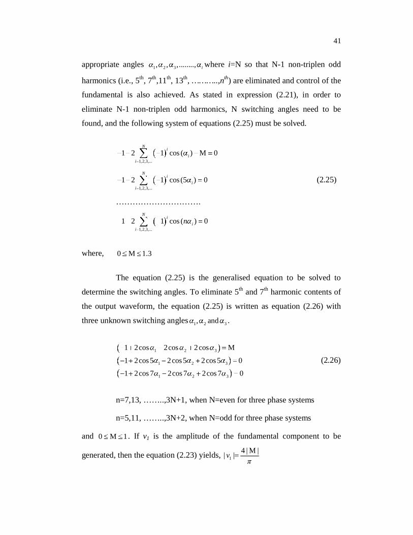
appropriate angles 1 2 3, , ,........, i where i=N so that N-1 non-triplen odd
harmonics (i.e., 5th, 7th,11th, 13th, ………..,nth) are eliminated and control of the
fundamental is also achieved. As stated in expression (2.21), in order to
eliminate N-1 non-triplen odd harmonics, N switching angles need to be
found, and the following system of equations (2.25) must be solved.
1,2,3,...
1 2 1 cos ( ) M 0N
ii
i
1,2,3,...
1 2 1 cos (5 ) 0N
ii
i
(2.25)
………………………….
1,2,3,...
1 2 1 cos ( ) 0N
ii
i
n
where, 0 M 1.3
The equation (2.25) is the generalised equation to be solved to
determine the switching angles. To eliminate 5th and 7th harmonic contents of
the output waveform, the equation (2.25) is written as equation (2.26) with
three unknown switching angles 1 2 3, and .
1 2 3
1 2 3
1 2 3
1 2cos 2cos 2cos M
1 2cos5 2cos5 2cos5 0
1 2cos 7 2cos 7 2cos 7 0
(2.26)
n=7,13, ……..,3N+1, when N=even for three phase systems
n=5,11, ……..,3N+2, when N=odd for three phase systems
and 0 M 1 . If v1 is the amplitude of the fundamental component to be
generated, then the equation (2.23) yields, 14 | M || |v
42
Choosing the switching angles such that a desired fundamental
output is generated and specifically selected harmonics of the fundamental are
suppressed. This is referred as harmonic elimination or programmed harmonic
elimination as the switching angles are selected to eliminate a specific
harmonics. The harmonic elimination problem was formulated as a set of
transcendental equations that must be solved to determine the switching
angles in an electrical cycle for turning the switches on and off in a full bridge
inverter so as to produce a desired fundamental amplitude while eliminating
the specific order of harmonics. These transcendental equations are then
solved using iterative numerical techniques mentioned by Chunhui et al
(2005) to compute the switching angles.
In order to proceed with the optimization/minimization, an
objective function describing a measure of effectiveness for eliminating
selected order of harmonics while maintaining the fundamental at a pre-
specified value must be defined. This is converted to an optimization problem
subject to constraints. The task is to determine the firing instants such that
objective function F ) (2.27) is minimized. Therefore, the output voltage is
regulated ideally over the full range [0, Vdc] by changing the modulation index
M and has no harmonics within that range, to obtain the switching instants.
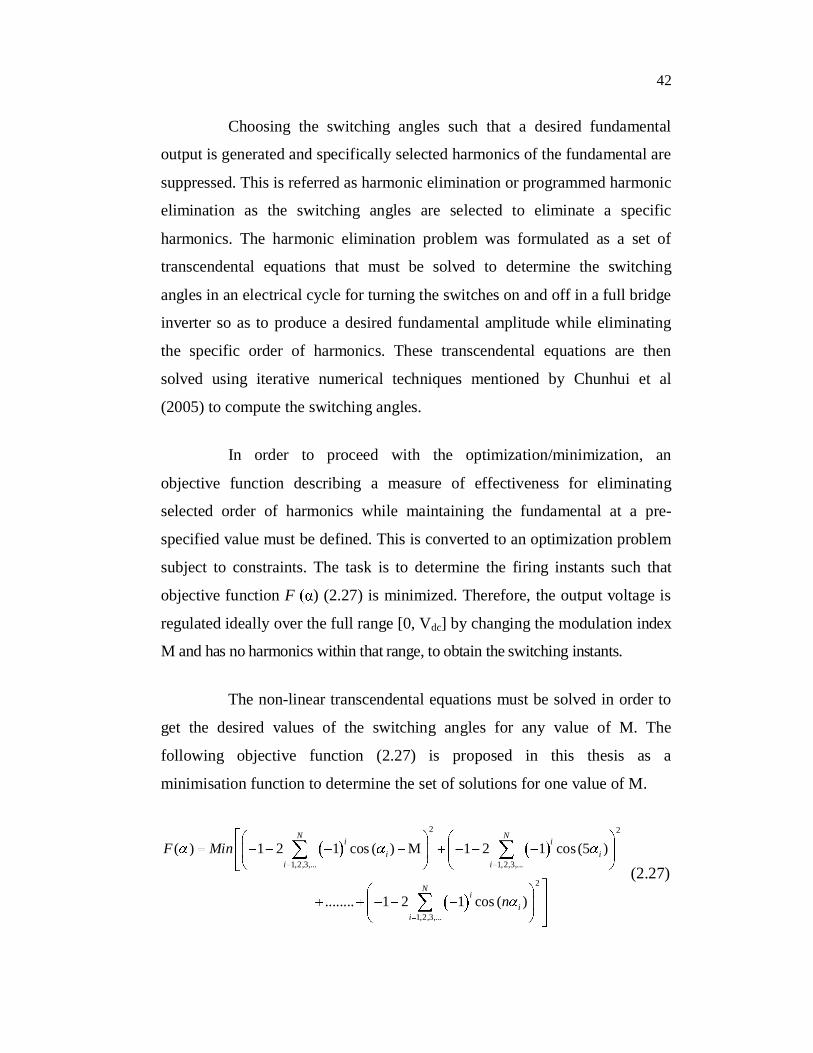
The non-linear transcendental equations must be solved in order to
get the desired values of the switching angles for any value of M. The
following objective function (2.27) is proposed in this thesis as a
minimisation function to determine the set of solutions for one value of M.
2 2
1,2,3,... 1,2,3,...
2
1,2,3,...
( ) 1 2 1 cos ( ) M 1 2 1 cos(5 )
........ 1 2 1 cos ( )
N Ni i
i ii i
Ni
ii
F Min
n
(2.27)
43
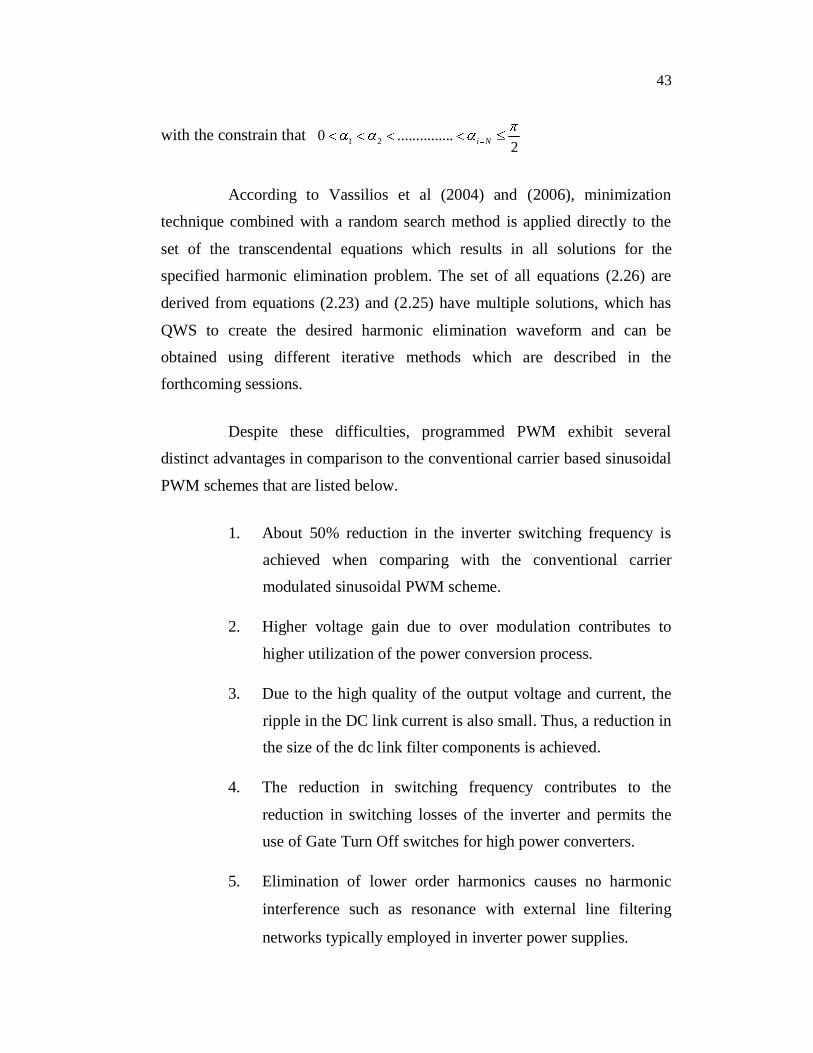
with the constrain that 1 20 ...............2i N
According to Vassilios et al (2004) and (2006), minimizationtechnique combined with a random search method is applied directly to the
set of the transcendental equations which results in all solutions for thespecified harmonic elimination problem. The set of all equations (2.26) are
derived from equations (2.23) and (2.25) have multiple solutions, which has
QWS to create the desired harmonic elimination waveform and can beobtained using different iterative methods which are described in theforthcoming sessions.
Despite these difficulties, programmed PWM exhibit severaldistinct advantages in comparison to the conventional carrier based sinusoidal
PWM schemes that are listed below.
1. About 50% reduction in the inverter switching frequency isachieved when comparing with the conventional carriermodulated sinusoidal PWM scheme.
2. Higher voltage gain due to over modulation contributes to
higher utilization of the power conversion process.
3. Due to the high quality of the output voltage and current, the
ripple in the DC link current is also small. Thus, a reduction inthe size of the dc link filter components is achieved.
4. The reduction in switching frequency contributes to the
reduction in switching losses of the inverter and permits theuse of Gate Turn Off switches for high power converters.
5. Elimination of lower order harmonics causes no harmonic
interference such as resonance with external line filtering
networks typically employed in inverter power supplies.

44
A fundamental issue in the control of a voltage source inverter is to
determine the switching angles, so that the inverter produces the required
fundamental voltage and does not generate specific lower dominant
harmonics. Due to its inherent non-linear nature, the system for harmonic
elimination equations has to be solved numerically and for this propose
iterative technique such as Newton Raphson iterative algorithm is used to
obtain the desired solutions for the angles. The various traditional methods
used to solve the transcendental equations in order to eliminate the lower
order harmonics are listed below.
2.10 NEWTON RAPHSON ITERATIVE METHOD
At this particular phase, an iterative algorithm such as the Newton–
Raphson is used to obtain the desired solutions for the angles. The iterative
method is implemented using a software package such as Mathematica.
Due to its inherent non-linear nature, the system of harmonic
elimination equations (2.25) has to be solved numerically and for this purpose
Newton Raphson iterative Algorithm which was described by Benghanem
and Draou (2005), Sahali and Fellah (2003), Sun and Grotstollen (1994a) is
found to be very effective. For three phase inverter, the system of harmonic
elimination equations is given in equation (2.25). For given M, this algorithm
solves harmonic elimination equations iteratively in the following sequence:
1. Initial guess of a string point (k) for k=0.
2. Formulation of a local linear model using Newton Raphson
method is given by the equation (2.28).( ) ( ) ( )J ( ). ( ) 0k k kf (2.28)
3. Solving of local linear model (2.28) for (k).
4. Updating: ( 1) ( ) ( )k k k ; k=k+1, return to 2

45
Here f( ), the vector represents the left hand sides of harmonic
elimination equations (2.26) and J ) is the Jacobian matrix of f( ). The
Jacobian matrix for the harmonic elimination equations (2.26) is written by
the equation (2.29).
1 2 3
1 2 3
1 2 3
2sin 2sin 2sinJ ( ) 10sin 5 10sin 5 10sin 5
14sin 7 14sin 7 14sin 7
f (2.29)
It is formally proved that the Jacobian matrix J( ) of three-phase
harmonic elimination equation is non-singular, regardless of the waveform
structure and the number of switching angles. The only condition is that the N
switching angles should be distinct from each other and not equal to 0, that
is 1 2 N0 ............2
. This guarantees that the local linear model
(2.28) is solved without any numerical difficulty.
However, providing a suitable initial guess (0) which must be close
enough to the exact solution so as to ensure the convergence of Newton’s
algorithm is not a trivial task and deserves special attention. The traditional
method for solving SHE-PWM problem using Newton Raphson algorithm,
whose main shortcoming is that the results deeply depend on the selection of
initial values.
Commonly, for different numerical algorithms used for solving
SHE-PWM switching pattern, some specific analyses must be taken to preset
the initial values and predict the trend of these values over whole range of
modulation index.
Traditional optimization methods suffer from various drawbacks,
such as prolonged period, tedious computational steps and convergence to
local optima; thus, the more the number of harmonics to be eliminated, the

46
larger the computational complexity and time required. The traditional PWM
method cannot completely eliminate the specified lower order harmonics.
This programmed method is also called as computed PWM method, since
their pulses are computed.
2.11 RESULTANT THEORY
A fundamental issue in the control of a voltage source inverter is to
determine the switching angles so that the inverter produces the required
fundamental voltage and does not generate specific lower dominant
harmonics. The approach demonstrated here is accomplished by transforming
the non-linear transcendental harmonic elimination equations for all possible
switching schemes into a single set of symmetric polynomial equations in the
first step. Then it is shown that a particular switching scheme is simply
characterized by the location of the roots of these polynomial equations. For
each value of M, the complete set of solutions to the equations is found using
the method of resultants from elimination theory was discussed in detail by
John et al (2002), (2003), (2004), (2005), Leon et al (2005) and Zhong et al
(2004), (2004a).
The Fourier series expansion of the output voltage waveform is
given in equation (2.24). The main objective of this method is to determine
the switching angles 1 2 3, and to obtain the desired fundamental voltage
v1(t). To use the resultant theory method, the harmonic elimination
equations (2.26) are first converted to an equivalent polynomial system.
Specifically, one defines 1 1 2 2cos , cos ,x x 3 3cosx and uses the
trigonometric identities.
3 5
3 5 7
cos(5 ) 5cos 20cos 16cos
cos(7 ) 7cos 56cos 112cos 64cos

47
To transform the conditions (2.26) into the equivalent conditions.
1 1 2 3
33 5
51
33 5 7
71
( ) 1 M 2 2 2 0
( ) 1 2 ( 1) (5 20 16 ) 0
( ) 1 2 ( 1) ( 7 56 112 64 ) 0
ii i i
i
ii i i i
i
p x x x x
p x x x x
p x x x x x
(2.30)
where, 1 2 3( , , )x x x x and 1M /(4 / )dcV V . Equation (2.30) is a set of the
polynomial equations with three unknowns 1 2 3, ,x x x . Further, the solutions
must satisfy the condition 3 2 10 1x x x . Such a transformation to
polynomial equations was used by Sahali and Fellah (2003), where the
polynomials were then solved using iterative numerical techniques. In
contrast, it is shown here how the polynomial equations are solved directly for
all solutions.
2.11.1 Elimination using Resultants
In order to explain how one computes the zero sets of polynomial
systems, a brief procedure for solving such systems is given. A systematic
procedure to do this is to apply the elimination theory and use the notion of
resultants. Briefly, one considers 1 2( , )a x x and 1 2( , )b x x as polynomials in 2x
whose coefficients are polynomials in 1x . Then, for example, letting
1 2( , )a x x and 1 2( , )b x x have degrees 3 and 2, respectively in 2x , they are written
as the equation (2.31).
3 21 2 3 1 2 2 1 2 1 1 2 0 1
21 2 2 1 2 1 1 2 0 1
( , ) ( ) ( ) ( ) ( )
( , ) ( ) ( ) ( )
a x x a x x a x x a x x a x
b x x b x x b x x b x (2.31)
The p p Sylvester matrix,

48
where2 21 2 1 2deg ( , ) deg ( , ) 3 2 5x xp a x x b x x , is defined by the
equation (2.32).
0 1 0 1
1 1 0 1 1 1 0 1
, 1 2 1 1 1 2 1 1 1 0 1
3 1 2 1 2 1 1 1
3 1 2 1
( ) 0 ( ) 0 0( ) ( ) ( ) ( ) 0
( ) ( ) ( ) ( ) ( ) ( )( ) ( ) 0 ( ) ( )0 ( ) 0 0 ( )
a b
a x b xa x a x b x b x
S x a x a x b x b x b xa x a x b x b x
a x b x
(2.32)
The resultant polynomial is then defined by the equation (2.33).
The equation (2.33) is the result of solving 1 2( , ) 0a x x and
1 2( , ) 0b x x simultaneously for 1x , that is for eliminating 2x .
1 , 1( ) det ( )a br x S x (2.33)
2.11.2 Solving the Bipolar Equations
The resultant methodology is used to solve all possible switching
angles. That is 3 1 2M ( )x x x is used to eliminate 3x from 5p and 7p in (2.30)
to get the two polynomial equations 5 1 2( , ) 0p x x , 7 1 2( , ) 0p x x with two
unknowns which must be solved simultaneously. This is reduced to one
polynomial given in equation (2.34) with one unknown by computing the
resultant polynomials5 7, 1( )p pr x of the polynomial pair 5 1 2 7 1 2( , ), ( , )p x x p x x .
5 7
2 4 2, 1 1 1( ) 16777216M (1 M 2 ) ( )
bip pr x x r x (2.34)
where 1( )bir x is a polynomial of 9th degree which is described by Chiasson et al
(2004). As the parameter M is incremented in steps of 0.01, the roots of 1( )bir x
are found and used to back solve for 2x and 1x . The set of all three unknowns

49
3 2 1( , , )x x x which satisfies 3 2 10 1x x x are used to calculate the switching
angles for the harmonic elimination equations.
1 1 13 2 1 1 2 3{( , , )} cos , cos , cosx x x (2.35)
The set of all possible solutions to (2.25) for the particular value of
M is given in the equation (2.35). This computation was done for the various
value of M by incrementing the value of M between 0 and 1.
According to John et al (2002), (2004), and Leon et al (2005), the
difficulty of this approach is that when there are several DC sources, the
degrees of the polynomials are quite large, thus making the computational
burden of resultant polynomials quite high. However, the method introduces
another step into the problem through the manipulation of higher order
polynomials whose order increases as the number of harmonics to be
eliminated also increases. Furthermore, it has limited chance to work for a
higher order of harmonics and it is easy to apply only when such numbers are
low.
2.12 CURVE FITTING TECHNIQUE
One of the most popular real world applications of mathematics is
curve fitting. Curve fitting involves examining what might seem like a
random data set and deriving an equation that strongly describes that set.
Functions commonly used for the purpose of curve fitting include exponential
and logarithmic functions, but polynomial functions probably hold the most
important role. Development of equations based on a curve fitting technique
was discussed by Ahmad and Yatim (2001), (2001a), (2002), Salam and Lynn
(2002), Salam et al (2003), Salam (2004), Tan and Bian (1991), that can be
used to calculate the optimal switching angles.

50
The equations (2.26) that need to be solved are transcendental in
nature and incorporate periodic trigonometric terms, which means more than
one set of solutions usually exists. To calculate the optimal PWM switching
angles for the VSI, a Curve Fitting Technique (CFT) is adopted due to the
curvilinear or non-linear feature of the switching angles solutions trajectories.
This method is based on quadratic approximation approach which is derived
from the computed trajectories of angles. The CFT involves accurate
representation of each of these trajectories by the equations in terms of
switching angle and modulation index. The coefficients of these polynomials
are computed by simple minimization technique. MATLAB curve fitting
function, based on polynomial regression is found to be adequate tool to
approximate the trajectories. The algorithm results in quadratic equations
which require only the multiplication process and therefore this technique is
implemented efficiently.
2.13 NELDER-MEAD SIMPLEX ALGORITHM
The minimization problem to find the set of solutions for one value
of M was dealt with using the Nelder–Mead simplex algorithm by Quintana
et al (1989). The Nelder-Mead algorithm technique in combination with a
random search finds all the sets of possible solutions for one value of M, that
is M = 0.1 and then such information is used as initial value to find all
possible sets of solutions for all values of M. Specifically, for the next value
of M, the solutions from the previous value of M are used as an initial point.
According to Nelder and Mead (1965), the algorithm is used to find the first
or initial set of solutions for the given non-linear equations. An iterative
algorithm such as the Newton–Raphson algorithm can be used to obtain the
desired solutions for the angles. This is done to further improve the speed of
the method.
51
2.14 CHEBYSHEV POLYNOMIALS
Chebyshev’s Polynomials are of great importance in many area of
mathematics, particularly approximation theory. The Chebyshev polynomials
have many properties and applications, arising in a variety of continuous
settings. They are a sequence of orthogonal polynomials appearing in
approximation theory, numerical integration and differential equations. The
trigonometric identity of Chebyshev property which was used in this method
is given in the equation (2.36).
ncos(n )=T cos( ) (2.36)
where, Tn is the Chebyshev polynomial of the first kind.
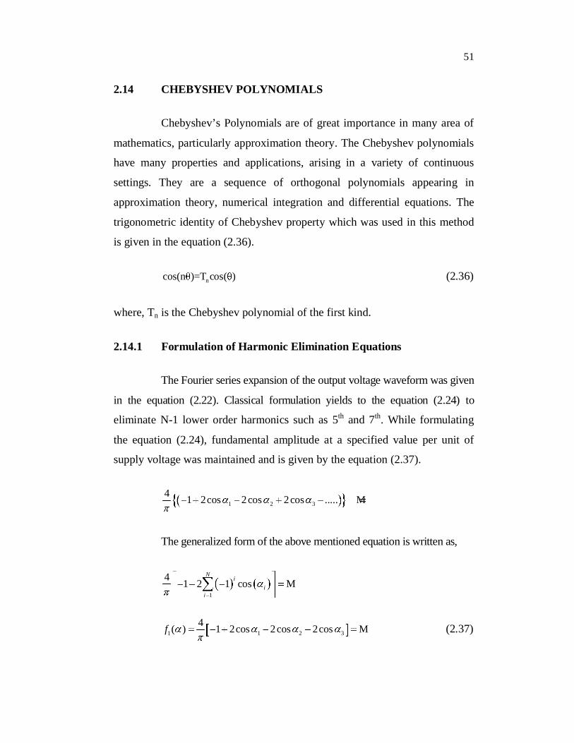
2.14.1 Formulation of Harmonic Elimination Equations
The Fourier series expansion of the output voltage waveform was given
in the equation (2.22). Classical formulation yields to the equation (2.24) to
eliminate N-1 lower order harmonics such as 5th and 7th. While formulating
the equation (2.24), fundamental amplitude at a specified value per unit of
supply voltage was maintained and is given by the equation (2.37).
1 2 34 1 2cos 2cos 2cos ..... M
The generalized form of the above mentioned equation is written as,
1
4 1 2 1 cos MN
ii
i
1 1 2 34( ) 1 2cos 2cos 2cos Mf (2.37)

52
The modulation index, M indicates the fundamental component of
output voltage. Therefore, SHE-PWM comprises of such a degree of freedom
in order to control the amplitude of fundamental component, permits the
elimination of N-1 odd harmonics. Equation (2.37) is rewritten as
equations (2.38) and (2.39).
1( ) M( ) 0n
ff
(2.38)
11
13,5,......,2 1
1 M( ) ( 1) cos 1 02 4
1( ) ( 1) cos 02
Ni
ii
Ni
n ii
n N
f
f n (2.39)
The equations (2.39) is written as equation (2.40)
1 2
( ) ( ) 0
, ,................,n
TN
F f (2.40)
2.14.2 Transformation in to an Algebraic System
The solutions of these sets are tedious, because they yield to a trial
and error process with additional difficulties due to convergence problems.
The Chebyshev polynomials of the first kind can be defined by the
trigonometric theory is given by the equation (2.41).
1
1 2
T ( ) cos (cos )( ) ( ) 0
, ,................,
n
n
TN
x n xF x f x
x x x x
(2.41)
where, 10 cos 1x
x is the solution vector.

53
The roots of the Tn(x) are (2 1)cos2
in
i=1,2,….,n
Using Chebyshev polynomial theory, the problem is alternatively
formulated by transforming the trigonometric equations into algebraic
equations is given by the equation (2.42).
11
13,5,.........2 1
1 M( ) ( 1) T ( ) 1 02 4
1( ) ( 1) T ( ) 02
Ni
i ii
Ni
n n ii
n N
f x x
f x x (2.42)
The most useful process for solving systems of non-linear equations
shown above (2.41) is based on Newton method. The Newton-Raphson
method tries to solve the non-linear set of equations (2.41) iteratively and
solution vector is updated using the equation (2.44) until the stopping criteria
are met. These linear system of equation (2.42) are satisfactorily solved by
means of an iterative process equations (2.43) and (2.44) by the application of
Newton-Raphson or Gauss reduction methods.
( ) ( ) ( )J( ) 0i i ix x Fx (2.43)
( 1) ( ) ( )i i ix x x (2.44)
where,
1 1
1
1
...........
......................J ( )
.......................
..........
n
n n
n
dF dFdx dx
x
dF dFdx dx
is the Jacobian matrix of F(x).
( )ix is the derivative of the solution vector.

54
The fundamental amplitude of the output voltage was obtained by
initializing the value of modulation index, M=0 and the solution vector as
initial vector x(0). The successive values of the switching angles have been
calculated according to an increment M and using the solution vector x as an
initial value for the next. By keeping M=0.01, the calculation is repeated for
the range of modulation index 0 M 1.0 .
The main advantages of Chebyshev function method are as follows:
1) The use of algebraic variables avoids the restrictive margin
(1,-1) of the trigonometric ones and provides an excellent
convergence ratio.
2) It improves the processing time due to minimization of the
trigonometric functions application.
2.15 WALSH HARMONIC ELIMINATION METHOD
The Walsh function harmonic elimination method was first
introduced by Asumadu and Hoft (1989). This function forms an ordered set
of rectangular waveforms taking only two amplitude values +1 and -1, over
one normalized frequency period. The walsh function forms a complete
orthogonal set; hence walsh functions can be used to represent signals in the
same way as the Fourier series. By using the walsh function analytic
technique, the harmonic amplitude is expressed directly as a function of
switching angles was described by Chunfang et al (2005), Liang and Hoft
(1993), Nazarzadeh et al (1997), Swift and Kamberis (1993), Tsorng-Juu et al
(1997). Then, linear algebraic equations are solved to obtain the switching
angles resulting in elimination of unwanted harmonics. The global solution is
found by searching all possible switching patterns, since the local solutions
are obtained only under an appropriate initial condition. This method is not

55
very efficient when a large number of lower order harmonics need to be
eliminated.
2.16 HOMOTOPY BASED COMPUTATION
A systematic homotopy based computation method is used to solve
the SHE problem, which has been proposed by Kato (1999). This method
finds multiple solutions for a specific N switching angles reducing
N-1harmonic content from the output of the circuit by varying a fundamental
component value as the homotopy parameter. However, the method is long
and cumbersome and the method does not make any contribution towards the
set of solutions from the multiple available ones is optimum against overall
harmonic performance and presents no experimental results to confirm the
analysis.
2.17 EIGEN SOLVE ALGORITHM
Though computing the roots for a non-linear polynomial, which has
received much discussion in the literature so far, it is still a tedious problem
for numerical computation. Recently, the eigen solve algorithm is proposed
by Fortune (2002), which computes the zeros of polynomials. The method is
based on iterative conditioning technique. That is, given an unconditioned
instance, the problem is first solved by a standard algorithm and the result is
then used to compute a new instance which is better conditioned or at some
times has the same solution as the original one. The iteration is repeated until
a well conditioned instance (which can be easily solved) is obtained. It is
shown by Han et al (2004) that the eigen solve algorithm can effectively
compute all zeros for highly ill-conditioned polynomial, and is faster than the
best alternative in an order of magnitude. An eigen solve algorithm is
introduced to non-linear equations and it is especially good for solving the
highly ill-conditioned polynomial.

56
2.18 NEURAL NETWORK METHOD
Application of neural networks to the optimal control of three phase
voltage controlled inverters was descried by Andrzej and stanislaw (1992),
Mohaddes et al (1997). Pre-calculated switching angles for the elimination of
lower order harmonics of the output voltage are used to train a software
emulated network. The trained network generates approximate switching
angles in response to the required value of the modulation index applied to its
output. A neural network to be used for the generation of optimal switching
angles have single input accepting desired values of the modulation index and
time of the first quarter switching angles. A hidden layer is necessary to
provide the required number of degrees of freedom for accurate mapping.
2.19 EQUAL AREA ALGORITHM METHOD
The pulse width in each sampling interval is determined by making
the area of the inverter output equal to the area of sinusoidal reference
voltage, which is shown in Figure 2.4.
Figure 2.4 Equal area PWM algorithm
57
The pulse width in each sampling interval is given by the
equation (2.45).
m1
dc
V( ) cos cosV i idt i t t
w(2.45)
The switching angles in a sampling interval are given in
equation (2.46).
1
2
T( 0.5) ( ) / 2T( 0.5) ( ) / 2, where, 0,1, 2.....
i
i
i dt ii dt i i
(2.46)
where,
1i is the (i+1)th switching angle
ti is the ith sampling time
dt(i) is the ith sampling pulse width
Vdc is the input DC voltage
Vm is the maximum sinusoidal voltage
w is the sampling frequency
T is the sampling period
The switching angles obtained by equal area algorithm described by
Chen and Liang (1997), Jyh-Wei (2005) are the starting values for numerical
analysis. This method is also one of the methods used to find the starting
solution values for first set of solution values or starting values of the non-
linear transcendental equations.
The global solution is found by searching all possible switching
patterns since the local solutions are obtained only under an appropriate initial
condition. These traditional methods are not very efficient when a large
number of lower order harmonics need to be eliminated.

58
2.20 NON-TRADITIONAL METHODS
The main advantages of the non-traditional optimization technique,
when compared to traditional methods are the following. No preliminary
calculations are necessary to find the solutions of non-linear transcendental
equations. In fact, these values are not necessary for the division of the entire
solution space into small regions to ensure convexity.
Many non-traditional techniques have become admired in
engineering optimization problem and recently, stochastic approach has
achieved increasing popularity among researchers. The efficiency of these
iterative solution methods depends mostly on the modelling. A fine tuning of
parameters will never balance a bad choice of the neighbourhood structure or
of the objective function. An effective modelling should lead to robust
techniques that are not too sensitive for different parameter settings. There
have been many approaches to this problem reported in the technical literature
including: Genetic algorithm described by Al-Othman et al (2007), Burak
et al (2005), Han et al (2004a), Hasanzadeh et al (2003), John et al (2004),
Maswood et al (2001), Mohamed et al (2006), (2008), Shen and Ali (2000),
Shi and Hui Li (2005), Sundareswaran and Mullangi (2002), Yaow-Ming
(2003), Ant colony search algorithm applied by Kinattingal et al (2007),
Simulated Annealing explained by Leopoldo et al (2007) and particle swarm
optimization mentioned by Said et al (2008). The bipolar waveform has been
treated in detail by Hasanzadeh et al (2003) where a minimization technique
is employed along with a biased optimization search method to get the
multiple sets of solution.
The voltage source inverter with non-traditional methods
optimization solution significantly enhances the handling capacity of power
electronics equipments using currently available switching devices without
bulky transformer connections and problematic series connections. The use of

59
optimization techniques including genetic algorithm has been shown to
overcome all known obstacles of the previous approaches, which was
explained by Dahidah and Agelidis (2005).
There are many advantages that make genetic algorithm attractive
was mentioned by Frenzel (1993). Genetic algorithm does not require the use
of derivatives. They offer a parallel searching of the solution space rather than
the point-by-point searching in a small region. Since the location of the
optimal solution is unknown before the search, it is very likely that the point-
by-point search needs to search through the entire solution space in order to
find the optimal solution, not to mention the traps of the local optima. Hence,
genetic algorithm can find a near optimal solution for a complex problem very
quickly and efficiently.
2.21 CONCLUSION
In this chapter, various pulse width modulation techniques for
inverter/converter circuits have been presented. Among various methods,
SHE-PWM has its own advantages in modern power electronics applications.
Selective harmonic elimination PWM technique, is a kind of popular control
signal generation technique, is widely used in UPS, reactive power
compensators and power filters. It has a clear physical model and is easy to
realize. However, its complex multi root transcendental equations provide
difficulties for root finding. Consideration of special characteristics of SHE-
PWM allowed for obtaining results which offer ideas for optimization of
output spectrum by employing advanced algorithms and analog circuits.
Many methods are there to find optimum solution for non-linear
transcendental equations.
Due to the special characteristics of SHE-PWM output spectrum,
some minimization techniques have been used to solve the non-linear

60
transcendental equations. The details of solving the non-linear equations using
the traditional algorithms are explained in this chapter. These methods have
their own shortcomings to find the initial values for the solution of the
equations. In the proceeding chapters, the usage of non-traditional methods to
solve the transcendental equations is given in detail by overcoming the
disadvantages of traditional minimization techniques. By optimizing the
switching angles distribution, the harmonic content can be flexibly
redistributed and high quality output waveforms are obtained.
![Statistical methods for body mass index: a selective …arXiv:1412.3653v1 [stat.AP] 11 Dec 2014 Statistical methods for body mass index: a selective review of the literature Keming](https://img.pdfslide.us/doc/110x75/5e59b7fc2f7b50503c646c1a/statistical-methods-for-body-mass-index-a-selective-arxiv14123653v1-statap.jpg)