Chapter 2latcha/me486/BN10/Chap02_10e.pdf · Shigley’s MED, 10 th edition Chapter 2 Solutions, Page 1/22 Chapter 2 2-1 From Tables A-20, A-21, ... 9 100 0.196 3 0.012 15 46 357.6

Shigley’s MED, 10th edition Chapter 2 Solutions, Page 1/22

Chapter 2 2-1 From Tables A-20, A-21, A-22, and A-24c, (a) UNS G10200 HR: Sut = 380 (55) MPa (kpsi), Syt = 210 (30) MPa (kpsi) Ans. (b) SAE 1050 CD: Sut = 690 (100) MPa (kpsi), Syt = 580 (84) MPa (kpsi) Ans. (c) AISI 1141 Q&T at 540°C (1000°F): Sut = 896 (130) MPa (kpsi), Syt = 765 (111) MPa (kpsi) Ans. (d) 2024-T4: Sut = 446 (64.8) MPa (kpsi), Syt = 296 (43.0) MPa (kpsi) Ans. (e) Ti-6Al-4V annealed: Sut = 900 (130) MPa (kpsi), Syt = 830 (120) MPa (kpsi) Ans. ______________________________________________________________________________ 2-2 (a) Maximize yield strength: Q&T at 425°C (800°F) Ans. (b) Maximize elongation: Q&T at 650°C (1200°F) Ans. ______________________________________________________________________________ 2-3 Conversion of kN/m3 to kg/ m3 multiply by 1(103) / 9.81 = 102 AISI 1018 CD steel: Tables A-20 and A-5

( )( )

3370 1047.4 kN m/kg .

76.5 102yS

Ansρ

= = ⋅

2011-T6 aluminum: Tables A-22 and A-5

( )( )

3169 1062.3 kN m/kg .

26.6 102yS

Ansρ

= = ⋅

Ti-6Al-4V titanium: Tables A-24c and A-5

( )( )

3830 10187 kN m/kg .

43.4 102yS

Ansρ

= = ⋅

ASTM No. 40 cast iron: Tables A-24a and A-5.Does not have a yield strength. Using the ultimate strength in tension

( )( )

( )

342.5 6.89 1040.7 kN m/kg

70.6 102utS

Ansρ

= = ⋅

______________________________________________________________________________ 2-4 AISI 1018 CD steel: Table A-5

( ) ( )

6

630.0 10

106 10 in .0.282

EAns

γ= =

2011-T6 aluminum: Table A-5

( ) ( )

6

610.4 10

106 10 in .0.098

EAns

γ= =


Ti-6Al-6V titanium: Table A-5

( ) ( )

6

616.5 10

103 10 in .0.160

EAns

γ= =

No. 40 cast iron: Table A-5

( ) ( )

6

614.5 10

55.8 10 in .0.260

EAns

γ= =

______________________________________________________________________________ 2-5

22 (1 )

2

E GG v E v

G

−+ = ⇒ =

Using values for E and G from Table A-5,

Steel: ( )

( )30.0 2 11.5

0.304 .2 11.5

v Ans−

= =

The percent difference from the value in Table A-5 is

0.304 0.292

0.0411 4.11 percent .0.292

Ans− = =

Aluminum: ( )

( )10.4 2 3.90

0.333 .2 3.90

v Ans−

= =

The percent difference from the value in Table A-5 is 0 percent Ans.

Beryllium copper: ( )

( )18.0 2 7.0

0.286 .2 7.0

v Ans−

= =


0.286 0.285

0.00351 0.351 percent .0.285

Ans− = =

Gray cast iron: ( )

( )14.5 2 6.0

0.208 .2 6.0

v Ans−

= =


0.208 0.211

0.0142 1.42 percent .0.211

Ans− = − = −

______________________________________________________________________________ 2-6 (a) A0 = π (0.503)2/4 = 0.1987 in2, σ = Pi / A0


For data in elastic range, ∫ = ∆ l / l0 = ∆ l / 2

For data in plastic range, 0 0

0 0 0

1 1l l Al l

l l l A

−∆= = = − = −ò

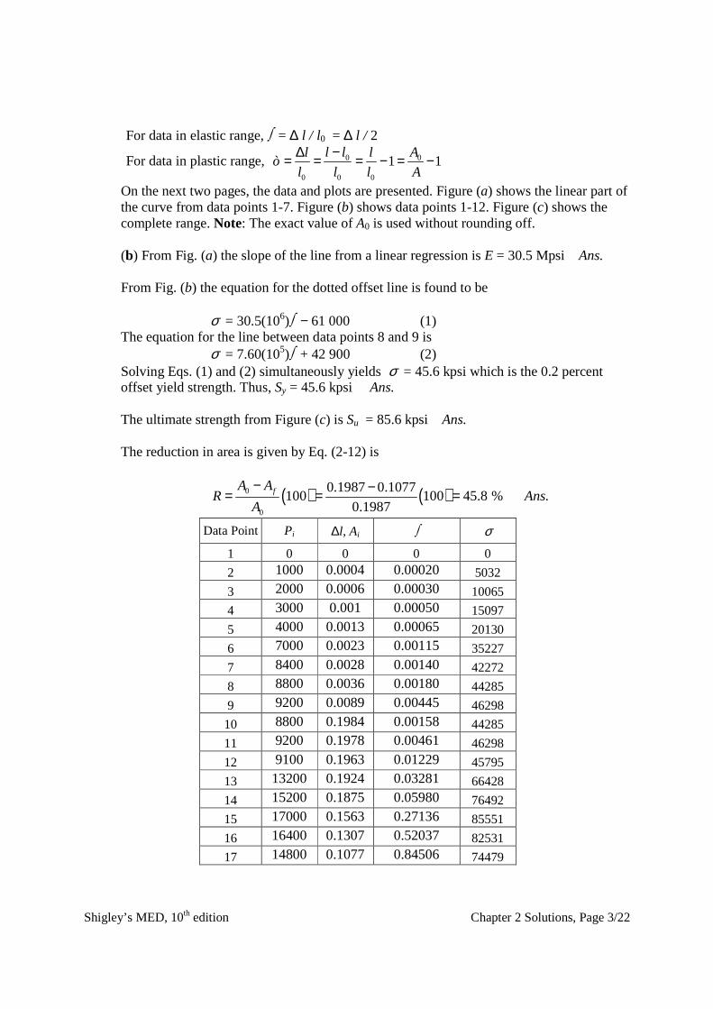
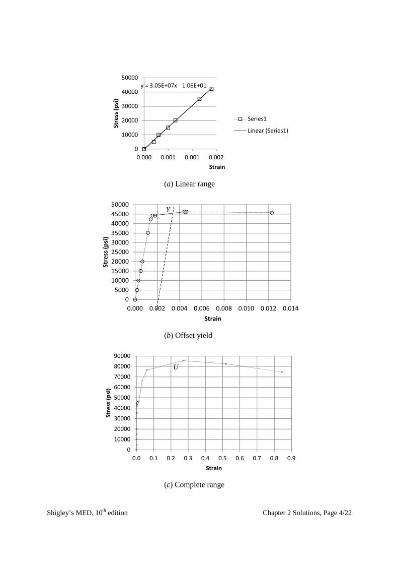
On the next two pages, the data and plots are presented. Figure (a) shows the linear part of the curve from data points 1-7. Figure (b) shows data points 1-12. Figure (c) shows the complete range. Note: The exact value of A0 is used without rounding off.

(b) From Fig. (a) the slope of the line from a linear regression is E = 30.5 Mpsi Ans. From Fig. (b) the equation for the dotted offset line is found to be σ = 30.5(106)∫ − 61 000 (1) The equation for the line between data points 8 and 9 is σ = 7.60(105)∫ + 42 900 (2) Solving Eqs. (1) and (2) simultaneously yields σ = 45.6 kpsi which is the 0.2 percent

offset yield strength. Thus, Sy = 45.6 kpsi Ans. The ultimate strength from Figure (c) is Su = 85.6 kpsi Ans. The reduction in area is given by Eq. (2-12) is

( ) ( )0

0

0.1987 0.1077100 100 45.8 % .

0.1987fA A

R AnsA

− −= = =

Data Point Pi ∆l, Ai ∫ σ 1 0 0 0 0

2 1000 0.0004 0.00020 5032

3 2000 0.0006 0.00030 10065

4 3000 0.001 0.00050 15097

5 4000 0.0013 0.00065 20130

6 7000 0.0023 0.00115 35227

7 8400 0.0028 0.00140 42272

8 8800 0.0036 0.00180 44285

9 9200 0.0089 0.00445 46298

10 8800 0.1984 0.00158 44285

11 9200 0.1978 0.00461 46298

12 9100 0.1963 0.01229 45795

13 13200 0.1924 0.03281 66428

14 15200 0.1875 0.05980 76492

15 17000 0.1563 0.27136 85551

16 16400 0.1307 0.52037 82531

17 14800 0.1077 0.84506 74479


(a) Linear range

(b) Offset yield

(c) Complete range

y = 3.05E+07x - 1.06E+01

0

10000

20000

30000

40000

50000

0.000 0.001 0.001 0.002

Str

ess

(p

si)

Strain

Series1

Linear (Series1)

0

5000

10000

15000

20000

25000

30000

35000

40000

45000

50000

0.000 0.002 0.004 0.006 0.008 0.010 0.012 0.014

Str

ess

(p

si)

Strain

Y

0

10000

20000

30000

40000

50000

60000

70000

80000

90000

0.0 0.1 0.2 0.3 0.4 0.5 0.6 0.7 0.8 0.9

Str

ess

(p

si)

Strain

U


(c) The material is ductile since there is a large amount of deformation beyond yield. (d) The closest material to the values of Sy, Sut, and R is SAE 1045 HR with Sy = 45 kpsi,

Sut = 82 kpsi, and R = 40 %. Ans. ______________________________________________________________________________ 2-7 To plot σ true vs.ε, the following equations are applied to the data.

true

P

Aσ =

Eq. (2-4)

0

0

ln for 0 0.0028 in (0 8400 lbf )

ln for 0.0028 in ( 8400 lbf )

ll P

l

Al P

A

ε

ε

= ≤ ∆ ≤ ≤ ≤

= ∆ > >

where 2

20

(0.503)0.1987 in

4A

π= =

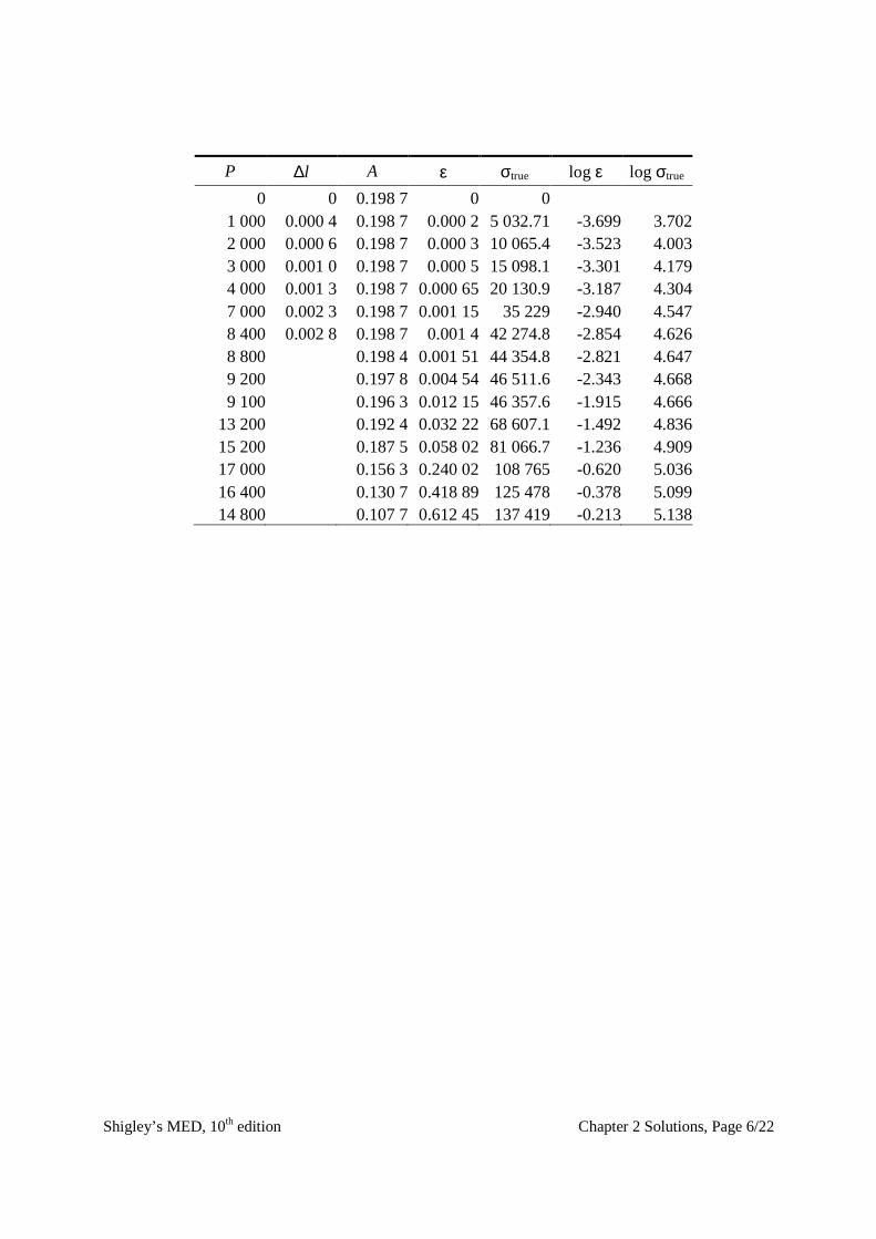
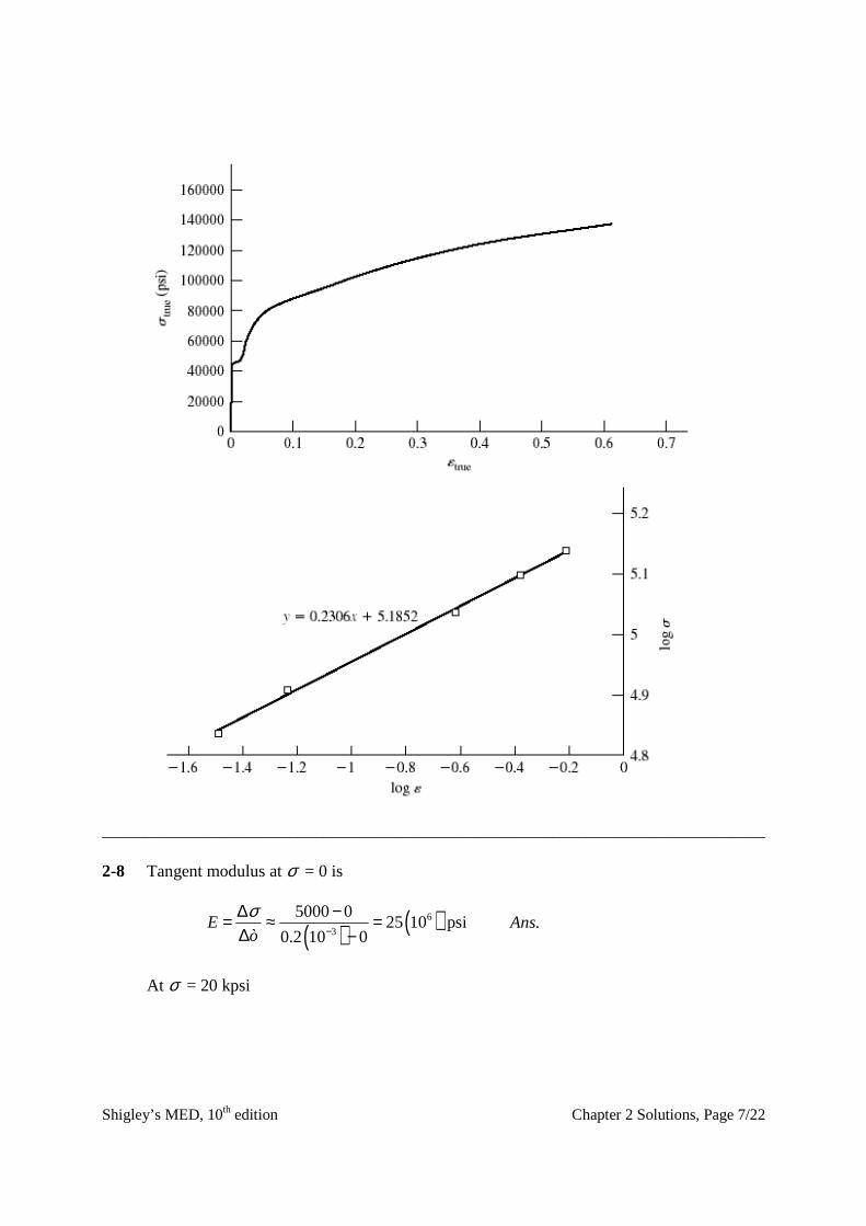
The results are summarized in the table below and plotted on the next page. The last 5 points of data are used to plot log σ vs log ε

The curve fit gives m = 0.2306

log σ0 = 5.1852 ⇒ σ0 = 153.2 kpsi Ans. For 20% cold work, Eq. (2-14) and Eq. (2-17) give,

A = A0 (1 – W) = 0.1987 (1 – 0.2) = 0.1590 in2

0

0.23060

0.1987ln ln 0.2231

0.1590

Eq. (2-18): 153.2(0.2231) 108.4 kpsi .

Eq. (2-19), with 85.6 from Prob. 2-6,

85.6107 kpsi .

1 1 0.2

my

u

uu

A

A

S Ans

S

SS Ans

W

ε

σ ε′

= = =

= = =

=

′ = = =− −


P ∆l A ε σtrue log ε log σtrue

0 0 0.198 7 0 01 000 0.000 4 0.198 7 0.000 2 5 032.71 -3.699 3.702 2 000 0.000 6 0.198 7 0.000 3 10 065.4 -3.523 4.003 3 000 0.001 0 0.198 7 0.000 5 15 098.1 -3.301 4.179 4 000 0.001 3 0.198 7 0.000 65 20 130.9 -3.187 4.304 7 000 0.002 3 0.198 7 0.001 15 35 229 -2.940 4.547 8 400 0.002 8 0.198 7 0.001 4 42 274.8 -2.854 4.626 8 800 0.198 4 0.001 51 44 354.8 -2.821 4.647 9 200 0.197 8 0.004 54 46 511.6 -2.343 4.668 9 100 0.196 3 0.012 15 46 357.6 -1.915 4.666

13 200 0.192 4 0.032 22 68 607.1 -1.492 4.836 15 200 0.187 5 0.058 02 81 066.7 -1.236 4.909 17 000 0.156 3 0.240 02 108 765 -0.620 5.036 16 400 0.130 7 0.418 89 125 478 -0.378 5.099 14 800 0.107 7 0.612 45 137 419 -0.213 5.138


______________________________________________________________________________ 2-8 Tangent modulus at σ = 0 is

( ) ( )6

3

5000 025 10 psi

0.2 10 0E

σ−

∆ −= ≈ =∆ −ò

Ans.

At σ = 20 kpsi

Shigley’s MED, 10th edition

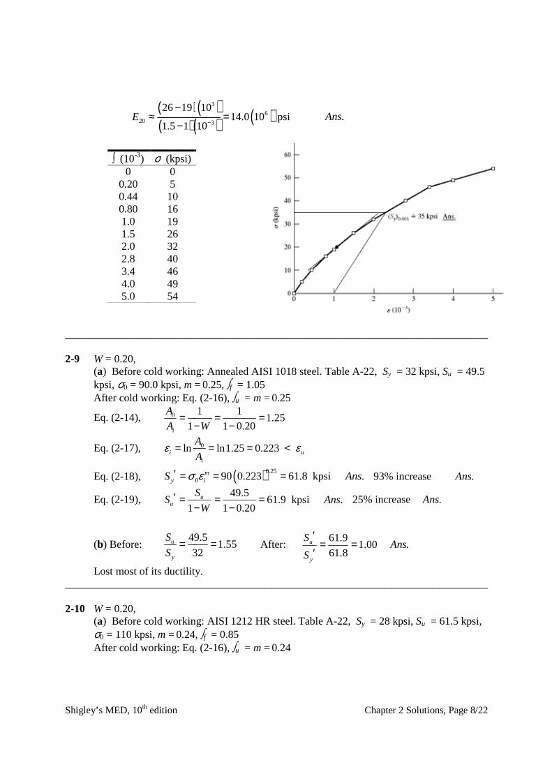
( )( )(20

26 19 10

1.5 1 10E

−≈ =

−

∫ (10-3) σ (kpsi) 0 0

0.20 5 0.44 10 0.80 16 1.0 19 1.5 26 2.0 32 2.8 40 3.4 46 4.0 49 5.0 54

______________________________________________________________________________ 2-9 W = 0.20, (a) Before cold working:

kpsi, σ0 = 90.0 kpsi, m After cold working: Eq. (2

Eq. (2-14), 0

1 1 0.20i

A

A W= = =

− −

Eq. (2-17), ln ln1.25 0.223i uε ε= = = <

Eq. (2-18), y iS Ansσ ε′ = = =

Eq. (2-19), 1 1 0.20uS Ans′ = = =

− −

(b) Before: 49.5

32u

y

S

S= =

Lost most of its ductility______________________________________________________________________________ 2-10 W = 0.20, (a) Before cold working: AISI 1212 HR steel. Table A

σ0 = 110 kpsi, m = 0.24, After cold working: Eq. (2

Chapter 2

)( )( ) ( )

3

6

3

26 19 1014.0 10 psi

1.5 1 10−≈ = Ans.

______________________________________________________________________________

) Before cold working: Annealed AISI 1018 steel. Table A-22, Sy

= 0.25, ∫f = 1.05 After cold working: Eq. (2-16), ∫u = m = 0.25

1 11.25

1 1 0.20A W= = =

− −

0ln ln1.25 0.223i ui

A

Aε ε= = = <

( )0.25

0 90 0.223 61.8 kpsi .my iS Ansσ ε= = = 93% increase

49.561.9 kpsi .

1 1 0.20uS

S AnsW

= = =− −

25% increase

49.51.55

32= = After:

61.91.00

61.8u

y

S

S

′= =

′

ductility. ______________________________________________________________________________

) Before cold working: AISI 1212 HR steel. Table A-22, Sy = 28 kpsi, 0.24, ∫f = 0.85

q. (2-16), ∫u = m = 0.24

Chapter 2 Solutions, Page 8/22

______________________________________________________________________________

y = 32 kpsi, Su = 49.5

93% increase Ans.

25% increase Ans.

Ans.

______________________________________________________________________________

= 28 kpsi, Su = 61.5 kpsi,


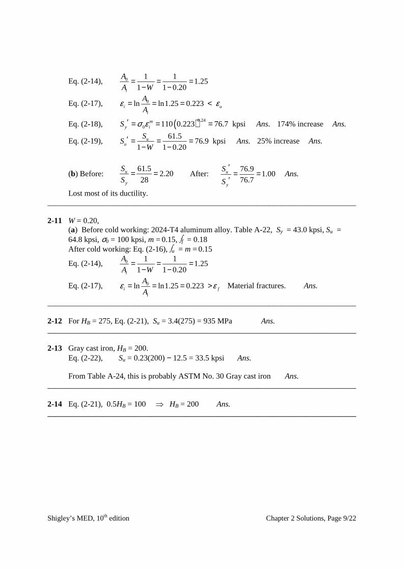
Eq. (2-14), 0 1 11.25

1 1 0.20i

A

A W= = =

− −

Eq. (2-17), 0ln ln1.25 0.223i ui

A

Aε ε= = = <

Eq. (2-18), ( )0.24

0 110 0.223 76.7 kpsi .my iS Ansσ ε′ = = = 174% increase Ans.

Eq. (2-19), 61.5

76.9 kpsi .1 1 0.20

uu

SS Ans

W′ = = =

− − 25% increase Ans.

(b) Before: 61.5

2.2028

u

y

S

S= = After:

76.91.00

76.7u

y

S

S

′= =

′ Ans.

Lost most of its ductility. ______________________________________________________________________________ 2-11 W = 0.20, (a) Before cold working: 2024-T4 aluminum alloy. Table A-22, Sy = 43.0 kpsi, Su =

64.8 kpsi, σ0 = 100 kpsi, m = 0.15, ∫f = 0.18 After cold working: Eq. (2-16), ∫u = m = 0.15

Eq. (2-14), 0 1 11.25

1 1 0.20i

A

A W= = =

− −

Eq. (2-17), 0ln ln1.25 0.223i fi

A

Aε ε= = = > Material fractures. Ans.

______________________________________________________________________________ 2-12 For HB = 275, Eq. (2-21), Su = 3.4(275) = 935 MPa Ans. ______________________________________________________________________________ 2-13 Gray cast iron, HB = 200. Eq. (2-22), Su = 0.23(200) − 12.5 = 33.5 kpsi Ans. From Table A-24, this is probably ASTM No. 30 Gray cast iron Ans. ______________________________________________________________________________ 2-14 Eq. (2-21), 0.5HB = 100 ⇒ HB = 200 Ans. ______________________________________________________________________________


2-15 For the data given, converting HB to Su using Eq. (2-21)

HB Su (kpsi) Su2 (kpsi)

230 115

13225

232 116

13456

232 116

13456

234 117

13689

235 117.5

13806.25

235 117.5

13806.25

235 117.5

13806.25

236 118

13924

236 118

13924

239 119.5

14280.25

ΣSu = 1172 ΣSu2 = 137373

Eq. (1-6)

1172

117.2 117 kpsi .10

uu

SS Ans

N= = = ≈∑

Eq. (1-7),

( )

102 2

2

1137373 10 117.2

1.27 kpsi .1 9u

u ui

S

S NSs Ans

N=

− −= = =

−

∑

______________________________________________________________________________ 2-16 For the data given, converting HB to Su using Eq. (2-22)

HB Su (kpsi) Su2 (kpsi)

230 40.4

1632.16

232 40.86

1669.54

232 40.86

1669.54

234 41.32

1707.342

235 41.55

1726.403

235 41.55

1726.403

235 41.55

1726.403

236 41.78

1745.568

236 41.78

1745.568

239 42.47

1803.701

ΣSu = 414.12 ΣSu2 = 17152.63


Eq. (1-6)

414.12

41.4 kpsi .10

uu

SS Ans

N= = =∑

Eq. (1-7),

( )

102 2

2

117152.63 10 41.4

1.20 .1 9u

u ui

S

S NSs Ans

N=

− −= = =

−

∑

______________________________________________________________________________

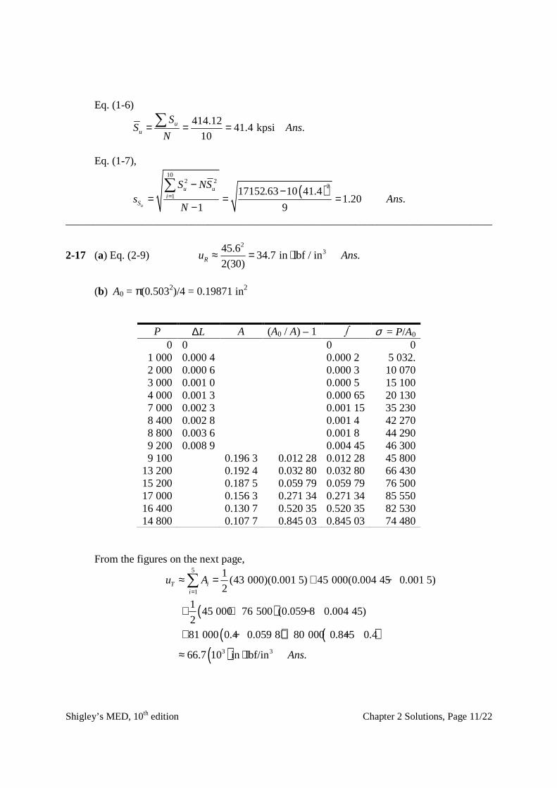
2-17 (a) Eq. (2-9) 2

345.634.7 in lbf / in .

2(30)Ru Ans≈ = ⋅

(b) A0 = π(0.5032)/4 = 0.19871 in2

P ∆L A (A0 / A) – 1 ∫ σ = P/A0 0 0 0 0

1 000 0.000 4 0.000 2 5 032. 2 000 0.000 6 0.000 3 10 070 3 000 0.001 0 0.000 5 15 100 4 000 0.001 3 0.000 65 20 130 7 000 0.002 3 0.001 15 35 230 8 400 0.002 8 0.001 4 42 270 8 800 0.003 6 0.001 8 44 290 9 200 0.008 9 0.004 45 46 300 9 100 0.196 3 0.012 28 0.012 28 45 800

13 200 0.192 4 0.032 80 0.032 80 66 430 15 200 0.187 5 0.059 79 0.059 79 76 500 17 000 0.156 3 0.271 34 0.271 34 85 550 16 400 0.130 7 0.520 35 0.520 35 82 530 14 800 0.107 7 0.845 03 0.845 03 74 480

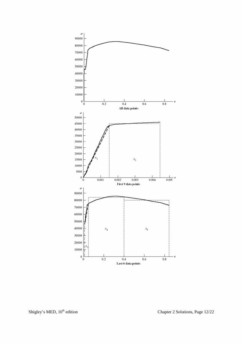
From the figures on the next page,

( )( ) ( )

( )

5

1

3 3

1(43 000)(0.001 5) 45 000(0.004 45 0.001 5)

2

145 000 76 500 (0.059 8 0.004 45)

281 000 0.4 0.059 8 80 000 0.845 0.4

66.7 10 in lbf/in .

T ii

u A

Ans

=

≈ = + −

+ + −

+ − + −

≈ ⋅

∑

Shigley’s MED, 10th edition

Chapter 2

Chapter 2 Solutions, Page 12/22


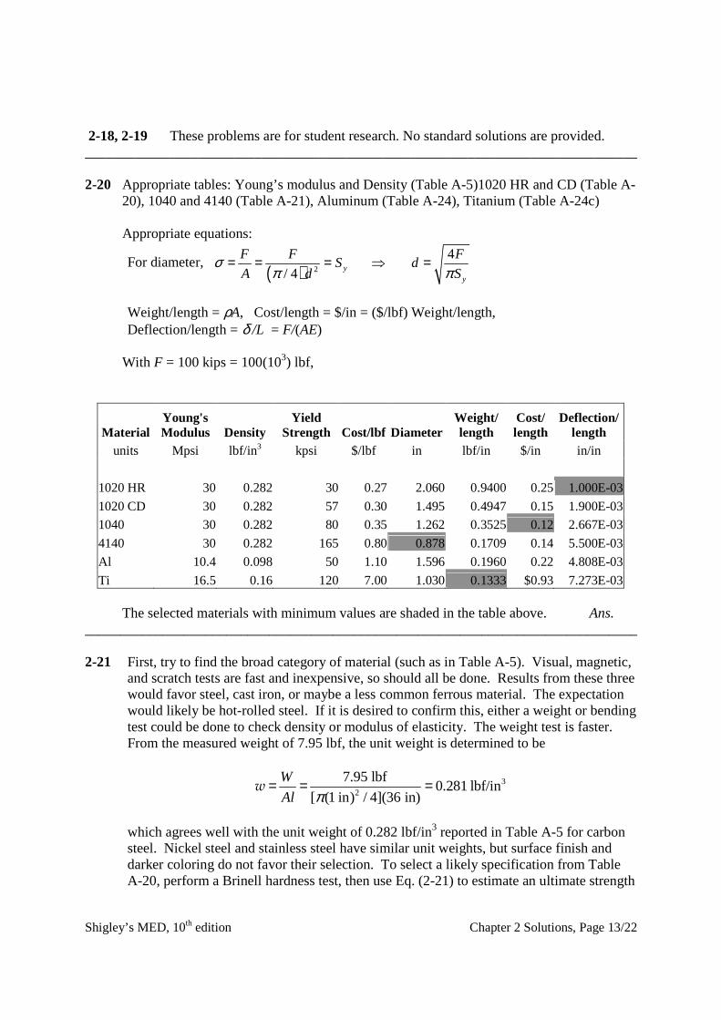
2-18, 2-19 These problems are for student research. No standard solutions are provided. ______________________________________________________________________________ 2-20 Appropriate tables: Young’s modulus and Density (Table A-5)1020 HR and CD (Table A-

20), 1040 and 4140 (Table A-21), Aluminum (Table A-24), Titanium (Table A-24c) Appropriate equations:

For diameter, ( ) 2

4

/ 4 yy

F F FS d

A d Sσ

π π= = = ⇒ =

Weight/length = ρA, Cost/length = $/in = ($/lbf) Weight/length, Deflection/length = δ /L = F/(AE) With F = 100 kips = 100(103) lbf,

Material Young's Modulus Density

Yield Strength Cost/lbf Diameter

Weight/ length

Cost/ length

Deflection/ length

units Mpsi lbf/in3 kpsi $/lbf in lbf/in $/in in/in

1020 HR 30 0.282 30 0.27 2.060 0.9400 0.25 1.000E-03

1020 CD 30 0.282 57 0.30 1.495 0.4947 0.15 1.900E-03

1040 30 0.282 80 0.35 1.262 0.3525 0.12 2.667E-03

4140 30 0.282 165 0.80 0.878 0.1709 0.14 5.500E-03

Al 10.4 0.098 50 1.10 1.596 0.1960 0.22 4.808E-03

Ti 16.5 0.16 120 7.00 1.030 0.1333 $0.93 7.273E-03 The selected materials with minimum values are shaded in the table above. Ans. ______________________________________________________________________________ 2-21 First, try to find the broad category of material (such as in Table A-5). Visual, magnetic,

and scratch tests are fast and inexpensive, so should all be done. Results from these three would favor steel, cast iron, or maybe a less common ferrous material. The expectation would likely be hot-rolled steel. If it is desired to confirm this, either a weight or bending test could be done to check density or modulus of elasticity. The weight test is faster. From the measured weight of 7.95 lbf, the unit weight is determined to be

32

7.95 lbf0.281 lbf/in

[ (1 in) / 4](36 in)

W

Al π= = =w

which agrees well with the unit weight of 0.282 lbf/in3 reported in Table A-5 for carbon steel. Nickel steel and stainless steel have similar unit weights, but surface finish and darker coloring do not favor their selection. To select a likely specification from Table A-20, perform a Brinell hardness test, then use Eq. (2-21) to estimate an ultimate strength


of 0.5 0.5(200) 100 kpsiu BS H= = = . Assuming the material is hot-rolled due to the

rough surface finish, appropriate choices from Table A-20 would be one of the higher carbon steels, such as hot-rolled AISI 1050, 1060, or 1080. Ans.

______________________________________________________________________________ 2-22 First, try to find the broad category of material (such as in Table A-5). Visual, magnetic,

and scratch tests are fast and inexpensive, so should all be done. Results from these three favor a softer, non-ferrous material like aluminum. If it is desired to confirm this, either a weight or bending test could be done to check density or modulus of elasticity. The weight test is faster. From the measured weight of 2.90 lbf, the unit weight is determined to be

32

2.9 lbf0.103 lbf/in

[ (1 in) / 4](36 in)

W

Al π= = =w

which agrees reasonably well with the unit weight of 0.098 lbf/in3 reported in Table A-5 for aluminum. No other materials come close to this unit weight, so the material is likely aluminum. Ans.

______________________________________________________________________________ 2-23 First, try to find the broad category of material (such as in Table A-5). Visual, magnetic,

and scratch tests are fast and inexpensive, so should all be done. Results from these three favor a softer, non-ferrous copper-based material such as copper, brass, or bronze. To further distinguish the material, either a weight or bending test could be done to check density or modulus of elasticity. The weight test is faster. From the measured weight of 9 lbf, the unit weight is determined to be

32

9.0 lbf0.318 lbf/in

[ (1 in) / 4](36 in)

W

Al π= = =w

which agrees reasonably well with the unit weight of 0.322 lbf/in3 reported in Table A-5 for copper. Brass is not far off (0.309 lbf/in3), so the deflection test could be used to gain additional insight. From the measured deflection and utilizing the deflection equation for an end-loaded cantilever beam from Table A-9, Young’s modulus is determined to be

( )

( )33

4

100 2417.7 Mpsi

3 3 (1) 64 (17 / 32)

FlE

Iy π= = =

which agrees better with the modulus for copper (17.2 Mpsi) than with brass (15.4 Mpsi). The conclusion is that the material is likely copper. Ans.

______________________________________________________________________________ 2-24 and 2-25 These problems are for student research. No standard solutions are provided. ______________________________________________________________________________ 2-26 For strength, σ = F/A = S ⇒ A = F/S


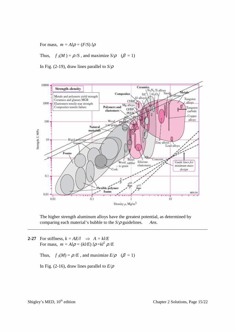
For mass, m = Alρ = (F/S) lρ Thus, f 3(M ) = ρ /S , and maximize S/ρ (β = 1) In Fig. (2-19), draw lines parallel to S/ρ

The higher strength aluminum alloys have the greatest potential, as determined by

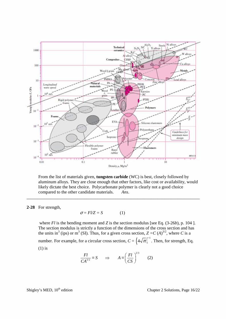
comparing each material’s bubble to the S/ρ guidelines. Ans. ______________________________________________________________________________ 2-27 For stiffness, k = AE/l ⇒ A = kl/E For mass, m = Alρ = (kl/E) lρ =kl2 ρ /E Thus, f 3(M) = ρ /E , and maximize E/ρ (β = 1) In Fig. (2-16), draw lines parallel to E/ρ


From the list of materials given, tungsten carbide (WC) is best, closely followed by

aluminum alloys. They are close enough that other factors, like cost or availability, would likely dictate the best choice. Polycarbonate polymer is clearly not a good choice compared to the other candidate materials. Ans.

______________________________________________________________________________ 2-28 For strength, σ = Fl/Z = S (1) where Fl is the bending moment and Z is the section modulus [see Eq. (3-26b), p. 104 ].

The section modulus is strictly a function of the dimensions of the cross section and has the units in3 (ips) or m3 (SI). Thus, for a given cross section, Z =C (A)3/2, where C is a

number. For example, for a circular cross section, C = ( ) 1

4 π−

. Then, for strength, Eq.

(1) is

2/3

3/2

Fl FlS A

CA CS = ⇒ =

(2)


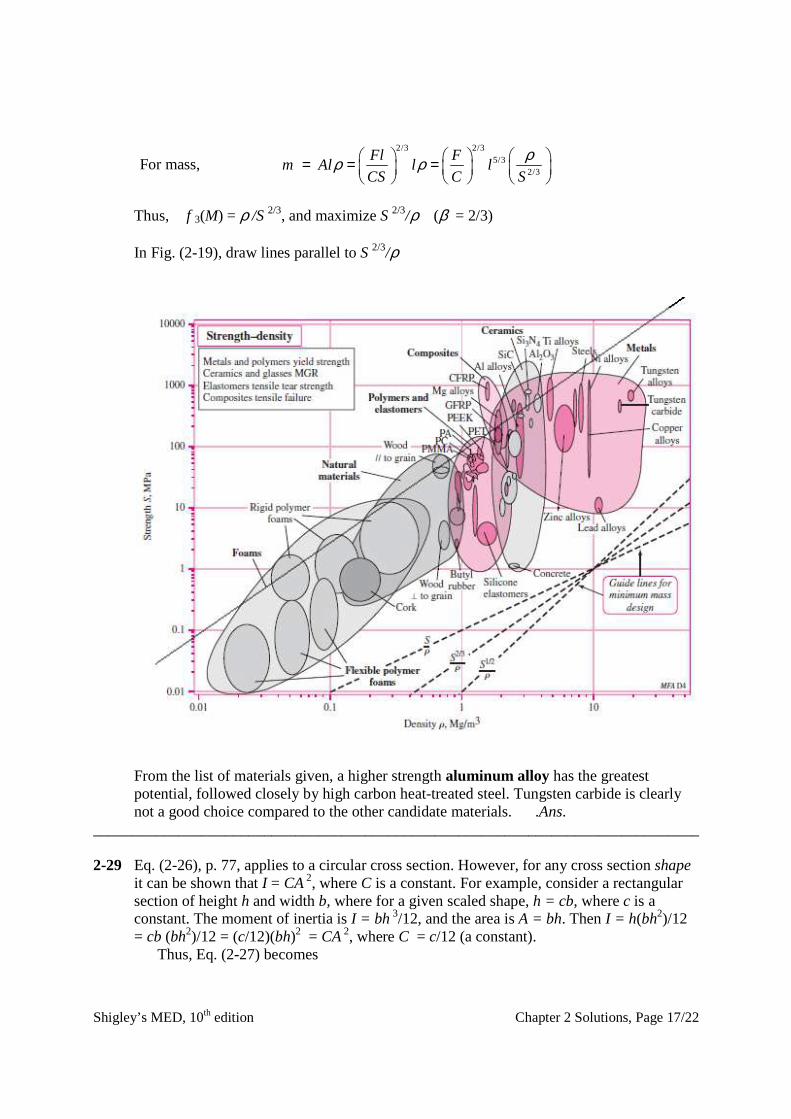
For mass, 2/3 2/3

5/32/3

Fl F

m Al l lCS C S

ρρ ρ = = =

Thus, f 3(M) = ρ /S 2/3, and maximize S 2/3/ρ (β = 2/3) In Fig. (2-19), draw lines parallel to S 2/3/ρ

From the list of materials given, a higher strength aluminum alloy has the greatest

potential, followed closely by high carbon heat-treated steel. Tungsten carbide is clearly not a good choice compared to the other candidate materials. .Ans.

______________________________________________________________________________ 2-29 Eq. (2-26), p. 77, applies to a circular cross section. However, for any cross section shape

it can be shown that I = CA 2, where C is a constant. For example, consider a rectangular section of height h and width b, where for a given scaled shape, h = cb, where c is a constant. The moment of inertia is I = bh 3/12, and the area is A = bh. Then I = h(bh2)/12 = cb (bh2)/12 = (c/12)(bh)2 = CA 2, where C = c/12 (a constant).

Thus, Eq. (2-27) becomes


1/23

3

klA

CE

=

and Eq. (2-29) becomes

1/2

5/21/23

km Al l

C E

ρρ = =

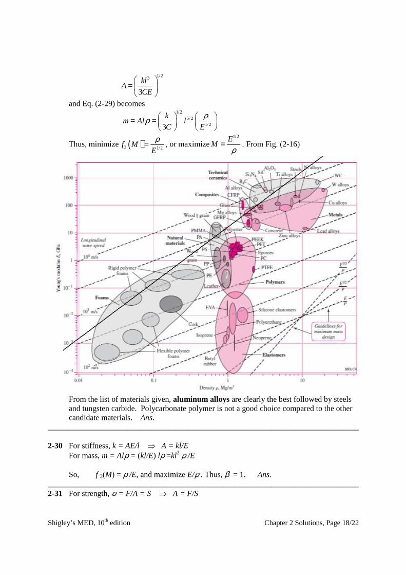
Thus, minimize ( )3 1/2f M

E

ρ= , or maximize1/2E

Mρ

= . From Fig. (2-16)

From the list of materials given, aluminum alloys are clearly the best followed by steels

and tungsten carbide. Polycarbonate polymer is not a good choice compared to the other candidate materials. Ans.

______________________________________________________________________________ 2-30 For stiffness, k = AE/l ⇒ A = kl/E For mass, m = Alρ = (kl/E) lρ =kl2 ρ /E So, f 3(M) = ρ /E, and maximize E/ρ . Thus, β = 1. Ans. ______________________________________________________________________________ 2-31 For strength, σ = F/A = S ⇒ A = F/S


For mass, m = Alρ = (F/S) lρ So, f 3(M ) = ρ /S, and maximize S/ρ . Thus, β = 1. Ans. ______________________________________________________________________________ 2-32 Eq. (2-26), p. 77, applies to a circular cross section. However, for any cross section shape

it can be shown that I = CA 2, where C is a constant. For the circular cross section (see p.77), C = (4π)−1. Another example, consider a rectangular section of height h and width b, where for a given scaled shape, h = cb, where c is a constant. The moment of inertia is

I = bh 3/12, and the area is A = bh. Then I = h(bh2)/12 = cb (bh2)/12 = (c/12)(bh)2 = CA 2, where C = c/12, a constant.

Thus, Eq. (2-27) becomes

1/23

3

klA

CE

=

and Eq. (2-29) becomes

1/2

5/21/23

km Al l

C E

ρρ = =

So, minimize ( )3 1/2f M

E

ρ= , or maximize1/2E

Mρ

= . Thus, β = 1/2. Ans.

______________________________________________________________________________ 2-33 For strength, σ = Fl/Z = S (1) where Fl is the bending moment and Z is the section modulus [see Eq. (3-26b), p. 104 ].

The section modulus is strictly a function of the dimensions of the cross section and has the units in3 (ips) or m3 (SI). The area of the cross section has the units in2 or m2. Thus, for a given cross section, Z =C (A)3/2, where C is a number. For example, for a circular cross

section, Z = πd 3/(32)and the area is A = πd 2/4. This leads to C =( ) 1

4 π−

. So, with

Z =C (A)3/2, for strength, Eq. (1) is

2/3

3/2

Fl FlS A

CA CS = ⇒ =

(2)

For mass, 2/3 2/3

5/32/3

Fl F

m Al l lCS C S

ρρ ρ = = =

So, f 3(M) = ρ /S 2/3, and maximize S 2/3/ρ. Thus, β = 2/3. Ans. ______________________________________________________________________________


2-34 For stiffness, k=AE/l, or, A = kl/E. Thus, m = ρAl =ρ (kl/E )l = kl 2 ρ /E. Then, M = E /ρ and β = 1. From Fig. 2-16, lines parallel to E /ρ for ductile materials include steel, titanium,

molybdenum, aluminum alloys, and composites. For strength, S = F/A, or, A = F/S. Thus, m = ρAl =ρ F/Sl = Fl ρ /S. Then, M = S/ρ and β = 1. From Fig. 2-19, lines parallel to S/ρ give for ductile materials, steel, aluminum alloys,

nickel alloys, titanium, and composites. Common to both stiffness and strength are steel, titanium, aluminum alloys, and

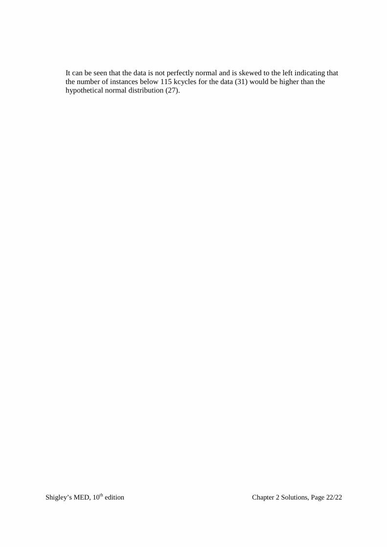
composites. Ans. ______________________________________________________________________________ 2-35 See Prob. 1-13 solution for x = 122.9 kcycles and xs = 30.3 kcycles. Also, in that solution

it is observed that the number of instances less than 115 kcycles predicted by the normal distribution is 27; whereas, the data indicates the number to be 31.

From Eq. (1-4), the probability density function (PDF), with xµ = and ˆ xsσ = , is

2 2

1 1 1 1 122.9( ) exp exp

2 2 30.32 30.3 2xx

x x xf x

ss π π

− − = − = −

(1)

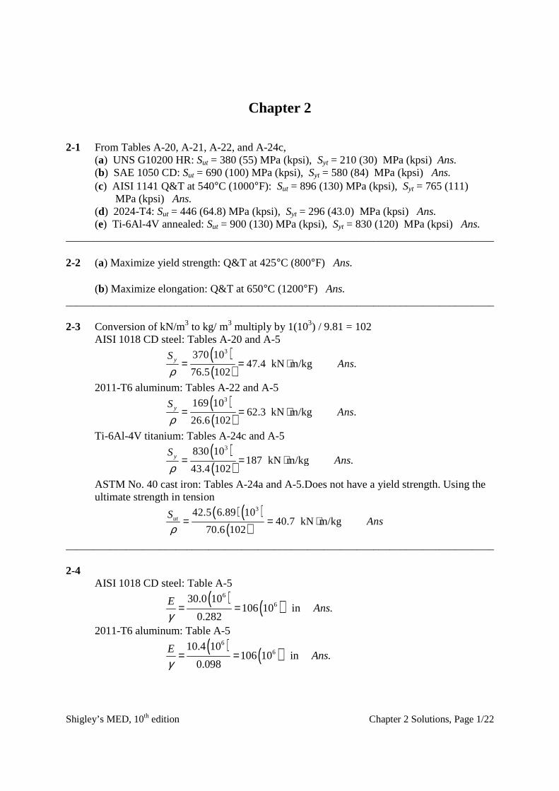
The discrete PDF is given by f /(Nw), where N = 69 and w = 10 kcycles. From the Eq. (1)

and the data of Prob. 1-13, the following plots are obtained.


Range midpoint (kcycles) Frequency

Observed PDF

Normal PDF

x f f /(Nw) f (x) 60 2 0.002898551 0.001526493 70 1 0.001449275 0.002868043 80 3 0.004347826 0.004832507 90 5 0.007246377 0.007302224 100 8 0.011594203 0.009895407 110 12 0.017391304 0.012025636 120 6 0.008695652 0.013106245 130 10 0.014492754 0.012809861 140 8 0.011594203 0.011228104 150 5 0.007246377 0.008826008 160 2 0.002898551 0.006221829 170 3 0.004347826 0.003933396 180 2 0.002898551 0.002230043 190 1 0.001449275 0.001133847 200 0 0 0.000517001 210 1 0.001449275 0.00021141

Plots of the PDF’s are shown below.

0

0.002

0.004

0.006

0.008

0.01

0.012

0.014

0.016

0.018

0.02

0 20 40 60 80 100 120 140 160 180 200 220

Normal Distribution

Histogram

L (kcycles)

Pro

ba

bil

ity

De

nsi

ty


It can be seen that the data is not perfectly normal and is skewed to the left indicating that the number of instances below 115 kcycles for the data (31) would be higher than the hypothetical normal distribution (27).

Documents

Chapter 2latcha/me486/BN10/Chap02_10e.pdf · Shigley’s MED, 10 th edition Chapter 2 Solutions, Page 1/22 Chapter 2 2-1 From Tables A-20, A-21, ... 9 100 0.196 3 0.012 15 46 357.6