Chapter 2: Lasso for linear models

Statistics for High-Dimensional Data (Buhlmann & van de Geer)

Lasso Proposed by Tibshirani (1996) Least Absolute Shrinkage and Selection

Operator Why we still use it

Accurate in prediction and variable selection (under certain assumptions) and computationally feasible

2.2. Introduction and preliminaries Univariate response Yi

Covariate vector Xi

Can be fixed or random variables Typically independence assumed, but Lasso

can be applied to correlated data For simplicity, we can assume the intercept is

zero and all covariates are centered and measured on the same scale Standardization

2.2.1. The Lasso estimator

“Shrunken” least squares estimator βj=0 for some j Convex optimization – computationally efficient

Equivalent to solving:

For some R (data-dependent 1:1 correspondence between R and λ) Estimating the variance

Can use residual sum of squares and df of Lasso Or we can estimate β and σ2 simultaneously (Ch. 9)

2.3. Orthonormal design p=n and n-1XTX=Ipxp

Then:

2.4. Prediction Often cross-validation used to choose the λ

minimizing the squared-error risk Cross-validation can also be used to assess the

predictive accuracy Some asymptotics (more in Ch. 6)

For high-dimensional scenarios (allowing p to depend on n)

For consistency, we assume sparsity

Then:

2.5. Variable screening Under certain assumptions including (true) model sparsity

and conditions on the design matrix (Thm. 7.1), for a suitable range of λ,

For q=1,2; derivation in Ch. 6

We can use the Lasso estimate as variable screening:

Variables with non-zero coefficients remain the same across different solutions (>1 solution for non-convex optimization such as when p>n)

The number of variables estimated as non-zero doesn’t exceed min(n,p)

And

Lemma 2.1. and tuning parameter selection

Tuning parameter selection For prediction, smaller λ is preferred, while larger

penalty is needed for good variable selection (discussed more in Ch. 10-11)

The smaller λ tuned from CV can be utilized for the screening process

2.6. Variable selection AIC and BIC use the l0-norm as a penalty

Computation is infeasible for any relatively large p, since the objective function using this norm is non-convex

For The set of all Lasso sub-models denoted by:

Then and We want to know whether is

contained in and if so, which value of λ will identify S0

With a “neighborhood stability” assumption on X (more later) and assuming Then for

2.6.1. Neighborhood stability and irrepresentable condition In order for consistency of Lasso’s variable selection, we

make assumptions about X WLOG, let the first s0 variables form the active set S0

Let

Then the irrepresentable condition is:

Above is sufficient condition for consistency of Lasso model selection; RHS is “<=1” for necessary condition

This is easier to represent than the neighborhood stability condition but the two are equivalent for

Essentially consistency fails under too much linear dependence within sub-matrices of X

Summary of some Lasso properties (Table 2.2)

2.8. Adaptive Lasso Two-stage procedure instead of just using l1-

penalty:

Lasso can be used for the initial estimation, with CV for λ tuning, followed by the same procedure for the second stage

The adaptive Lasso gives a small penalty to βj with initial estimates of large magnitude

2.8.1. Illustration: simulated data 1000 variables, 3 of which have true signal; “medium-

sized” signal-to-noise ratio

Both selected the active set, but adaptive Lasso selects only 10 noise variables as opposed to 41 for the Lasso

2.8.2. Orthonormal design For

Then:

2.8.3. The adaptive Lasso: variable selection under weak conditions For consistency of variable selection of the

adaptive Lasso, we need large enough non-zero coefficients:

But we can assume weaker conditions than the neighborhood stability (irrepresentable) condition on the design matrix required for consistency of the Lasso (more in Ch. 7)

Then:

2.8.4. Computation We can reparameterize into a Lasso problem:

Then the objective function is:

If a solution to this is , then the solution for the adaptive Lasso is given by:

Any algorithm for computing Lasso estimates can be used to compute the adaptive Lasso (more on algorithms later)

2.8.5. Multi-step adaptive Lasso Procedure as follows:

2.8.6. Non-convex penalty functions General penalized linear regression:

Ex: SCAD (Smoothly Clipped Absolute Deviation)

Non-differentiable at zero and non-convex SCAD is related to the multi-step weighted Lasso:

Another non-convex penalty function commonly used is the lr-norm for r close to zero (Ch. 6-7)

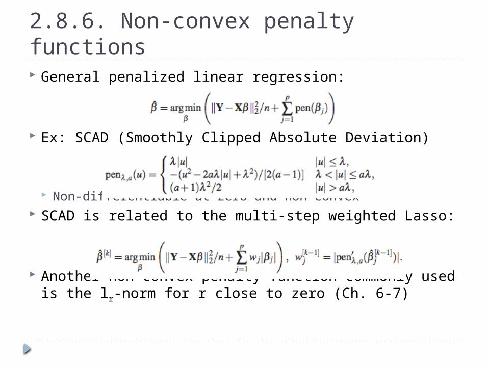
2.9. Thresholding the Lasso If we want a sparser model, instead of the adaptive

Lasso we can threshold the Lasso estimates:

Then we can refit the model (via OLS) for the non-zero estimates:

Theoretical properties are as good as or better than the adaptive Lasso (more in Ch. 6-7)

The tuning parameters can be chosen sequentially as in the adaptive Lasso

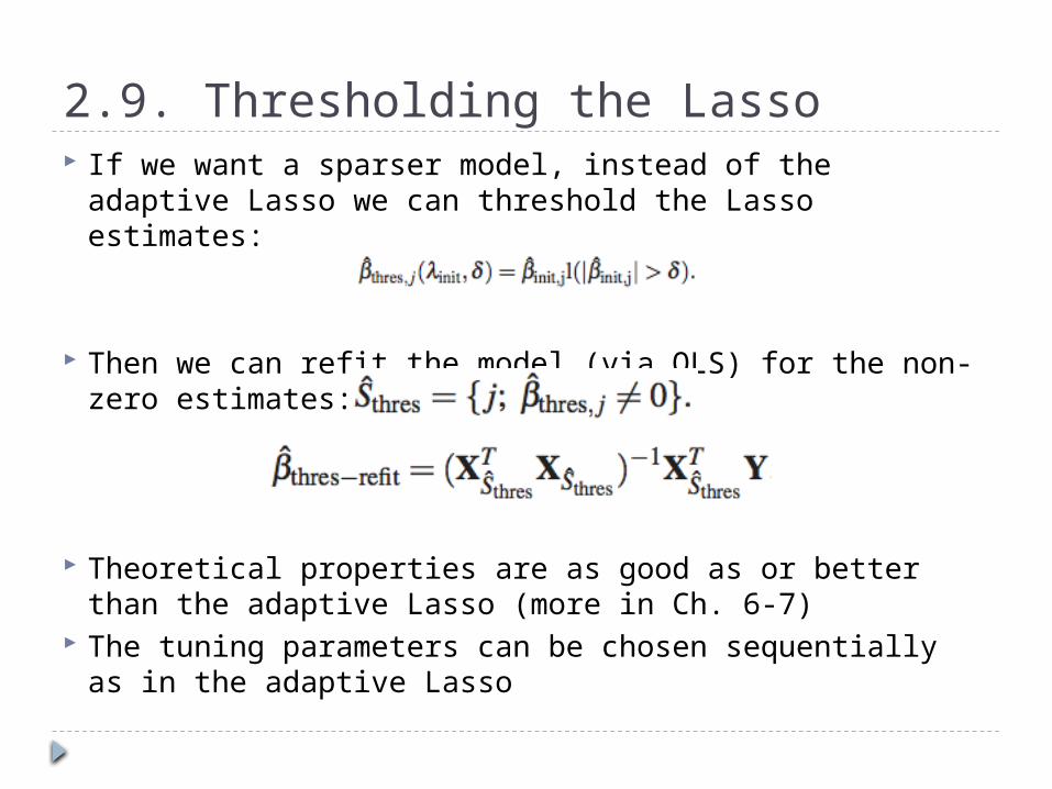
2.10. The relaxed Lasso First stage: all possible sub-models

computed (across λ) Second stage:

With smaller penalty to lessen the bias of Lasso estimation

Performs similarly to adaptive Lasso in practice

ϕ=0 yields the Lasso-OLS hybrid model Lasso first stage, OLS second stage

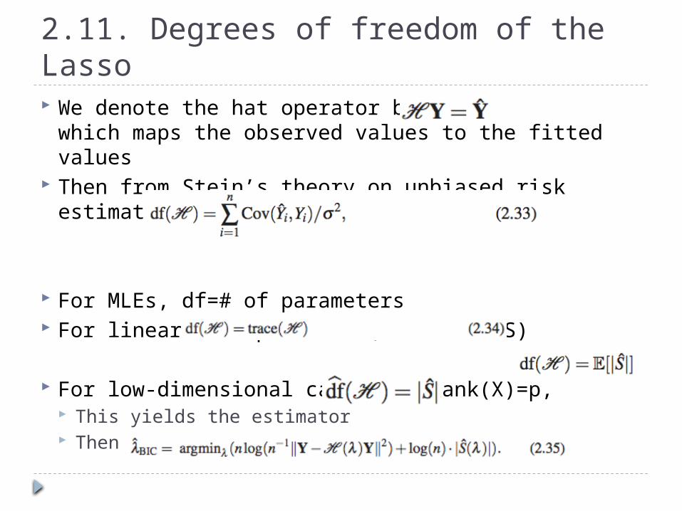
2.11. Degrees of freedom of the Lasso We denote the hat operator by which

maps the observed values to the fitted values Then from Stein’s theory on unbiased risk

estimation,

For MLEs, df=# of parameters For linear hat operators (such as OLS)

For low-dimensional case with rank(X)=p, This yields the estimator Then the BIC can be used to to select λ:

2.12. Path-following algorithms We typically want to compute the estimator for many

values of λ We can compute the entire regularized solution path

over all λ Because the solution path is piecewise linear in λ:

Typically the number of cutpoints λk are O(n). The modified LARS algorithm (Efron 2004) can be used to

construct the whole regularized solution path Exact method

2.12.1. Coordinatewise optimization and shooting algorithms For very high-dimensional problems

coordinate descent algorithms are much faster than exact methods such as the LARS algorithm With loss functions other than squared error loss,

exact methods are often not possible It is often sufficient to compute estimates over

a grid of λ values :

With such that

Optimization (continued) Let and

The update in step 4 is explicit due to squared-error loss function:

2.13. Elastic net: an extension Double-penalization version of Lasso:

After correction: This is equivalent to the Lasso under orthonormal

design