Chapter 2 Knowledge Discovery and Data Mining

Chapter 2

Knowledge Discovery and DataMining

In this chapter we recall the foundations of Data Mining. We distinguish the Knowl-edge Discovery process, a compound activity which requires user interaction, fromits Data Mining task. Data Mining in this strict interpretation is a crucial stepof the KDD process. We step through a more detailed analysis of Data Miningproblems and techniques, by presenting a general break-down of the componentsof DM algorithms, and then showing its instantiation to some common cases. Thesystematic analysis of the algorithmic components of data mining techniques is thepreliminary step to studying their parallel implementation, which is the matter ofthe next chapter.

The chapter has the following structure. Section 2.1 introduces the basic con-cept of knowledge extraction, section 2.2 discusses the duality among models andpatters in encoding knowledge. Section 2.3 describes the overall structure of theknowledge discovery process, its component steps, and the consequences on KDDsystem architecture.

The impact of the KDD process structure on data management techniques is thetopic of section 2.4. Section 2.5 is the main part of this chapter. We specify whatis a data mining problem and define data mining algorithms, identifying their fun-damental components. This taxonomy of the mining techniques is largely inspiredby the work of Hand, Mannila and Smyth [HMS01]. To instantiate the abstractconcept, the final part of the chapter describes three well-known data mining algo-rithms, k-means clustering (§ 2.6), Autoclass clustering (§ 2.7) and classification byinduction of decision trees (§ 2.8).

40 Chapter 2. Knowledge Discovery and Data Mining

2.1 Information and Knowledge

It is nowadays a commonplace to say that the ever growing size of electronic archivespushes the need to automate the interpretation of such an amount of data. Theclassical definition of Data Mining given in [FPSU96] is

Knowledge discovery in databases is the non-trivial process of identifyingvalid, novel, potentially useful, and ultimately understandable patterns indata.

This is the commonly accepted definition of data mining, even if different re-searchers shift the attention on different aspects. Data analysis is intended to beautomatic to a large extent, and patterns in this context are every kind of of unex-pected data relationships and behaviors.

Large databases contain much more information than what is apparent. Trends,patterns, regularities, relationships among seemingly unrelated variables are implicitin the data. If properly made explicit, all this kinds of information can be a greatadvantage in the industrial, economic, scientific fields just to name three.

Knowledge in the form of descriptive models, which allow understanding andpredicting phenomena, is the ultimate goal of science. On the other hand, a deeperinsight in the behavior of a social or productive system can be a great advantagein commercial activities as much as finer control on production processes can give acompetitive edge in the industrial field.

Earth observation systems, telecommunication systems, world-scale economictransfers are all examples of scientific, industrial and economic activities whosemanagement systems can daily collect a data amount in the order of the Terabyte.

It is of course no longer feasible to rely only on human intuition and innateability to recognize visual and symbolic patterns. Database size forces the analysisto be as much as possible automatic.

The field of Data Mining has originated from the application to this problem ofmethods from nearby research fields: statistics, machine learning, database theoryare some examples. The tools and algorithms from these fields have since then un-dergone an intense investigation, because their application is bounded by a numberof practical constraints.

Because of their size, datasets cannot be kept in-memory. Architectural limitsimpose that they are on secondary or even tertiary storage. The situation is notlikely to change, as the size of the archives commercially used today is several ordersof magnitude times bigger, and grows faster, than the size of main-memories.

Since datasets are out of core, the common intuition of algorithmically “tractable”problem fails. It impossible to exploit even moderately complex algorithms in theknowledge extraction from huge data sets, even O(N2) complexity is not affordablewhen speaking about Terabytes of data. Simple algorithms have often to be dis-carded, or recoded, to mitigate the penalty incurred when working on data that isat the bottom of a deep memory hierarchy (see section 1.6).

2.2. Models and Patterns 41

The problem of data mining is thus on one hand to develop algorithm that areeffective in extracting knowledge. On the other hand we aim at performance as muchas possible, to keep larger problems within the practical limits of computationalresources.

2.2 Models and Patterns

The first question about data mining is “what is knowledge?”.The form of knowledge we are looking for in the data is some statement or

generalization about the structure of the data, which can be in the form of a modelor a set of patterns. We call model a global description of the structure of all theinput data (a statistic distribution is an example of a model), while a pattern is astatement about some kind of regular structure that is present in a part of the inputset (a periodic behavior of fixed length is an example of a pattern).

We will often use the word model to mean the answer we obtain by the miningprocess, including both global models and patterns, or sets of patterns, as most ofthe time there is no substantial difference among them.

Both models and patters are expressed in a given formal language. Choosingthe language is the first step in defining the kind of results that we can obtain fromdata mining, because the language defines the set of all possible answers. Given acertain kind of description language, we call solution space the set of all possiblemodels that can be represented with that formalism.

The next essential step in defining data mining is specifying a criterion to evaluatethe different solutions. An evaluation function is a method to quantify how good asolution is, allowing us to compare different models and choose the best one. Modelevaluation usually takes into account how well the model represents the data, itssimplicity, or the fact that it can be generalized to other data. Not every aspect ofknowledge evaluation can be made automatic, as we will see in the following. Whenworking with a formally defined evaluation function, we regard the optimum in thesolution space as the model which is most informative about the data.

Data Mining can thus be described as the process of searching the best model(or pattern) for a given set of data within a given solution space, where the bestsolution is the one that maximizes a certain evaluation function.

There are two abstract approaches to identify a model within a large space offeasible models.

• We can look at our solution space as a whole and apply a refinement strategyto prune it and progressively reduce it to a single element.

• We may choose to start with a very elementary (or empty) candidate modeland gradually build the true solution by following a generate-and-test strategy.

It is well known [Pea84] that these two approaches are equivalent; implementationconsiderations (e.g. the need to explicitly store data structures in order to build


intermediate solutions) can motivate the choice of one over the other approach fora data mining algorithm.

The duality of the approaches is more easily seen in data mining problems whosesolution is a set of patterns: the refinement approach identifies subspaces of patternswhich are not interesting, while the generate-and-test approach extend the interme-diate solution with new (sets of) patterns. A classical example of pattern-basedproblem is Association Rule Mining, which we will discuss in chapter 5.

This is no complete taxonomy: the two approaches can be mixed together, and awide range of optimization techniques can be applied to the search process, includingexact and approximate ones, greedy as well as heuristic or randomized ones.

2.3 Knowledge Discovery in Databases

In the following we set forth a distinction among the two terms Knowledge Dis-covery in Databases (KDD) and Data Mining (DM). It is a distinction which isoften overlooked in practice, especially in the industrial field, by using the commondenomination of data mining to address the whole activity of extracting knowledgefrom the data. In this chapter, however, we will use the two terms KDD and DMas two different points of view of the same problem, which can be tackled with wideperspective or with a more focused, in-depth approach.

Knowledge Discovery in Databases is a process, i.e. an activity made ofseveral different steps, and its process nature is iterative and interactive. As weexplained in previous section, at the beginning of the KDD process we have a set ofelectronically collected data, which may exhibit a varying degree of organization andinternal standardization, and our goal is to extract new, useful and understandableknowledge. The definition is essentially vague as there is often no simple and fixedcriterion to define knowledge that is “useful” and “not trivial”.

KDD is an interactive process because the human expert plays a fundamentalsupervision and validation role on the discovered information. Several parametersof the KDD process, and thus its results, are controlled by the human supervisor.Beside knowledge about the mining tools, its judgment exploits essentially its do-main knowledge. This term refers to both formal and intuitive understanding of thenature of the input data and of the related problems, which allows the expert to tellapart true gained knowledge from irrelevant facts and misinterpretations.

Example 2.1 Our computer-generated model M predicts the number of workers ina firm on the ground of economic and fiscal information. M incorrectly claims anexceptionally low number of workers for a whole class of firms. Is there a fraud ofsome kind? If all of the house-building firms in a certain region and year deviate fromnormal behavior, it will be apparent to human eyes, but not to any algorithm, thatfiscal incentives to help rebuilding after previous year’s earthquake have influencedour input data.

2.3. Knowledge Discovery in Databases 43

The need for user’s validation of the KDD results is also the reason why theKDD process is iterative: once first results are found, we evaluate their quality andthen proceed to discard meaningless information and emphasize useful results. Thismay require retracing choices and parameters settings made in some of the steps ofthe process, and repeating those steps to enhance the final answers.

Example 2.2 Looking at example 2.1, we can easily guess two possible solutions:

• to remove the problematic subset from the set of data in input,

• to add the relevant information and rebuild our model M, in order to considerthe new variables.

Within this perspective, Data Mining is the application of a well specified al-gorithm to mine a certain kind of model from a set of data. Thus we momentarilyget rid of all the details and complexities regarding the user interaction with theprocess, and concentrate on the computational techniques that are used to automat-ically execute the core task of finding patterns and model inside a large database.

We will return on the definition of data mining in section 2.5. Here we just addthat when the term data mining is used in its more general meaning, the distinctionbetween the knowledge discovery process and its mining step is somewhat trans-posed to the one between exploratory mining and routine data mining. Exploratorymining is applying data mining techniques to a new problem to find out entirely newknowledge, while routine data mining is based on a previously established knowledgemodel, and it looks at new data that confirm, update or conflict with the model.Routine mining is used for instance for monitoring and controlling industrial andeconomic processes.

Example 2.3 Developing a model that predicts the chance of a credit card fraud isan example of exploratory mining; it is instead a routine data mining task to applythe model to transactions on a daily basis, to detect possible frauds and validate themodel over new data.

In the following we give a widely accepted taxonomy and a short description ofthe various steps of the knowledge discovery process [HK01, Joh97]. The varioussteps and their byproducts are graphically summarized in figure 2.1. We will alsoput in evidence some of the main interdependencies among them.

1. Data cleaning. In all databases, even those automatically collected, thereare wrong and missing values, either due to the semantics of the data or toincorrect inputs. This first preprocessing step is devoted to remove all the“noisy data” which can be detected in the input.

2. Data integration. Our data will rarely come from a single source, so acareful work of integration is needed. Its purpose is to reconcile the formatand representation of information from different sources, and detect ambiguousor mismatched information.


!"#$%&'()*+,#&,--%&,#

./'/*+,#&,--%&,#

./'/*0/%-($12-

Selection and

Transformation

3-"-4'-5*5/'/

Data

Mining

Presentation

Evaluation

Integration

Cleaning and

6$5-"27*8/''-%,2

9,$0"-5#-

:"/'*:&"-2

;,2'%14'1%-5*./'/

<-'-%$#-,-$12*./'/=/2-2

Domain

Knowledge

Figure 2.1: Structure and intermediate results of the knowledge discovery process.

3. Data selection. Real databases contain a lot of information, which is notalways useful or exploitable by any data mining algorithm. The data selectionstep defines the subset of the data that is going to be actually mined. Wemay want to discard certain kind of information because they do not fit thesearch tools that we use, because they don’t fit our current knowledge model,or because they are irrelevant or redundant with respect to the answers we arelooking for.

4. Data transformation. Data can be transformed in several ways to makethem more suitable to the mining process. We can perform individual datatransformation (e.g. thresholding, scaling) or global transformations (e.g.equalization, normalization, summarization) on our data set to enhance theresult of the data mining step.

5. Data mining is the essential process of detecting models within a large setof data. There are many different techniques, and algorithms that implementthem. The choices of the algorithm and its running parameters as well asthe accurate preparation of its input set heavily influence both the quality ofthe results that we get, and the computational effort required to achieve theanswer.

6. Pattern evaluation. We evaluate the results of a mining algorithms to iden-tify those models and pattern which contain useful information, and correct

2.3. Knowledge Discovery in Databases 45

the behavior of the KDD process to enhance the results.

7. Knowledge presentation. Presenting the discovered knowledge is not atrivial task, as by definition the discovered models are not obvious in the data.Sophisticate summarization and visualization techniques are needed to makeapparent the complex patterns discovered from a large amount of data withseveral dimensions.

As we see in figure 2.1, these activities are logically ordered as they all use theresults of a preceding a step. There are however other interactions among themwhich are essential to the data mining process. It is clear from example 2.1 that wemay realize an error in a previous step only at the knowledge evaluation step, andin the general case any phase of the process can motivate a backtrack to a previousone.

The main interactions however have a more profound meaning due to the na-ture of the discovery process. The knowledge resulting from the first iteration ofthe process steps is seldom satisfying. Most mining algorithms are controlled byparameters which we can tune to enhance the quality of the model(see § 2.5). Amore radical approach is to change the data mining algorithm with a different onethat produces the same kind of knowledge model, or to change the kind of model,and hence the mining algorithm too. We call algorithm engineering the part of theKDD process which involves choosing and tuning the data mining algorithms.

Since data mining algorithms differ in the kind of input data they manage (e.g.real values, integer values, labels, strings) and in their sensitivity to noise, missingvalues, irrelevant or redundant data, the algorithm engineering phase also involveschanging the data selection schemes, and possibly transforming the data. For in-stance, discretization is often used over real-valued data. More complex transforma-tion are used to normalize data with odd distributions that impair model generation.

The denomination data engineering refers instead to the preliminary processingthat is made in order to remove unwanted data and integrate various informationsources. The cleaning process essentially applies domain knowledge to detect obvi-ously wrong values. It is an important phase, as wrong data can cause deviationsin the knowledge extraction process that is quite difficult to spot in the results, butexcessive efforts toward “cleaning” the data can bias the mining process. Integra-tion of data from different sources comprises merging data from similar sources (e.g.relational databases with the same purpose and schema from different agencies) aswell as data with radically different layouts (e.g. legacy databases, or flat-file data).External information can be also be added in the integration phase, which is notcontained in the data but it is likely to be useful for model generation.

Example 2.4 In example 2.1 the error in the computer-generated model is recog-nized thanks to the background knowledge of the expert. A lot of information can beforgot, or not even be considered at first for inclusion, that can help the data miningalgorithm to build a more accurate model. The task of the data engineer requires


tuning the amount and kind of information provided to approximatively match theability of the data mining algorithm(s) employed to exploit that information.

Example 2.5 Adding new, “unstructured” data to the input is usually done to helpmodeling the behavior of the original dataset.

Consider the sell database of a set of different stores, which includes addressesof the stores and of customers’ homes. We integrate the input with the average timethat it takes to each customer to go to different shops by car (alternatively, the set ofshops within twenty minutes of travel). This data, which does not relate with the selldatabase, and needs to be computed by other means, could help to predict customerbehavior. For instance, we could gain a better understanding of which shops ourcustomers are likely to visit on Saturdays, because they have to skip them during theweek.

2.3.1 KDD System Architecture

The structure of the KDD process, and the grouping of activities that we have de-scribed influence the architectural organization of system solutions for data mining.Most of the data engineering task is usually devoted to building a data warehouse, arepository of clean and integrated data which is a safe and sound support for subse-quent phases. The data warehouse can be implemented as a virtual interface towarda set of database systems, or can be actually materialized and stored independently.Since real-time update of the data is not usually an issue for data mining1 thereare usually separate database systems devoted to data mining from those used foron-line transaction processing.

More selections and transformations are then performed on the information con-tained in the data warehouse in the process of knowledge extraction.

There are many other issues in data mining system architecture. One problemis how to help the human supervisor in the task of choosing and tuning the miningalgorithms. Wrappers [Joh97] are optimization procedures that operate on algorithmparameters and data selection schemes until the mining results meet a certain user-specified criterion.

Another question is how to accumulate the results of different mining techniquesand integrate different knowledge models. One approach is to store this knowledge inthe data warehouse as additional information for subsequent mining. Meta-learningmethods employ independent knowledge sub-models to develop higher-order, moreaccurate ones [Joh97, PCS00].

1This is not entirely true for routine data mining.

2.4. Data Management and Representation 47

2.4 Data Management and Representation

All the operations described in sections 2.3 and 2.5 operate on large amounts ofdata, thus details of data management are critical for the efficiency of the KDDprocess.

The input is often hold within database management systems, which are designedto achieve the highest efficiency for a set of common operation. DBMS architectureis outside the scope of this thesis, it is relevant here to underline that almost anyDBMS accepts queries in standard SQL, which are internally compiled and exe-cuted on the data. The low level implementation of the query engine and the SQLquery optimizers are carefully crafted to take into account all problems of secondarymemory data management we mentioned in section 1.6.

Often the reconciled data view of the data warehouse is materialized in a separatedatabase, in other cases the warehouse is an interface toward a set of DBMS. In anycase, data warehouses offer a high level interface at least as sophisticated as that ofthe DBMSs.

On the other hand, still many data mining applications read flat files, especiallyparallel implementations. This is due to the fact that it is not efficient to use thestandard SQL interface for many data mining algorithms. Several extensions to theSQL standard have been proposed to help standardize the design and integration ofdata mining algorithms, in the form of single primitives (see for instance [SZZA01])or as data mining (sub)languages [HFW+96] which can be integrated within SQL.The book by Han and Kamber [HK01, chapter 4] cites several such proposals. Therecent appearing of Microsoft’s OLE-DB [Mic00] has given a stronger impulse to thestandardization of commercial tools.

2.4.1 Input Representation for Data Mining

Regardless of the level of management support, a very simple tabular view of thedata is sufficient to analyze most data mining algorithms. We do not claim thatthis is the only or most useful way to look at the data, mining of loosely structuredknowledge (e.g. web mining) being an active research issue. On the other hand,most traditional mining algorithms adopt a tabular view. It distinguishes betweentwo aspects of the data (the “objects” from the “characteristics”) which have adifferent impact on knowledge models.

We assume that our database D is a huge table. The rows of the table willgenerally be records in the input database, thus being logically or physically a unitof knowledge, or an instance. Record, point, case will be synonymous of instance indifferent situations.

Example 2.6 In market basket analysis, a row in the data represents the record ofgoods bought by a customer in a single purchase. For spatial databases, a row canbe the set of coordinates of a single point, or of a single object. A set of physicalmeasurements of the same object or event makes a row in a case database.


The columns of the data are assumed to have uniform meaning, i.e. all the rows(at least in our data mining view) share the same record format and fields. We willoften call the columns attributes of the data instances. As we anticipated in section2.3, in the general settings some of the attributes will be missing (unspecified) fromsome of the records.

Example 2.7 If our databases consists of anonymous points in a space of dimensiond, the attributes are uniform and the i-th attribute is actually coordinate i in thespace. A database of blood analysis for patients in an hospital will be much lessuniform, each column having a different meaning and a different range of possiblevalues. Most of the values will certainly be missing, as only a few basic analysis aredone on all the patients.

We will speak of horizontal representation of the data if the row of our tabularview are kept as units. Likewise, horizontal partitioning will mean that the wholedatabase is split in several blocks, each block holding a subset of the records.

Vertical representation has the columns (the attributes) as its units. Eachattribute corresponds to a unit in this case. Vertical partitioning is representingeach attribute (or group of attributes) as a separate object.

The distinction applies to the layout of data on disk, to partitioning of theinput set, and to compact representations. The disk layout (storing consecutivelyelements of a record or of a column) determines the access time to the data. Compactrepresentations influence file occupation, and indirectly access time, as well as thecomputational complexity of the algorithm.

Partitioning is sometimes required to split a problem into sub problems, for al-gorithmic reasons or because of memory limitations. The influence of the choice be-tween horizontal and vertical representation is deep, as the different score functionsemployed by data mining algorithms can result in either a dominantly horizontalaccess pattern or a dominantly vertical one.

Example 2.8 Our database D is a set of records of boolean variables, i.e. all at-tributes are boolean flags. In this case horizontal and vertical representation areessentially the same, as a by-row or by-column Boolean matrix. We choose to rep-resent each line of data in a compact way, e.g. as a list of all the 1s, with everyother element assumed to be 0. The compact horizontal and compact vertical repre-sentation now will require a different amount of space. Moreover, accessing to thedata in the “orthogonal” way now will result in a larger complexity both in term ofinstructions and of I/O operations.

Example 2.9 Some data transport layer specifically dedicated to mining systems,like the Data Space Transfer Protocol in [BCG+99], explicitly maintain data in bothformats to allow the fastest retrieval from disk, at the expense of doubling the spaceoccupation.

2.5. The Data Mining Step 49

2.5 The Data Mining Step

We have informally defined the Data Mining step of the KDD process as the ap-plication of an algorithm to the data in order to extract useful information. Theknowledge extraction has been modeled as a search within a given state space of amodel that optimizes the value of a given evaluation function. We now add moredetails to this characterization to define what we mean with data mining algorithm.

As discussed in [HMS01], Data Mining algorithms can be specified as the com-bination of different characteristics and components.

1. Task — Each algorithm is targeted at a specific mining task or problem:classification, regression, clustering, visualization are all different activitiesaccomplished by different sets of algorithms2.

2. Model or Pattern Structure — To describe a given mining task we needfirst to state what kind of solution we are looking for. The nature of themodel that we want to fit to the data, or the set of patterns we look for, arefixed for any given algorithm. The pattern language, the set of parametersand the general structure of our model define the solution space explored bythe algorithm. This first restriction of the kind of knowledge that we canfind is known as description bias [FL98]. In the KDD Process this inherentbias is dealt with by applying several different mining algorithms to the sameproblem.

3. Score Function — We use a function to evaluate the quality of fit of a specificmodel with respect to the input data. This function should actually allow usto measure at least the relative quality of different models with respect to theinput data. In order for our algorithm to search the model that best fits thedata in practice.

A theoretically well-founded error measure can give a simple and understand-able score function. The score function can be based on how well the modelfits the observed data, or it can consider the expected performance when gen-eralizing a model to different data. The score function is the implementationof the search bias, the preference that the algorithm should have for “better”solutions. In the general case, a good solution is a compromise between fittingthe model to the data, keeping it simple and understandable, and ensuringthat the model generalizes well.

As we will see, good score functions are not always straightforward, and some-times well-defined, sound functions are very expensive to compute. Choosingthe right score function is thus a crucial issue in designing a Data Miningalgorithm.

2Here we will concentrate on automatic knowledge discovery, so important tasks like visualiza-tion will not be discussed in full.


4. Search Strategy and Optimization Method — We use the score func-tion as an objective function to search a good solution in the model space. Anumber of optimization methods and search strategies are used in data miningalgorithms, and sometimes they can be usefully combined. The optimizationmethod can vary from a simple steepest descent to a full combinatorial explo-ration, and be combined with partitioning of the solution space, and heuristicor exact pruning.

Different situations arise depending on the kind of score function: some modelsonly have a small number of parameters to be assigned a value, but sophisticatemodels can have quite a complex structure. For models like decision trees, thestructure is an essential component of the data model, which is entirely knownonly at the end of the algorithm execution (see section 2.8). General scorefunctions dynamically depend on both the model structure and its associatedset of parameters.

5. Data Management Strategy — Data mining algorithms need to store andaccess

(a) their input data and

(b) intermediate results.

Traditional methods from machine learning and statistics disregarded theproblem of data management, simply assuming that all relevant informationcould be held in memory. When moving to practical data mining applicationwe find that amounts of data in input and within the model can be huge, andtheir impact on running time can easily outweigh the algorithm complexity.

Example 2.10 As an extreme example, if the input or the representation ofour model reside in secondary memory, the issues of sections 1.6 rule out awhole class of in-core algorithms, which become unpractical because of a con-stant slowdown of several orders of magnitude. This is an actual problem forclustering algorithms, a field in which the exploitation of sophisticated external-memory aware techniques is nowadays common [KH99].

The behavior of a data mining algorithm can usually be modified by means ofa set of parameters. Score functions can often be changed or made parametric,as well as non trivial search strategies can be controlled by the user. Attentionis also growing toward parameterizing the search space by adding constraints tothe problem definition. Algorithm tuning is usually part of the KDD process, as itdetermines the quality of the produced information. Tuning the data management isalso possible, but it is usually performed only for the sake of enhancing the programperformance.

2.6. K-means Clustering 51

The different components of data mining algorithms will be evidenced in thefollowing examples, and the impact of parallel computation on them will be thematter of chapter 3.

2.6 K-means Clustering

Clustering is the problem of identifying subsets (clusters) in the data, which expressa high level of internal similarity, and low inter-cluster similarity. We essentiallywant to infer a set of classes in the data starting with no initial information aboutclass memberships, so clustering is also called unsupervised classification.

The K-means algorithm is a spatial clustering method, i.e. its input points aredistributed in a suitable space, and the measure of similarity is inherited by theproperties of this space. For k-means we use a euclidean space Rd with its distancemetric.

Input A set of N data points X1, X2, . . . XN in a space Rd of dimension d. Thenumber k of clusters we look for is an input parameter too.

Model The cluster model is a set of k point {mj}kj=1 in Rd, which are called

cluster centroids. The points Xi are grouped into k clusters by the centroids, eachXi belonging to the cluster originated from the nearest centroid.

Score function The score function for k-means clustering is the sum over all thepoints of the square of the distance with their assigned centroid.

1

N

n∑

i=1

(min

jd2(Xi,mj)

)(2.1)

To minimize this score function means ensuring that the set of centroids chosenmakes our clusters more “compact”.

Search It is known that the problem of minimizing function 2.1 is NP-complete.The classical k-means algorithm uses a greedy gradient-descent search to update agiven set of k initial centroids.

The search iteratively computes the value of function 2.1, thus assigning pointsto the nearest centroid, then it computes a new approximation of the centroids,where each centroid is the mean of all the points in its associated cluster. Thesearch continues as long as the new centroid set improves the value of the scorefunction.

The usual application of k-means employs randomly generated initial centroids.Since it is known that the search procedure converges to a local minimum, it is alsoa common solution to apply an outer-level random sampling search, by restarting


the algorithm with new random centroids. The set of centroids with the minimumscore from several runs is used as an approximation of the best clustering.

Data Management The data management issues in k-means clustering comefrom two sources.

• Computing distances at each step is expensive, and computing them for allXi,mj pairs is actually a waste of time, since only 1/k of them are added inthe value of the score function.

Techniques have been developed to infer constraints about which points in acluster could actually change their memberships at the following steps, andto which cluster they could actually switch, in order to reduce the numberof distance computations. Up to 96% of savings in the number of computeddistances has been reported [JMJ98].

These techniques can be regarded as an optimization in the computation of thescore function, but they require to split the data into blocks. Partial resultsfor (nested) blocks of points are recorded at each iteration in order to save ondistance computations. This kind of data management of course has a cost,and it influences processor-level data locality.

• If the data are out of core, each iteration requires scanning the whole inputdata set. Even in this case the data is often reorganized to save both incomputation and I/O time by grouping nearby points.

2.7 Autoclass

The Autoclass algorithm [CS96] is a clustering method based on a probabilisticdefinition of cluster and membership. Autoclass uses a Bayesian approach to proba-bility, which means trying to choose the model with the highest posterior probabilityof generating the observed input data.

Input The input data is a set of cases with d measurable properties as attributes.Each attribute can be either numeric (real values are used, with a specified rangeand measurement error) or nominal (one label from a fixed sets of symbols for thatattribute).

Model The clustering model in Autoclass is a set of k classes which are definedas probability distributions. Conversely, the membership property of each case isrepresented by a set of k probability values, which specify the likelihood that thecase belongs to each one of the classes.

The probabilistic model of Autoclass has a two-level structure.

2.7. Autoclass 53

• A class specifies a distribution function (e.g. multinomial, Gaussian, multi-variate) for each attribute. Multivariate distributions can be used to modelsets of parameters. All the separate distributions in a class are assumed tobe independent, and each distribution has its own parameters (e.g. average,variance, covariance matrix).

The overall structure of the class, having fixed the parameters of its distribu-tion, gives the distribution of attribute values for cases in that class.

• A classification is a set of k classes with associated weights. Weights give theprobability that a generic case belongs to each class. The classification thusexpressed assigns a probabilistic membership to the cases in the input set, andit is a distribution of the values of the attributes.

Search The search strategy in Autoclass is made up of two essential levels, theinner search and the outer search.

The inner search is used to optimize the parameter of a given class structure.Since we don’t know either the true memberships of cases or the right values of dis-tribution parameters, and a pure combinatorial search is unfeasible, the expectationmaximization (EMax) method is applied, which can deal with hidden variables (see[HMS01, chapter 8]).

The starting point of the inner search in Autoclass is a set of classes with ran-domly chosen parameters. Then the EMax method iteratively executes the followingsteps.

1. It evaluates the probability of membership of each item in input to each oneof the classes.

2. Using the new membership information, class statistics are evaluated. Thequestion now is “what is the marginal likelihood”, i.e. what is the likelihoodthat this model could generate the input. Revised parameters are computedfor the classification.

3. Check convergence conditions, and repeat if they are not met. Several user-definable criterion include absolute convergence, speed of convergence, timeelapsed and number of iterations.

Since under the hypothesis of the method the EMax algorithm converges always toa local maximum, but in the parameter space there are an unknown number of localmaximums, an outer level of searching is employed.

The outer search strategy is essetially a randomized sampling of the parameterspace for the inner search (number and distribution of classes, kind and initialparameters of their density functions). In autoclass, the probability distribution forthe new trials depends on the results of previous searches.


Score function The outermost evaluation function is a Bayesian measure of theprobability of the given input with respect to the model found. To cite the on-linedocumentation of the Autoclass code [CST02] :

This includes the probability that the “world” would have chosen thisnumber of classes, this set of relative weights, and this set of parametersfor each class, and the likelihood that such a set of classes would havegenerated this set of values for the attributes in the data set.

The values for each classification are computed within the inner search process andthe numerical approximation of such a complex measure is not an easy task, thusthe computational cost of the Autoclass algorithm is quite high.

In the EMax inner cycle, in order to compute the global probability value, wealternate among the computation of the probability of cases and the evaluationof the most probable parameters. The operations of numerical integration involvedessentially require a great amount of sums and products while scanning the attributeand membership arrays.

Data Management As the Autoclass method is computation-intensive and re-quires a lengthy optimization process to converge, which accesses the whole dataat each iteration, it is unpractical to apply it to data sets which don’t fit in mainmemory.

2.8 Decision Tree Induction

Decision trees are a recursively structured knowledge model. We describe the gen-eral model, and the implementation of the C4.5 algorithm [Qui93], which will bediscussed again in chapter 6.

Input We use the common tabular view of the data of section 2.4.1, where eachattribute can be either numerical or nominal (i.e. its possible values are finite andunordered). A distinguished one of the nominal attributes is the class of the case.Since we know in advance the set of classes and the membership of the cases, decisiontree induction is a problem of supervised classification.

Model The decision tree model is a tree structure where each node makes a de-cision based on a test over the attribute values. Starting from the root, the casesin the initial data set are recursively split according to the outcome of the tests.Following a path from the root to any leaf we find smaller and smaller subsets ofthe input, which satisfy all the tests along that path. Each node thus is associatedto a subset of the input, and the set of leaves to a partition of the data3.

3We omit here the management of missing attribute values, which requires replication of a partof the cases.

2.8. Decision Tree Induction 55

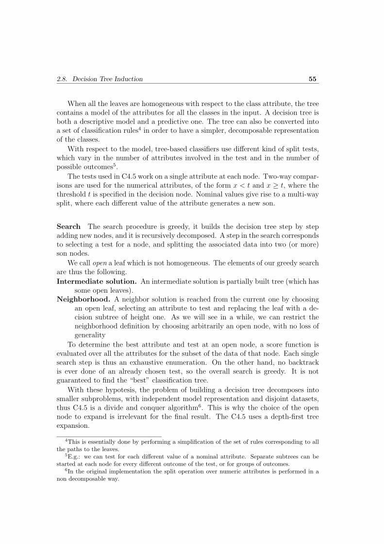
When all the leaves are homogeneous with respect to the class attribute, the treecontains a model of the attributes for all the classes in the input. A decision tree isboth a descriptive model and a predictive one. The tree can also be converted intoa set of classification rules4 in order to have a simpler, decomposable representationof the classes.

With respect to the model, tree-based classifiers use different kind of split tests,which vary in the number of attributes involved in the test and in the number ofpossible outcomes5.

The tests used in C4.5 work on a single attribute at each node. Two-way compar-isons are used for the numerical attributes, of the form x < t and x ≥ t, where thethreshold t is specified in the decision node. Nominal values give rise to a multi-waysplit, where each different value of the attribute generates a new son.

Search The search procedure is greedy, it builds the decision tree step by stepadding new nodes, and it is recursively decomposed. A step in the search correspondsto selecting a test for a node, and splitting the associated data into two (or more)son nodes.

We call open a leaf which is not homogeneous. The elements of our greedy searchare thus the following.Intermediate solution. An intermediate solution is partially built tree (which has

some open leaves).Neighborhood. A neighbor solution is reached from the current one by choosing

an open leaf, selecting an attribute to test and replacing the leaf with a de-cision subtree of height one. As we will see in a while, we can restrict theneighborhood definition by choosing arbitrarily an open node, with no loss ofgenerality

To determine the best attribute and test at an open node, a score function isevaluated over all the attributes for the subset of the data of that node. Each singlesearch step is thus an exhaustive enumeration. On the other hand, no backtrackis ever done of an already chosen test, so the overall search is greedy. It is notguaranteed to find the “best” classification tree.

With these hypotesis, the problem of building a decision tree decomposes intosmaller subproblems, with independent model representation and disjoint datasets,thus C4.5 is a divide and conquer algorithm6. This is why the choice of the opennode to expand is irrelevant for the final result. The C4.5 uses a depth-first treeexpansion.

4This is essentially done by performing a simplification of the set of rules corresponding to allthe paths to the leaves.

5E.g.: we can test for each different value of a nominal attribute. Separate subtrees can bestarted at each node for every different outcome of the test, or for groups of outcomes.

6In the original implementation the split operation over numeric attributes is performed in anon decomposable way.


Score Function The score function which guides the choice of the split test isthe gini index, which is a measure of the gain in entropy by splitting with the giventest.

The information gain of the test is computed in term of the entropy of thegenerated partition. We define the entropy of a set S of data with respect to the setCk of classes

info(S) = −k∑

j=1

(freq(Cj, S)

|S| × log2freq(Cj, S)

|S|

)

(2.2)

where freq(Cj, S) is the number of cases with class Cj in the given set S. Informationgain is a combination of the entropy of node T0 to be expanded with that of theresulting partitions Ti. Its definition is

gain(T0, T1 . . . Tb) = info(T0) −b∑

i=1

(|Ti||T0|

× info(Ti)

)

(2.3)

Evaluation of the split on a nominal attribute requires building histograms ofall the couples (attribute value, class). This can be done with a scan of the currentsubset of instances. On the other hand, when evaluating a test on a numericalattribute, the two classes T1 and T2 are defined by a split point t. The computationof the best split point (which gives the lowest value of the score function for thatnode) requires to access the column of each numerical attribute in sorted order.

Data Management In the original formulation of C4.5 [Qui93] data managementissues are not taken into account. Since a great deal of sorting and scan operationshappen on varying subsets of the input, the algorithm is designed to work in-coreand simply use large arrays and index tables to access the data.

Chapter 3

Parallel Data Mining

In this chapter we discuss the advantages and issues of parallel programming for datamining algorithms and systems. While it is rather obvious that parallel computationcan boost the performance of data mining algorithms, it is less clear how parallelismwould be exploited at best. Starting from the decomposition of the algorithmsgiven in chapter 2, we examine the opportunities for parallelism exploitation in thedifferent components.

In section 3.1 we begin our discussion by confronting the issues of parallel anddistributed data mining. There is a growing opportunity of interaction between thetwo approaches, as hierarchical system architectures (SMP clusters and computa-tional grids) become commonplace in HPC.

Section 3.2 is the main part of the chapter. Parallel decomposition of the al-gorithm requires structural changes that can impact several different levels of thealgorithm. We now look at which components of the mining algorithm need tobe changed, what are the parallel design options for each one, and their reciprocalinteractions.

We distinguish the two interdependent classes of data components (section 3.2.1)and functional components (section 3.2.2) in data mining algorithms. The elemen-tary components described in the previous chapter can be seen as more related tothe functional nature of the algorithm (the score function, see section 3.3, and thesearch strategy, section 3.4) or to the organization of its data (section 3.5 is aboutdata management).

Section 3.6 compares our results with related work about common patterns forparallelism exploitation in data mining algorithms. The chapter ends with sec-tion 3.7 about the issues of KDD system integration for parallel data mining algo-rithms.

58 Chapter 3. Parallel Data Mining

3.1 Parallel and Distributed Data Mining

The problem of exploiting parallelism in data mining algorithms (Parallel DataMining, PDM) is closely related to the issues of distributed data mining (DDM).Both research fields aim at the solution of scalability and performance problems fordata mining by means of parallel algorithms, but in different architectural settings.As it generally happens with the fields of parallel and distributed computing, partof the theory is common, but the actual solutions and tools are often different.

PDM essentially deals with parallel systems that are tightly coupled. Amongthe architectures in this class we find shared memory multiprocessors, distributedmemory architectures, clusters of SMP machines, or large clusters with high-speedinterconnection networks.

DDM, on the contrary, concentrates on loosely coupled systems such as clustersof workstations connected by a slow LAN, geographically distributed sites over awide area network, or even computational grid resources.

Both parallel and distributed data mining offer the common advantages thatcome from the removal of sequential architecture bottlenecks. Higher I/O band-width, larger memory and computational power result than those of existing se-quential systems, all these factors leading to lower response times and improvedscalability to larger data sets.

The common drawback is that algorithm and application design becomes morecomplex. We need to devise algorithms and techniques that distribute the I/O andthe computation in parallel, minimizing communication and data transfers to avoidwasting resources.

In this view PDM has its central target in the exploitation of massive and fine-grain parallelism, paying closer attention to synchronization and load balancing, andexploiting high-performance I/O subsystems where available. PDM applicationsdeal with large and hard problems, and they are typically designed for intensivemining of centralized archives.

By contrast, DDM techniques use a coarser computation grain and loose assump-tions on interconnection networks. DDM techniques are often targeted at distributeddatabases, where data transfers are minimized or replaced by moving results in theform of intermediate or final knowledge models. A widespread approach is indepen-dent learning integrated with summarization and meta-learning techniques such asvoting, arbitration and combining. The work [PCS00] is a excellent survey aboutmeta-learning techniques and on other issues of distributed data mining.

Distributed data mining comes into play because our data and computing re-sources are often naturally distributed. Some databases are distributed over severaldifferent sites and cannot be centralized to perform the DM tasks. There may becost reasons for that, because moving huge datasets from several different sites toa centralized repository is a costly and lengthy operation despite broad-band dataconnections. Moreover, moving a whole database can be a security issue if the dataare valuable. Many countries have regulations that restrict from freely transferring

3.2. Parallelism Exploitation in DM Algorithms 59

certain kinds of data, for instance in order to protect personal privacy rights. It maythen even be illegal for a multinational firm to mine its databases in a centralizedfashion. If the data transfer is not a problem, other resources might be. Centralizedmining of the whole data may require too much computational power or storagespace for any of our computing facilities. In this cases, a distributed algorithm isthe only way to go.

The two fields of PDM and DDM are not rigidly separated, however. Dependingon the relative characteristics of the problem and of the computational architecture,the distinction between fine grain, highly synchronized parallelism and coarse grainparallelism may be not too sharp.

Also in view of recent architectural trends, massively parallel architectures andlarge, loosely coupled clusters of sequential workstations can be seen as the extremesof the range of large-scale High-Performance platforms for Computational Grids atthe cluster, Intranet and Internet level [FK98a].

High performance computer architectures are more and more often based on alarge number of commodity processors. Scaling SMP architectures is difficult andcostly, so large clusters of SMPs are becoming increasingly popular resource forparallel computation at high degrees of parallelism. Beside the use of dedicated,fast interconnection networks, the technology of distributed systems and of parallelones is nearly the same. On the other hand, the enhancement of local area networksmakes possible to use distributed computing resources in a more coordinated waythan before. The building of Beowulf-class parallel clusters, the exploitation of theInternet for grid computing or for distributed computing are all expressions of thediminishing gap among massively parallel and distributed computing.

As already noticed in [Zak99] it is thus definitely realistic to devise the feasibilityof geographically distributed data mining algorithms, where the local mining taskis performed by a parallel algorithm, eventually on massively parallel hardware.

3.2 Parallelism Exploitation in DM Algorithms

We want exploit parallelism to remove the processing speed bottleneck, main mem-ory size bottleneck and I/O bandwidth bottleneck of sequential architectures, thussolving the performance and scalability issues of data mining algorithms.

In order to achieve these results, we have to confront with the design of parallelalgorithms, which adds a new dimension to the design space of programs. Mixingthe implementation details of parallelism and data access management with those ofthe search strategy makes the design of a parallel data mining algorithm a complextask.

We have seen in the previous chapter that a data mining algorithm can bespecified in term of five abstract characteristics:

• the data mining task that it solves;


• the knowledge model that the algorithm uses;

• the score function that guides the model search;

• the search strategy employed;

• the data management techniques employed in the algorithm.

In this chapter we look at the possible decomposition of these components, exploringthe options for parallelism exploitation in order to identify problems, and interac-tions among the components. We will also try to separate as much as possiblethe consequences of parallelism exploitation on different levels of the data miningapplication.

Having chosen a specific data mining technique, we can split the algorithm com-ponents in two main classes that obviously interact with each other, the data com-ponents and the functional components. The data components will have to be par-titioned, replicated or distributed in some way in order to decompose their memoryrequirements, and to distribute in parallel the workload due to the functional compo-nents of the algorithm. On the other hand, the functional components will requiremodification in order to be parallelized, leading in general to a parallel overheadwhich depends on the data decomposition and on the characteristics of the originalfunctions.

Our design choices depend on how much effective is the partitioning of data ininducing independent computations, compared to how high is the cost for splittingproblems and recomposing results at the end of the parallel algorithm.

3.2.1 Data Components

Data components are the two main data structures that the algorithm works on,the input and the model representation. We continue to use the tabular view: sincethe meaning and the management of the data are quite different, and have a deepimpact on the parallelization of the functional parts of the algorithm, we will dealwith instances and attributes as different data components, which are decomposedalong two independent axes.

Data decompositions are often found in sequential data mining too, as enforcedby the issues of memory hierarchy management (section 1.6). Thus considering splitsof the input along two directions, we distinguish three main parallelization optionswith respect to the data structures.

Instances The records in the input D usually represent different elements. Hori-zontal partitioning into blocks does not change the meaning of the data items,and it is often simply called data partitioning in the literature. In the followingwe will use both terms to generally mean partitioning the records into subsets,not necessarily in consecutive blocks. Horizontal partitions usually producesmaller instances of the same data mining problem.

3.2. Parallelism Exploitation in DM Algorithms 61

Attributes Separate vertical partitions (subsets of attributes in the input data)represent a projection of the input in a narrower data space. The meaningof data is now changed, as any knowledge resulting from correlation amongattributes belonging to different vertical partitions is disregarded. This maynot be a problem if we want to compute score functions which do not dependon attribute correlation (e.g. attribute statistic properties), or if the separatesub-models can be efficiently exploited to recompose a solution to the originalproblem.

Model Since data mining employs a wide range of different knowledge models, wedo not try to specify in a general way how a model can be partitioned, we justunderline a few issues. One issue is the kind of dependence of the model fromthe data, if all the data concur in specifying each part of the model, or if it ispossible to devise a decomposition of the model which corresponds to one ofthe input set.

Knowledge models consisting of pattern sets are a peculiar issue, as parti-tioning of the pattern space usually induces some easily understandable (butunknown) kind of partitioning on the input data1. This leads to a viciouscircle, since to exploit the data partitioning we need information about themodel structure, which is exactly what we expect to get from the algorithm.Some pattern-mining algorithms thus exploit knowledge gained from samplingto optimize the main search process, or intermediate, partial knowledge gainedso far to optimize data placement for the following steps.

While we have been talking about partitioning, in some cases we can exploit instead(partial) replication of data, attributes or model components. There is an additionaltradeoff involving how much parallelism we can introduce, how much informationwe replicate, and the overhead of additional computation to synchronize or mergethe different copies.

A main choice about data components is if data partitioning has to be staticor dynamic. The tradeoff here is among data access time at run time and paralleloverhead in the functional components due to the additional computation and datamanagement.

Example 3.1 The induction of decision trees from numeric values described in sec-tion 2.8 is an example of a difficult choice among static and dynamic partitioning.Using the gini index score function leads to a vertical access pattern to the datacolumns in sorted order, while the underlying knowledge model requires horizontal,unbalanced partitioning of the data at each search step. Data partitioning schemesthus need to balance access locality and load balancing. We will discuss the problemin chapter 6.

1The projection of a partitioning in the pattern space is often a set of subsets in the data, nota real data partition. An example is found in association rule mining, described in chapter 5.


3.2.2 Functional Components

Functional Components operate on the data, so their parallelization is linked to thatof the data components. Functional decomposition implies a parallel overhead thatcan sometimes be negligible, but can also dominate the computational cost.

Score Function The score function we use to evaluate a model or a sub-model overthe data can exhibit several properties which can ease some of the decompo-sition strategies. A first issue is that score functions may have a prevalenthorizontal or vertical access pattern to the data, according to their instance-oriented or attribute-oriented nature. Functions with unordered access pat-terns can exploit different data structures to reorganize the data. Score func-tions defined on large arrays can lead to data-parallel formulation, if the loadbalancing and synchronization issues can be properly addressed.

Search Strategy Depending on the kind of search strategy employed, several par-allelism opportunities can be considered

• sub-model parallelism

• state space parallelism

• search-step level parallelism

Sub-model parallelism means splitting the model in several independentsub-models, where separate searches can aim for the locally best sub-model.The results are then composed into a solution for the larger problem. Thestate space is partitioned in this case.

State-space parallelism in our view is running in parallel several searchesin parallel in the same state space.

Search step parallelism is exploited by evaluating in parallel several candi-dates for the next step, to select the best one. It essentially requires exploitingparallelism among more invocations of the evaluation function within a neigh-borhood of the current solution.

The parallel decomposition of the search process interacts with the knowledgemodel decomposition. Another issue for the search strategy is exploiting staticor dynamic partitioning of the model and the state space.

Other data management tasks Data management tasks may be inherited by thesequential formulation of the algorithm (DBMS-resident or disk-resident data,complex data structures like external memory spatial indexes). However, thehardest management tasks for parallel algorithms often come from the choicesmade in partitioning the data to exploit parallelism. An example can bethe need to reorganize the data when employing dynamic partitioning of thedataset. It is a significant cost in the computation, which has to be balancedwith the saving in exploiting a higher degree of locality.

3.3. Parallelism and Score Functions 63

For each functional component at least three cases are possible with respect tothe overhead of parallel decomposition.

• The overhead can be inexistent, because the operations performed are actuallyindependent.

• The overhead is low, it is due to simple summarization operations, whichproduce aggregate results, and/or to broadcast communications, which spreadthe parameters of the current model. Here we assume that the computationand the communication volume are negligible, but we must keep into accountthe need to synchronize different execution units in order to exchange the data.Load balancing, for instance, is an issue in this case.

• We can have a moderate overhead in decomposing a part of the algorithm.For instance, we have to join different parts of the model, or to access datathat is not local, which results in additional computation with respect to thesequential case. The overhead will influence the speed-up and scalability ofthe algorithm, but the parallelization may still be effective.

• In the worst case, the amount of work needed to split the computation iscomparable to the computation itself, so there is no easy way to parallelizethis function. An example is the need to sort data for the sake of tree induction,which accounts for the largest part of the computational cost of the algorithm(see chapter 6). We can apply the best possible techniques. It may also bepossible to parallelize other components of the algorithm.

The hard issue is that these behaviors are often interdependent among the dif-ferent functional components, either directly or because of the decomposition of thedata structures.

3.3 Parallelism and Score Functions

Computing in parallel the score function that evaluates our model over the inputset is the first and easy way to exploit parallelism in a data mining algorithm. If thecomputation of the score function over the whole input can be decomposed to exploitdata parallelism, we can increase the speedup and scalability of the algorithm. Thelimiting assumptions are that the computation involves all the data set and theparallel overhead (the cost of communicating and composing the partial results) isbounded.

Several problems from optimization theory have been confronted this way [CZ97].The data and the model in this case are expressed by matrices, and evaluation ofthe current solution is defined by algebraic operations on rows and blocks of data.


The formalization of the problems leads easily to the exploitation of FORTRAN-like data parallel programming models, where parallelism is essentially expressedby distributing large arrays and applying the owner-compute rule.

Most of the efforts in the field are put in developing decomposition of the scorefunction, and of the algorithm, that make efficient use of this formalism. The maindifficulties are achieving efficient operation on sparse matrices, and computationalworkload balancing.

Data parallel evaluation functions can be exploited in some data mining prob-lems, but the general framework is different from numerical optimization. In op-timization theory we want to find a good solution to a hard problem, thus weuse algorithms that spend a large number of iterations in improving a solution.Exponential-complexity problems are common, and improved solutions are oftenvaluable, so performance and algorithmic gains aim at finding better solutions andmaking larger problem instances computationally tractable. The parallel design ef-fort is put in achieving near peak performance on in-memory (eventually sharedmemory) computation.

While we find worst-case exponential problems in data mining too, the simplesize of the data restrain us from using sophisticate algorithms, and we have to settlefor simpler algorithms. It is much less likely that the data can fit in memory, sosecondary memory issues have to be taken into account even when the data is fullydistributed across the machine. We more often aim at distributing the data and atkeeping low the number of iterations, because the simple cost of out-of-core dataaccess can easily dominate the algorithm behavior.

Example 3.2 An algorithm of the former kind is the EMax (expectation maximiza-tion) method employed in several numerical optimization problems, like in 3D im-age reconstruction [CZ97], and also in the Autoclass algorithm of section 2.7. Theamount of computation required by Autoclass is quite high, and the score function isessentially data parallel, so it is impractical to execute it on out-of core datasets.

Data parallel schemes like those discussed in [BT02] allow to decompose the scorefunction computation, and to execute the algorithm on larger datasets, at the expenseof a certain communication overhead.

Generic score functions that are not easily implemented as data parallel, maystill be usefully decomposable into sub-functions that can be computed on subsetsof the input.

Example 3.3 Functions that compute statistics about the value of a small set ofattributes are well suited to vertical partitioning. As an example, the informationgain used in C4.5 and in other decision tree classifiers (see section 2.8) is computedindependently on each attribute of a data partition. Vertically partitioning the datais a good solution to speed up the computation, but it is difficult to match it with therecursive nature of the search, which implies horizontally splits to generate subprob-lems. The speed-up in the score function by attribute partitioning is furthermore

3.4. Parallelism and Search Strategies 65

limited by the number of the attributes, and by poor load balancing (the columnsrequire different computing resources, and many of them are no longer used as thesearch proceeds to smaller subproblems).

Example 3.4 The score function in association rule mining is the number of oc-currences of a pattern in the database. By using a vertical representation for thedata and for the patterns (which is known as TID-list representation, see chapter 5)the score function for each pattern is the length of its TID-list, which is triviallycomputed when generating the lists during the algorithm.

3.4 Parallelism and Search Strategies

Several different search strategies are employed in data mining algorithm, with someof them being easily parallelizable.

Usually the outermost structure of the search is a loop2, and often more strategiesare mixed or nested inside each other. Two nested levels of search are commonlyfound, which have different characteristics from the point of view of parallelization.Moreover, several of these strategies can be guided by heuristics in order to prunethe space and gain better performance.

We summarize the most commonly employed search strategies.

Local search. This is the general form of all state-space searches which cannot useglobal information about the state space. Local searches move across points inthe state space (the intermediate solutions) by exploiting information abouta neighborhood of the current solution. The neighborhood may be explicitlydefined, or implicitly defined by means of operators which produce all neighborstate representations. Local searches may exploit a different degree of memory,as well as exact or heuristic properties of the problem to improve and speedup the search.

Greedy search. It is an example of a local search which selects the mostpromising point in the neighborhood and never backtracks. While theyexploit all the available information in the neighborhood, greedy methodsin general stop at a local optimum, not at the global optimum.

Branch and bound. It is an example of local search which aims at exploringthe whole state space. It backtracks after finding a local optimum andlooks for unexplored subspaces. Branch and bound implicitly enumerateslarge portions of the state space by exploiting the additive property ofthe cost function to rule out unproductive subspaces.

2In some cases a loop is a simple implementation of a more complex strategy. See for instancethe implementation of the C4.5 algorithm, whose D&C structure is mapped in the sequentialimplementation to a depth-first tree visit. We used a data-flow loop to implement D&C in parallel.


Optimization methods. Several numerical methods exist which exploit analyticproperties of the score function to explore the state space.

Steepest descent. It is the equivalent of greedy local search, as it selects thenext step by following the gradient of the score function at the currentsolution (the most promising direction, which approximatively selects thebest solution in a small neighborhood) and it never explicitly backtracks.In the general case, steepest descent may converge to a local optimum,and is not always granted to converge.

EMax algorithm. The expectation-maximization strategy, briefly describedin section 2.7, iterates alternating the optimization of two different scorefunctions, looking for the best point in the state space which explainsthe input data. As steepest descent, EMax can converge toward a localoptimum.

Randomized techniques. By simply generating a random point in the solutionspace, we can obtain information about that point alone. The dimension of theparameter space prevents from applying purely randomized strategies to datamining. However, randomized strategies are commonly employed to reducethe likelihood that other search strategies get stuck in a local optimum.

Exhaustive search. This kind of search simply tries every combination of param-eters to produce all possible states. Given the size of the input and of thestate space, it is never used alone in data mining problems. It is applied toparticular subproblems (e.g. exploring the neighborhood of a solution).

Collective strategies. We group under this name all search strategies which em-ploy a (possibly large) set of cooperating entities which interact in the processof finding a solution. Examples of collective search are genetic algorithms orant-colony-like optimization methods [CDG99].

From the point of view of parallel execution or decomposition, we must lookat the feasibility of splitting the solution space and partitioning the model. As wementioned before in the chapter, we can exploit

• sub-model parallelism (split state space)

• state space parallelism (shared state space)

• search-step level parallelism. (shared state space, same current solution)

Collective strategies implicitly use a shared model space. However, it has beenobserved that some collective strategies exhibit a “double speed-up” phenomenon,discussed in section 3.6, which makes them well-suited for parallelization.

Randomized strategies also impose no particular problem, as sampling the statespace can easily be done in parallel. However, replication of all the data is required,

3.5. Parallel Management of Data 67

which can be an issue. When used as an outer loop strategy, it may happen that therandomization is guided by the preceding attempts (this is the case of Autoclass,for instance). It may well happen that the results of applying several randomizedsearches independently is not equivalent to running them in sequence. The perfor-mance and the quality of the solution may thus not improve as expected.

It requires analysis of the model to understand if a local search can be exploitedon sub-models. As a general rule, it is easier to build patterns than models this way.It is often the case that the sub-models are induced by a split in the input data (anexample is the effect on the pattern space of association rules by careful partitioningof the input) and are thus not entirely disjoint.

Complex strategies like the EMax one give an edge to the parallelization of theirlower-level tasks, like the computation of the score function.

While we have been discussing the options of parallelization of the search, we havenot yet addressed a key point, the structure of the model. If the model is not flat,i.e. it has a recursive structure, then there are chances that the optimization taskson the parameters of the sub-models can be separated. This happens for differentbranches of decision trees, and in some hierarchical clustering algorithms (this is thecase of CLIQUE [AGGR98]). As we turn sequential sub-model computations intoparallel, we also map a sequential visit of the model structure, which accomplishesthe search in the sequential case, into a parallel expansion scheme.

Example 3.5 For decision trees, the tree expansion schemes (depth first search,breadth first search) tend to be mapped into breadth first expansions which operateon all the nodes of a level in parallel. The actual expansion process is howeverconstrained by other issues, like load balancing, communication and synchronizationcosts. More complex search strategies are thus developed, which modify their behaviorat run time, based on problem and performance measurements.

3.5 Parallel Management of Data

The data management issues are a concern already for sequential data mining algo-rithms. The parallel version of an algorithm inherits these issues (in-memory datamanagement, out-of-core management, DBMS exploitation). Among them, exploit-ing a DBMS for parallel mining is usually the hardest problem, as a single DBMSmay not be able to service the amount of queries generated by a parallel program.

Parallel I/O exploitation is easily realized by means of local resources in eachprocessing node if we know how to partition the data, and if the partitions arebalanced.

There are however other issues that result from partitioning the input data.Splitting the data horizontally or vertically, according to the decomposition of ourmodel and search, may require to reorganize the data before running the algorithm.

Two main problems surface.


• Complex data structures used to optimize data management may not be easilyturned into parallel ones.

• It happens that there is no static partitioning that allows strictly local com-putation, or that such a partitioning cannot be computed in advance.

Example 3.6 Many clustering algorithm, including k-means, can employ tree-likedata structures to keep close points together and exploit memory locality. Clusteringalgorithms avoid useless computation by maintaining clustering features and bound-ing boxes of sets of point to avoid repeated computations. These data structures how-ever are hard to decompose in parallel, as their internal organization changes duringthe algorithm. The same problem is faced in several numerical simulation whichaim at dynamically exploiting the evolving spatial properties of data (e.g. adaptivemultigrid methods).

Note that in the case of k-means clustering, what actually needs data managementis the amount intermediate information that is used to direct the search of our nicelycompact model (the set of centroids).

Example 3.7 In decision tree induction, the subdivision of the initial problem intosubproblems is inherently dynamic and unpredictable. Reorganizing the input dataat each search step (or bookkeeping additional information to allow efficient accessanyway) accounts for the the largest part of the data management task.

3.6 Related Work on Parallelism Exploitation

The analysis of parallel mining algorithm set forth in this chapter is an extension ofthe reductionist viewpoint presented in [HMS01] to take into account the parallelism-related issues.

Some of the work is based on an article by Skillicorn [Ski99] which distinguishesthree classes of data mining algorithms. A high-level cost model is also proposedthere for these classes, which is based on the BSP cost model. We have not yetdeveloped our analysis to produce a cost model of this kind, which is undoubtedlya useful tool in designing algorithms. We believe that extensions of the BSP model,which are capable to deal with hierarchical memory issues (see section 1.6.1), willplay a major role in developing more portable parallel algorithms.

In [Ski99] three classes of parallel mining algorithms are characterized. Allof them are actually generalized to an iterative form of more consecutive parallelphases, which in the following we omit for the sake of conciseness.

Independent search is based on replicated input data and completely indepen-dent searches.

Algorithms in this class exploit the simplest form of parallel search, where allthe input data is replicated and parallel execution of the sequential algorithm

3.6. Related Work on Parallelism Exploitation 69

independently explore the same state-space, which defines the whole model.This class of parallel algorithms is important, as it can be extended to includecomplex algorithms employing randomization as their outer-level search strat-egy (e.g. clustering algorithms like Autoclass and k-means, or multiple-windowsupervised classification approaches).

Parallelized sequential is based on partitioning the input (instances or attributes)and employ the subdivision of the space-state that results in multiple parallelexecutions. The results are then joined to produce the true answer.

The attribute/instance-based partitioning projects the original state space intopossibly smaller spaces for each partition. This is natural when doing verticalpartitioning, as the model loses some of its parameters. In the case of hori-zontal partitioning the projected state space may coincide with the initial one.This class of parallelizations thus contains two subclasses, depending on thekind of join operation needed to reconcile the partial models.

• Models in the same state space need to be confronted to integrate knowl-edge. It is often the case that the resulting model is simply some kindof “sum” of the components which requires a small computational effortand/or a global validation.

• Models belonging to different state spaces usually need a more complexrecomposition operation.

The parallelized algorithm class actually covers a wide range of algorithms,which exhibit a range of different recomposition issues for the knowledge gainedin the parallel part of the computation. Estimating the computational cost ofthe joining phase requires a more in-depth analysis of the data mining algo-rithm. Looking from a different point of view, this class includes algorithmsthat obliviously partition the input and others that try to exploit informedpartitioning scheme to enhance the independence of the resulting paralle com-putations.

Replicated sequential applies an instance-based (horizontal) partitioning to ex-ploit independent sequential search for approximate concepts.

This could be actually seen as a subclass of the Parallelized-sequential one,but we use the specific assumption that the kind of model allows to generatecomplete models from horizontal partitions, and that these partial answersare all approximations of the final one. We assume that they can be joinedwith a relatively simple algorithm, and then verified or integrated in parallelover the data partitions. Algorithms in this class tend to parallelize well, asthe parallel overhead is fairly bounded. Some of them also enjoy the benefitof a “double speedup” phenomenon. The exchange at each phase of highly


concentrated knowledge3 allows each independent search to quickly convergein the state space, like if it had available a much larger amount of data thanits own partition.

3.7 Integration Issues

It is now recognized that a crucial issue in the effectiveness of DM tools is the degreeof interoperability with conventional databases, data warehouses and OLAP services.Maniatty and Zaki [MZ00] state several requirements for parallel DM systems, andthe issues related to the integration are clearly underlined.

System Transparency is the ability to easily exploit file system access as wellas databases and data warehouses. This feature is not only a requirement of toolinteroperability, but also an option to exploit the best software support available indifferent situations.

Most mining algorithms, especially the parallel ones, are designed for flat-filemining (exploiting data-mining on flat files with an algorithm-specific layout). Thissimplification eases initial code development, and it is often justified by the access toDBMS being too slow for high-performance computation. On the other hand, beingrestricted to flat-file mining imposes an overhead when working with higher-leveldata management supports (e.g. we need to dump the data to a specific format andto fully materialize DBMS views).

Industry standards are being developed to address this issue in the sequentialsettings, as noted in section 2.4, and research is ongoing about the parallel case (seefor instance the book by Freitas and Lavington [FL98]). We can distinguish threemain approaches.

• Development of data mining algorithms based on existing standard interfaces(e.g. SQL). Many algorithms have been rewritten or designed to work bymeans of DBMS primitives. DBSCAN (chapter 7) is designed assuming theuse of a spatial database system.

• Development of a few new database-mining primitives within the frame ofstandard DBMS languages (a crucial issue is the expressive power that wemay gain or lose).

• Design of dedicated, possibly parallel mining interfaces to allow tight integra-tion of the mining process with the data management.

Pushing more of the computational effort into the data management supportmeans exploiting the internal parallelism of modern database servers. On the otherhand, scalability of such servers to massive parallelism is still a matter of research.

3Here we view each knowledge searching process as trying to compress information about itsdata partition.

3.7. Integration Issues 71

While integration solutions are now emerging for sequential DM, this is not the casefor parallel algorithms yet.

The bandwidth of I/O subsystems in parallel architectures is theoretically muchhigher than that of sequential ones, but a conventional file system or DBMS interfacecannot easily exploit it. We need to use new software supports that are still far frombeing standards, and sometimes are architecture-specific.

Parallel file systems, high performance interfaces to parallel database serversare important resources to exploit for PDM. DDM must also take into accountremote data servers, data transport layers, computational Grid resources, and allthe issues about security, availability, and fault tolerance that are commonplace forlarge distributed systems.

Our approach is to develop a parallel programming environment that addressesthe problem of parallelism exploitation within algorithms, while offering uniforminterfacing characteristics with respect to different software and hardware resourcesfor data management. Structured parallelism will be used to express the algorith-mic parallelism, while an object-like interface will allow accessing a number of usefulservices in a portable way, including other applications and CORBA-operated soft-ware.


Documents

Chapter 2 Knowledge Discovery and Data Mining