Chapter 2- Isodual Theory of Point-Like Antiparticles

8/3/2019 Chapter 2- Isodual Theory of Point-Like Antiparticles

http://slidepdf.com/reader/full/chapter-2-isodual-theory-of-point-like-antiparticles 1/50

Chapter 2

ISODUAL THEORY OF

POINT-LIKE ANTIPARTICLES

2.1 ELEMENTS OF ISODUAL MATHEMATICS

2.1.1 Isodual Unit, Isodual Numbers andIsodual Fields

The first comorehensive study of the isodual theory for point-like antipar-ticles has been presented by the author in monograph [34]. However, thefield is subjected to continuous developments following its first presentation inpapers [1] of 1985. Hence, it is important to review the most recent formula-tion of the isodual mathematics in sufficient details to render this monographselfsufficient.

In this section, we identify only those aspects of isodual mathematics thatare essential for the understanding of the physical profiles presented in thesubsequent sections of this chapter. We begin with a study of the most funda-mental elements of all mathematical and physical formulations, units, numbersand fields, from which all remaining formulations can be uniquely and unam-biguously derived via simple compatibility arguments. To avoid un-necessaryrepetitions, we assume the reader has a knowledge of the basic mathematicsused for the classical and operator treatment of matter.

DEFINITION 2.1.1: Let F = F (a, +, ×) be a field (of characteristic zero),namely a ring with elements given by real number a = n, F = R(n, +, ×),complex numbers A = c, F = C (c, +, ×), or quaternionic numbers a = q, F =

Q(q, +, ×), with conventional sum a + b verifying the commutative law

a + b = b + a = c ∈ F, (2.1.1)

the associative law

(a + b) + c = a + (b + c) = d ∈ F, (2.1.2)



96

conventional product a × b verifying the associative law

(a × b) × c = a × (b × c) = e ∈ F, (2.1.3)

(but not necessarily the commutative law, a × b = b × a since the latter isviolated by quaternions), and the right and left distributive laws

(a + b) × c = a × c + b × c = f ∈ F, (2.1.4a)

a × (b + c) = a × b + a × c = g ∈ F, (2.1.4b)

left and right additive unit 0,

a + 0 = 0 + a = a ∈ F, (2.1.5)

and left and right multiplicative unit I ,

a × I = I × a = a ∈ F, (2.1.6)

∀a,b,c ∈ F . Santilli’s isodual fields (first introduced in Refs. [1] and then presented in details in Ref. [2]) are rings F d = F d(ad, +d, ×d) with elementsgiven by isodual numbers

ad = −a†, ad ∈ F, (2.1.7)

with associative and commutative isodual sum

ad +d bd = −(a + b)† = cd ∈ F d, (2.1.8)

associative and distributive isodual product

ad ×d bd = ad × (I d)−1 × bd = cd ∈ F d, (2.1.9)

additive isodual unit 0d = 0,

ad +d 0d = 0d +d ad = ad, (2.1.10)

and multiplicative isodual unit I d = −I †,

ad ×d I d = I d ×d ad = ad, ∀ad, bd ∈ F d. (2.1.11)

The proof of the following property is elementary.

LEMMA 2.1.1 [1,2]: Isodual fields are fields, namely, if F is a field, itsimage F d under the isodual map is also a field.



ELEMENTS OF HADRONIC MECHANICS, VOL. III 97

The above lemma establishes the property (first identified in Refs. [1]) thatthe axioms of a field do not require that the multiplicative unit be necessarily positive-definite, because the same axioms are also verified by negative-definiteunits. The proof of the following property is equally simple.

LEMMA 2.1.2 [1,2]: Fields F and their isodual images F d are anti-iso-morphic to each other.

Lemmas 2.1.1 and 1.2.2 illustrate the origin of the name “isodual mathe-matics”. In fact, to represent antimatter the needed mathematics must be asuitable “dual” of conventional mathematics, while the prefix “iso” is used inits Greek meaning of preserving the original axioms.

It is evident that for real numbers we have

nd = −n, (2.1.12)

while for complex numbers we have

cd = (n1 + i × n2)d = −n1 + i × n2 = −c, (2.1.13)

with a similar formulation for quaternions.It is also evident that, for consistency, all operations on numbers must be

subjected to isoduality when dealing with isodual numbers. This implies: theisodual powers

(ad)nd

= ad ×d ad ×d ad... (2.1.14)

(n times, with n an integer); the isodual square root

ad(1/2)d

= −

−a††, ad

(1/2)d×d ad

(1/2)d= ad, 1d

(1/2)d= −i; (2.1.15)

the isodual quotient

ad/dbd = −(a†/b†) = cd, bd ×d cd = ad; (2.1.16)

etc.An important property for the characterization of antimatter is the follow-

ing:

LEMMA 2.1.3. [2]: isodual fields have a negative–definite norm, called isodual norm,

|ad

|

d =|a†

| ×I d =

−(aa†)1/2 < 0, (2.1.17)

where |...| denotes the conventional norm.

For isodual real numbers we therefore have the isodual isonorm

|nd|d = −|n| < 0, (2.1.18)



98

and for isodual complex numbers we have

|cd|d = −|c| = −(cc)1/2 = −(n21 + n22)1/2. (2.1.19)

LEMMA 2.1.4 [2]: All quantities that are positive–definite when referred to positive units and related fields of matter (such as mass, energy, angular momentum, density, temperature, time, etc.) became negative–definite when referred to isodual units and related isodual fields of antimatter.

As recalled Chapter 1, antiparticles have been discovered in the negati-ve-energy solutions of Dirac’s equation and they were originally thought toevolve backward in time (Stueckelberg, Feynman, and others, see Refs. [1,2] of Chapter 1). The possibility of representing antiparticles via isodual methods

is therefore visible already from these introductory notions.The main novelty is that the conventional treatment of negative–definite

energy and time was (and still is) referred to the conventional unit +1. Thisleads to a number of contradictions in the physical behavior of antiparticles.

By comparison, negative-definite physical quantities of isodual theories arereferred to a negative–definite unit I d < 0. This implies a mathematical andphysical equivalence between positive–definite quantities referred to positive– definite units, characterizing matter, and negative–definite quantities referred to negative–definite units, characterizing antimatter . These foundations thenpermit a novel characterization of antimatter beginning at the Newtonian level,and then persisting at all subsequent levels.

DEFINITION 2.1.2 [2]: A quantity is called isoselfdual when it coincideswith its isodual.

It is easy to verify that the imaginary unit is isoselfdual because

id = −i† = −i = −(−i) = i. (2.1.20)

This property permits a better understanding of the isoduality of complexnumbers that can be written explicitly

cd = (n1 + i × n2)d = nd1 + id ×d nd2 = −n1 + i × n2 = −c. (2.1.21)

The above property will be important to prove the equivalence of isodualityand charge conjugation at the operator level.

As we shall see, isoselfduality is a new fundamental view of nature withdeep physical implications, not only in classical and quantum mechanics butalso in cosmology. For instance we shall see that Dirac’s gamma matrices areisoselfdual, thus implying a basically new interpretation of this equation that




has remained unidentified for about one century. We shall also see that, whenapplied to cosmology, isoselfduality implies equal distribution of matter andantimatter in the universe, with identically null total physical characteristic,such as identically null total time, identically null total mass, etc.

We assume the reader is aware of the emergence here of new numbers, thosewith a negative unit, that have no connection with ordinary negative numbersand are the true foundations of the isodual theory of antimatter.

2.1.2 Isodual Functional Analysis

All conventional and special functions and transforms, as well as functionalanalysis at large, must be subjected to isoduality for consistent applications,resulting in the simple, yet unique and significant isodual functional analysis,studied by Kadeisvili [3], Santilli [4] and others.

We here mention the isodual trigonometric functions

sind θd = − sin(−θ), cosd θd = − cos(−θ), (2.1.22)

with related basic property

cosd 2d θd +d sind 2d θd = 1d = −1, (2.1.23)

the isodual hyperbolic functions

sinhd wd = − sinh(−w), coshd wd = − cosh(−w), (2.1.24)

with related basic property

coshd 2d wd −d sinhd 2d wd = 1d = −1, (2.1.25)

the isodual logarithm and the isodual exponentiation defined respectively by

logd nd = − log(−n), (2.1.26a)

eXdd

= 1d + X d/d1!d + X d2d

/d2!d + ... = −eX , (2.1.26b)

etc. Interested readers can then easily construct the isodual image of specialfunctions, transforms, distributions, etc.

2.1.3 Isodual Differential and Integral Calculus

Contrary to a rather popular belief, the differential calculus is indeed depen-dent on the assumed unit. This property is not so transparent in the conven-

tional formulation because the basic unit is the trivial number +1. However,the dependence of the unit emerges rather forcefully under its generalization.

The isodual differential calculus, first introduced by Santilli in Ref. [5a], ischaracterized by the isodual differentials

ddxk = I d × dxk = −dxk, ddxk = −dxk, (2.1.27)



100

with corresponding isodual derivatives

∂ d/d∂ dxk = −∂/∂xk, ∂ d/d∂ dxk = −∂/∂x, (2.1.28)

and related isodual properties.Note that conventional differentials are isoselfdual , i.e.,

(dxk)d = ddxkd ≡ d xk, (2.1.29)

but derivatives are not isoselfdual ,

[∂f/∂xk]d = −∂ df d/d∂ dxkd. (2.1.30)

The above properties explain why the isodual differential calculus remainedundiscovered for centuries.

Other notions, such as the isodual integral calculus, can be easily derivedand shall be assumed as known hereon.

2.1.4 Lie-Santilli Isodual Theory

Let L be an n–dimensional Lie algebra in its regular representation withuniversal enveloping associative algebra ξ(L), [ξ(L)]− ≈ L, n-dimensional unitI = Diag.(1, 1,..., 1), ordered set of Hermitean generators X = X † ={X k}, k = 1, 2,...,n, conventional associative product X i × X j , and familiarLie’s Theorems over a field F (a, +, ×).

The Lie-Santilli isodual theory was first submitted in Ref. [1] and thenstudied in Refs. [4-7] as well as by other authors [23-31]. The isodual univer-sal associative algebra [ξ(L)]d is characterized by the isodual unit I d, isodual generators X d = −X , and isodual associative product

X di ×d X d j = −X i × X j , (2.1.31)

with corresponding infinite–dimensional basis characterized by the Poincare– Birkhoff–Witt-Santilli isodual theorem

I d, X di ×d X d j , i ≤ j; X di ×d X d j × X dk , i ≤ j ≤ k,... (2.1.32)

and related isodual exponentiation of a generic quantity Ad

edAd

= I d + Ad/d1!d + Ad ×d Ad/d2!d + ... = −eA†

, (2.1.33)

where e is the conventional exponentiation.The attached Lie-Santilli isodual algebra Ld ≈ (ξd)− over the isodual field

F d(ad, +d, ×d) is characterized by the isodual commutators [1]

[X di ,d X d j ] = −[X i, X j ] = C kd

ij ×d X dk . (2.1.34)




with classical realizations given in Section 2.2.6.Let G be a conventional, connected, n–dimensional Lie transformation group

on a metric (or pseudo-metric) space S (x, g, F ) admitting L as the Lie alge-bra in the neighborhood of the identity, with generators X k and parametersw = {wk}.

The Lie-Santilli isodual transformation group Gd admitting the isodual Liealgebra Ld in the neighborhood of the isodual identity I d is the n–dimensionalgroup with generators X d = {−X k} and parameters wd = {−wk} over theisodual field F d with generic element [1]

U d(wd) = edid×dwd×dXd

= −ei×(−w)×X = −U (−w). (2.1.35)

The isodual symmetries are then defined accordingly via the use of the isod-ual groups Gd and they are anti–isomorphic to the corresponding conventionalsymmetries, as desired. For additional details, one may consult Ref. [4,5b].

In this chapter we shall therefore use the conventional Poincare, internal and other symmetries for the characterization of matter , and the Poincare-Santilli, internal and other isodual symmetries for the characterization of an-timatter .

2.1.5 Isodual Euclidean Geometry

Conventional (vector and) metric spaces are defined over conventional fields.It is evident that the isoduality of fields requires, for consistency, a correspond-ing isoduality of (vector and) metric spaces. The need for the isodualities of all quantities acting on a metric space (e.g., conventional and special functions

and transforms, differential calculus, etc.) becomes then evident.

DEFINITION 2.1.3: Let S = S (x,g ,R) be a conventional N -dimen-sional metric or pseudo-metric space with local coordinates x = {xk}, k =1, 2,...,N , nowhere degenerate, sufficiently smooth, real–valued and symmetricmetric g(x,...) and related invariant

x2 = (xi × gij × x j) × I, (2.1.36)

over the reals R. The isodual spaces, first introduced in Ref. [1] (see also Refs.[4,5] and, for a more recent account, Ref. [22]), are the spaces S d(xd, gd, Rd)with isodual coordinates xd = xd = −xt (where t stands for transposed),isodual metric

gd(xd,...) = −g†(−x†,...) = −g(−xt,...), (2.1.37)

and isodual interval

(x − y)d2 d

= [(x − y)id ×d gdij ×d (x − y) jd ] × I d =



102

= [(x − y)i × gdij × (x − y) j] × I d, (2.1.38)

defined over the isodual field Rd = Rd(nd, +d, ×d) with the same isodual isounit I d.

The basic nonrelativistic space of our analysis is the three–dimensional iso-dual Euclidean space [1,9],

E d(rd, δd, Rd) : rd = {rkd} = {−rk} = {−x, −y, −z}, (2.1.39a)

δd = −δ = diag.(−1, −1, −1),

I d = −I = Diag.(−1, −1, −1). (2.1.39b)

The isodual Euclidean geometry is the geometry of the isodual space E d

over Rd and it is given by a step–by–step isoduality of all the various aspects

of the conventional geometry (see monograph [5a] for details).By recalling that the norm on Rd is negative–definite, the isodual distanceamong two points on an isodual line is also negative definite and it is given by

Dd = D × I d = −D, (2.1.40)

where D is the conventional distance. Similar isodualities apply to all remain-ing notions, including the notions of parallel and intersecting isodual lines, theEuclidean axioms, etc.

The isodual sphere with radius Rd = −R is the perfect sphere on E d overRd and, as such, it has negative radius (Figure 2.1),

Rd2d = (xd2d + yd2d + zd2d) × I d =

= (x2 + y2 + z2) × I = R2. (2.1.41)

Note that the above expression coincides with that for the conventionalsphere. This illustrates the reasons, following about one century of studies,the isodual rotational group and symmetry where identified for the first timein Refs. [1]. Note, however, that the latter result required the prior discoveryof new numbers, those with a negative unit.

A similar characterization holds for other isodual shapes characterizing an-timatter in our isodual theory.

LEMMA 2.1.5: The isodual Euclidean geometry on E d over Rd is anti– isomorphic to the conventional geometry on E over R.

The group of isometries of E d over Rd is the isodual Euclidean group E d(3) =Rd(θd) ×d T d(3) where Rd(θ) is the isodual group of rotations first introducedin Ref. [1], and T (3) is the isodual group of translations (see also Ref. [5a] fordetails).




2.1.6 Isodual Minkowskian Geometry

Let M (x,η,R) be the conventional Minkowski spacetime with local coordi-nates x = (rk, t) = (xµ), k = 1, 2, 3, µ = 1, 2, 3, 4, metric η = Diag.(1, 1, 1, −1)and basic unit I = Diag.(1, 1, 1, 1) on the reals R = R(n, +, ×).

The Minkowski-Santilli isodual spacetime, first introduced in Ref. [7] andstudied in details in Ref. [8], is given by

M d(xd, ηd, Rd) : xd = {xµd} = {xµ × I d} = {−r, −cot} × I, (2.1.42)

with isodual metric and isodual unit

ηd = −η = diag.(−1, −1, −1, +1), (2.1.43a)

I d = Diag.(−1, −1, −1, −1). (2.1.43b)

The Minkowski-Santilli isodual geometry [8] is the geometry of isodual spacesM d over Rd. The new geometry is also characterized by a simple isodualityof the conventional Minkowskian geometry as studied in details in memoir.

The fundamental symmetry of this chapter is given by the group of isome-tries of M d over Rd, namely, the Poincare-Santilli isodual symmetry [7,8]

P d(3.1) = Ld(3.1) × T d(3.1) (2.1.44)

where Ld(3.1) is the Lorentz-Santilli isodual group and T d(3.1) is the isodualgroup of translations.

2.1.7 Isodual Riemannian Geometry

Consider a Riemannian space (x,g ,R) in (3+1) dimensions [32] with basicunit I = Diag.(1, 1, 1, 1), nowhere singular and symmetric metric g(x) andrelated Riemannian geometry in local formulation (see, e.g., Ref. [27]).

The Riemannian-Santilli isodual spaces (first introduced in Ref. [11]) aregiven by

d(xd, gd, Rd) : xd = {−xµ},

gd = −g(x), g ∈ (x,g ,R),

I d = Diag.(−1, −1, −1, −1) (2.1.45)

with intervalx2d = [xdt ×d gd(xd) ×d xd] × I d =

= [xt × gd(xd) × x] × I d ∈ Rd, (2.1.46)

where t stands for transposed.The Riemannian-Santilli isodual geometry [8] is the geometry of spaces d

over Rd, and it is also given by step–by–step isodualities of the conventional



104

Figure 2.1. A schematic view of the isodual sphere on isodual Euclidean spaces over isodualfields. The understanding of the content of this chapter requires the knowledge that theisodual sphere and the conventional sphere coincide when inspected by an observer either inthe Euclidean or in the isodual Euclidean space, due to the identity of the related expressions(2.1.36) and (2.1.38). This identity is at the foundation of the perception that antiparticles“appear” to exist in our space, while in reality they belong to a structurally different spacecoexisting within our own, thus setting the foundations of a “multidimensional universe”coexisting in the same space of our sensory perception. The reader should keep in mind thatthe isodual sphere is the idealization of the shape of an antiparticle used in this monograph.

geometry, including, most importantly, the isoduality of the differential andexterior calculus.

As an example, an isodual vector field X d(xd) on d is given by X d(xd) =−X t(−xt). The isodual exterior differential of X d(xd) is given by

DdX kd(xd) = ddX kd(xd) + Γdik j ×d X id ×d ddx jd = DX k(−x), (2.1.47)

where the Γd’s are the components of the isodual connection . The isodual covariant derivative is then given by

X id(xd)|dk = ∂ dX id(xd)/d∂ dxkd + Γdi jk ×d X jd(xd) = −X i(−x)|k . (2.1.48)

The interested reader can then easily derive the isoduality of the remainingnotions of the conventional geometry.

It is an instructive exercise for the interested reader to work out in detail

the proof of the following:

LEMMA 2.1.6 [8]: The isodual image of a Riemannian space d(xd, gd, Rd)is characterized by the following maps:

Basic Unit




I → I d = −I,

Metric

g → gd = −g, (2.1.49a)

Connection Coeff icients

Γklh → Γdklh = −Γklh, (2.1.49b)

Curvature T ensor

Rlijk → Rdlijk = −Rlijk, (2.1.49c)

Ricci T ensor

Rµν → Rdµν = −Rµν , (2.1.49d)

Ricci Scalar

R → Rd = R, (2.1.49e)

Einstein − Hilbert T ensor

Gµν → Gdµν = −Gµν , (2.1.49f )

Electromagnetic P otentials

Aµ → Adµ = −Aµ, (2.1.49g)

Electromagnetic F ield

F µν → F dµν = −F µν , (2.1.49h)

ElmEnergy − Momentum T ensorT µν → T dµν = −T µν , (2.1.49i)

In summary, the geometries significant for this study are: the conventional Euclidean, Minkowskian and Riemannian geometries used for the character-ization of matter ; and the isodual Euclidean, Minkowskian and Riemannian geometries used for the characterization of antimatter .

The reader can now begin to see the achievement of axiomatic compatibil-ity between gravitation and electroweak interactions that is permitted by theisodual theory of antimatter. In fact, the latter is treated via negative-definiteenergy-momentum tensors, thus being compatible with the negative-energysolutions of electroweak interactions, therefore setting correct axiomatic foun-

dations for a true grand unification studied in the next chapter.



106

2.2 CLASSICAL ISODUAL THEORY OF

POINT-LIKE ANTIPARTICLES2.2.1 Basic Assumptions

Thanks to the preceding study of isodual mathematics, we are now suffi-ciently equipped to resolve the scientific impasse caused by the absence of aclassical theory of antimatter studied in Section 1.1.

As it is well known, the contemporary treatment of matter is characterizedby conventional mathematics, here referred to ordinary numbers, fields, spaces,etc. with positive units and norms, thus having positive characteristics of mass,energy, time, etc.

In this chapter we study the characterization of antimatter via isodual num-bers, fields, spaces, etc., thus having negative–definite units and norms. Inparticular, all characteristics of matter (and not only charge) change sign forantimatter when represented via isoduality.

The above characterization of antimatter evidently provides the correct conjugation of the charge at the desired classical level. However, by no means, thesole change of the sign of the charge is sufficient to ensure a consistent classicalrepresentation of antimatter. To achieve consistency, the theory must resolvethe main problematic aspect of current classical treatments, the fact that theiroperator image is not the correct charge conjugate state (Section 2.1).

The above problematic aspect is indeed resolved by the isodual theory. Themain reason is that, jointly with the conjugation of the charge, isodualityalso conjugates all other physical characteristics of matter. This implies twochannels of quantization, the conventional one for matter and a new isodual

quantization for antimatter (see Section 2.3) in such a way that its operatorimage is indeed the charge conjugate of that of matter.In this section, we study the physical consistency of the theory in its classical

formulation. The novel isodual quantization, the equivalence of isoduality andcharge conjugation and related operator issues are studied in the next section.

Beginning our analysis, we note that the isodual theory of antimatter re-solves the traditional obstacles against negative energies and masses. In fact,particles with negative energies and masses measured with negative units are fully equivalent to particles with positive energies and masses measured with positive units. This result has permitted the elimination of sole use of sec-ond quantization for the characterization of antiparticles because antimatterbecomes treatable at all levels, including second quantization.

The isodual theory of antimatter also resolves the additional, well known,problematic aspects of motion backward in time. In fact, time moving back-ward measured with a negative unit is fully equivalent on grounds of causality to time moving forward measured with a positive unit .




This confirms the plausibility of the first conception of antiparticles byStueckelberg and others as moving backward in time (see the historical anal-ysis in Ref. [1] of Chapter 1), and creates new possibilities for the ongoingresearch on the so-called “spacetime machine” studied in Chapter 5.

In this section, we construct the classical isodual theory of antimatter at theNewtonian, Lagrangian, Hamiltonian, Galilean, relativistic and gravitationallevels; we prove its axiomatic consistency; and we verify its compatibility withavailable classical experimental evidence (that dealing with electromagneticinteractions only). Operator formulations and their experimental verificationswill be studied in the next section.

2.2.2 Need for Isoduality to Represent All TimeDirections

It is popularly believed that time has only two directions, the celebrated Ed-dington’s time arrows. In reality, time has four different directions dependingon whether motion is forward or backward and occurs in the future or in thepast, as illustrated in Figure 2.2. In turn, the correct use of all four differentdirections of time is mandatory, for instance, in serious studies of bifurcations,as we shall see.

It is evident that theoretical physics of the 20-th century could not explainall four directions of time, since it possessed only one conjugation, time re-versal, and this explains the reason the two remaining directions of time wereignored.

It is equally evident that isoduality does indeed permit the representationof the two missing directions of time, thus illustrating its need.

We assume the reader is now familiar with the differences between timereversal and isoduality. Time reversal changes the direction of time whilekeeping the underlying space and units unchanged, while isoduality changesthe direction of time while mapping the underlying space and units into dif-ferent forms.

Unless otherwise specified, through the rest of this volume time t will beindicate motion forward toward in future times, −t will indicate motion back-ward in past times, td will indicate motion backward from future times, and−td will indicate motion forward from past times.

2.2.3 Experimental Verification of the Isodual Theoryof Antimatter in Classical Physics

The experimental verification of the isodual theory of antimatter at the clas-sical level is provided by the compliance of the theory with the only availableexperimental data, those on Coulomb interactions.



108

Figure 2.2. A schematic view of the “four different directions of time”, depending onwhether motion is forward or backward and occurs in the future or in the past. Due tothe sole existence of one time conjugation, time reversal, the theoretical physics of the 20-thcentury missed two of the four directions of time, resulting in fundamental insufficienciesranging from the lack of a deeper understanding of antiparticles to basic insufficiencies in

biological structures and excessively insufficient cosmological views. It is evident that isod-uality can indeed represent the two missing time arrows and this illustrates a basic need forthe isodual theory.

For that purpose, let us consider the Coulomb interactions under the cus-tomary notation that positive (negative) forces represent repulsion (attraction)when formulated in conventional Euclidean space.

Under such an assumption, the repulsive Coulomb force among two particlesof negative charges −q1 and −q2 in Euclidean space E (r,δ,R) is given by

F = K × (−q1) × (−q2)/r × r > 0, (2.2.1)

where K is a positive constant whose explicit value (here irrelevant) depends

on the selected units, the operations of multiplication × and division / are theconventional ones of the underlying field R(n, +, ×).

Under isoduality to E d(rd, δd, Rd) the above law is mapped into the form

F d = K d ×d (−q1)d ×d (−q2)d/drd ×d rd = −F < 0, (2.2.2)

where ×d = −× and /d = −/ are the isodual operations of the underlyingfield Rd(nd, +, ×d).

But the isodual force F d = −F occurs in the isodual Euclidean spaceand it is, therefore, defined with respect to the unit −1. This implies thatthe reversal of the sign of a repulsive force measured with a negative unit alsodescribes repulsion. As a result, isoduality correctly represents the repulsivecharacter of the Coulomb force for two antiparticles with positive charges, aresult first achieved in Ref. [9].

The formulation of the cases of two particles with positive charges and theirantiparticles with negative charges is left to the interested reader.

The Coulomb force between a particle and an antiparticle can only be com-puted by projecting the antiparticle in the conventional space of the particle




or vice-versa . In the former case we have

F = K × (−q1) × (−q2)d/r × r < 0, (2.2.3)

thus yielding an attractive force, as experimentally established. In the projec-tion of the particle in the isodual space of the antiparticle, we have

F d = K d ×d (−q1) ×d (−q2)d/drd ×d rd > 0. (2.2.4)

But this force is now measured with the unit -1, thus resulting in being againattractive.

The study of Coulomb interactions of magnetic poles and other classicalexperimental data is left to the interested reader.

In conclusion, the isodual theory of antimatter correctly represents all avail-

able classical experimental evidence in the field.

2.2.4 Isodual Newtonian Mechanics

A central objective of this section is to show that the isodual theory of anti-matter resolves the scientific imbalance of the 20-th century between matterand antimatter, by permitting the study of antimatter at all levels as occurringfor matter. Such an objective can only be achieved by first establishing theexistence of a Newtonian representation of antimatter subsequently proved tobe compatible with known operator formulations.

As it is well known, the Newtonian treatment of N point-like particles isbased on a 7N –dimensional representation space given by the Kronecker prod-ucts of the Euclidean spaces of time t, coordinates r and velocities v (for the

conventional case see Refs. [33,34]),

S (t,r,v) = E (t, Rt) × E (r,δ,Rr) × E (v,δ,Rv), (2.2.5)

wherer = (rka) = (r1

a, r2a, r3

a) = (xa, ya, za), (2.2.6a)

v = (vka) = (v1a, v2a, v3a) = (vxa, vua, vza) = dr/dt, (2.2.6b)

δ = Diag.(1, 1, 1), k = 1, 2, 3, a = 1, 2, 3,...,N, (2.2.6c)

and the base fields are trivially identical, i.e., Rt = Rr = Rv, since all unitsare assumed to have the trivial value +1, resulting in the trivial total unit

I tot = I t × I r × I v = 1 × 1 × 1 = 1. (2.2.7)

The resulting basic equations are then given by the celebrated Newton’s equa-tions for point-like particles

ma × dvka/dt = F ka(t,r,v), k = 1, 2, 3, a = 1, 2, 3,...,N. (2.2.8)



110

The basic space for the treatment of n antiparticles is given by the 7N –dimensional isodual space [9]

S d(td, rd, vd) = E d(td, Rdt ) × E d(rd, δd, Rd) × E d(vd, δd, Rd), (2.2.9)

with isodual unit and isodual metric

I dTot = I dt × I dr × I dv , (2.2.10a)

I dt = −1, I dr = I dv = Diag.(−1, −1, −1), (2.2.10b)

δd = Diag.(1d, 1d, 1d) = Diag.(−1, −1, −1). (2.2.10c)

We reach in this way the basic equations of this chapter, today known as theNewton-Santilli isodual equations for point-like antiparticles, first introduced

in Ref. [4],1

mda ×d ddvdka/dddtd = F dka(td, rd, vd), (2.2.11)

k = x,y,z, a = 1, 2,...,n.

whose experimental verification has been provided in the preceding section.It is easy to see that the isodual formulation is anti-isomorphic to the con-

ventional version, as desired, to such an extent that the two formulationsactually coincide at the abstract, realization-free level.

Despite this axiomatic simplicity, the physical implications of the isodualtheory of antimatter are rather deep. To begin their understanding, note thatthroughout the 20-th century it was believed that matter and antimatter existin the same spacetime. In fact, as recalled earlier, charge conjugation is a map

of our physical spacetime into itself.One of the first physical implications of the Newton-Santilli isodual equa-tions is that antimatter exists in a spacetime co-existing, yet different than our own. In fact, the isodual Euclidean space E d(rd, δd, Rd) co-exist within,but it is physically distinct from our own Euclidean space E (r,δ,R), and thesame occurs for the full representation spaces S d(td, rd, vd) and S (t,r,v).

The next physical implication of the Newton-Santilli isodual equations is theconfirmation that antimatter moves backward in time in a way as causal as themotion of matter forward in time (again, because negative time is measuredwith a negative unit). In fact, the isodual time td is necessarily negativewhenever t is our ordinary time. Alternatively, we can say that the Newton-Santilli isodual equations provide the only known causal description of particles

moving backward in time.

1Note as necessary pre-requisites of the new Newton’s equations, the prior discovery of isodualnumbers, spaces and differential calculus.




Yet another physical implication is that antimatter is characterized by neg-ative mass, negative energy and negative magnitudes of other physical quan-tities. As we shall see, these properties have the important consequence of eliminating the necessary use of Dirac’s “hole theory.”

The rest of this chapter is dedicated to showing that the above novel featuresare necessary to achieve a consistent representation of antimatter at all levelsof study, from Newton to second quantization.

As we shall see, the physical implications are truly at the edge of imagina-tion, such as: the existence of antimatter in a new spacetime different fromour own constitutes the first known evidence of multi-dimensional character of our universe despite our sensory perception to the contrary; the achievementof a fully equivalent treatment of matter and antimatter implies the necessaryexistence of antigravity for antimatter in the field of matter (and vice-versa);

the motion backward in time implies the existence of a causal spacetime ma-chine (although restricted for technical reasons only to isoselfdual states); andother far reaching advances.

2.2.5 Isodual Lagrangian Mechanics

The second level of treatment of matter is that via the conventional classical Lagrangian mechanics. It is, therefore, essential to identify the correspondingformulation for antimatter, a task first studied in Ref. [4] (see also Ref. [9]).

A conventional (first–order) Lagrangian L(t,r,v) = 12 × m × vk × vk+

V (t,r,v) on configuration space (2.2.5) is mapped under isoduality into theisodual Lagrangian

Ld

(td

, rd

, vd

) = −L(−t, −r, −v), (2.2.12)

defined on isodual space (2.2.9).In this way we reach the basic analytic equations of this chapter, today

known as Lagrange-Santilli isodual equations, first introduced in Ref. [4]

dd

ddtdd

∂ dLd(td, rd, vd)

∂ dvkdd −

∂ dLd(td, rd, vd)

∂ drkdd = 0, (2.2.13)

All various aspects of the isodual Lagrangian mechanics can then be readilyderived.

It is easy to see that isodual equations (2.3.13) provide a direct analyticrepresentation (i.e., a representation without integrating factors or coordinate

transforms) of the isodual equations (2.2.11),

dd

ddtdd

∂ dLd(td, rd, vd)

∂ dvkdd −

∂ dLd(td, rd, vd)

∂ dxkdd =

= mdk ×d ddvdk/dddtd − F d

SA

k (t,r,v) = 0. (2.2.14)



112

The compatibility of the isodual Lagrangian mechanics with the primitiveNewtonian treatment then follows.

2.2.6 Isodual Hamiltonian Mechanics

The isodual Hamiltonian is evidently given by [4,9]

H d = pdk ×d pdk/d2d ×d md + V d(td, rd, vd) = −H. (2.2.15)

It can be derived from (nondegenerate) isodual Lagrangians via a simpleisoduality of the Legendre transforms and it is defined on the 7N -dimensionalisodual phase space (isocotangent bundle)

S d(td, rd, pd) = E d(td, Rdt ) × E d(rd, δd, Rd) × E d( pd, δd, Rd). (2.2.16)

The isodual canonical action is given by [4,9]

A◦d =

t2t1

( pdk ×d ddrkd − H d ×d ddtd) =

=

t2t1

[R◦dµ (bd) ×d ddbµd − H d ×d ddtd], (2.2.17a)

R◦ = { p, 0}, b = {x, p}, µ = 1, 2,..., 6. (2.2.17b)

Conventional variational techniques under simple isoduality then yield thefundamental canonical equations of this chapter, today known as Hamilton-Santilli isodual equations [4,24-31] that can be written in the disjoint r and p

notation

ddxkd

ddtd=

∂ dH d(td, xd, pd)

∂ d pdk,

dd pdkddtd

= −∂ dH d(td, xd, pd)

∂ dxdk, (2.2.18)

or in the unified notation

ωdµν ×d ddbdν

ddtd=

∂ dH d(td, bd)

∂ dbdµ, (2.2.19)

where ωdµν is the isodual canonical symplectic tensor

(ωdµν ) = (∂ dR◦dν /d∂ dbdµ − ∂ dR◦d

µ /d∂ dbdν ) =

=

0 I

−I 0

= (ωµν ). (2.2.20)

Note that isoduality maps the canonical symplectic tensor into the canonicalLie tensor, with intriguing geometric and algebraic implications.




The Hamilton–Jacobi-Santilli isodual equations are then given by [4,9]

∂ dA◦d/d∂ dtd + H d = 0, (2.2.21a)

∂ dA◦d/d∂ dxdk − pdk = 0, ∂ dA◦d/d∂ d pdk ≡ 0. (2.2.21b)

The Lie-Santilli isodual brackets among two isodual functions Ad and Bd

on S d(td, xd, pd) then become

[Ad,d Bd] =∂ dAd

∂ dbdµd ×d ωdµν ×d ∂ dBd

∂ dbdν d = −[A, B] (2.2.22)

whereωdµν = (ωµν ), (2.2.23)

is the Lie-Santilli isodual tensor (that coincides with the conventional canoni-cal tensor). The direct representation of isodual equations in first–order formis self–evident.

In summary, all properties of the isodual theory at the Newtonian levelcarry over at the level of isodual Hamiltonian mechanics.

2.2.7 Isodual Galilean Relativity

As it is well known, the Newtonian, Lagrangian and Hamiltonian treatmentof matter are only the pre-requisites for the characterization of physical lawsvia basic relativities and their underlying symmetries. Therefore, no equiv-alence in the treatment of matter and antimatter can be achieved withoutidentifying the relativities suitable for the classical treatment of antimatter.

To begin this study, we introduce the Galilei-Santilli isodual symmetry Gd(3.1) [7,5,9,22-31] as the step-by-step isodual image of the conventionalGalilei symmetry G (3.1) (herein assumed to be known2). By using conven-tional symbols for the Galilean symmetry of a Keplerian system of N pointparticles with non-null masses ma, a = 1, 2,...,n, Gd(3.1) is characterized byisodual parameters and generators

wd = (θdk, rkdo , vkdo , tdo) = −w, (2.2.24a)

J dk =

aijkrd ja ×d pk ja = −J k (2.2.24b)

P dk = a pdka = −P k, (2.2.24c)

Gdk =

a(md

a ×d rdak − td × pdak), (2.2.24d)

2The literature on the conventional Galilei and special relativities and related symmetries is so vastto discourage discriminatory quotations.



114

H d =1

2

d

×d a pdak ×d pkda + V d(rd) = −H, (2.2.24e)

equipped with the isodual commutator

[Ad,d Bd] =

a,k[(∂ dAd/d∂ drkda ) ×d (∂ dBd/d∂ d pdak)−

−(∂ dBd/d∂ drkda ) ×d (∂ dAd/d∂ d pdak)]. (2.2.25)

In accordance with rule (2.1.34), the structure constants and Casimir in-variants of the isodual algebra Gd(3.1) are negative–definite. If g(w) is anelement of the (connected component) of the Galilei group G(3.1), its isodualis characterized by

g

d

(w

d

) = e

d−id×dwd×dXd

=

= −ei×(−w)×X = −g(−w) ∈ Gd(3.1). (2.2.26)

The Galilei-Santilli isodual transformations are then given by

td → td = td + tdo = −t, (2.2.27a)

rd → rd = rd + rdo = −r (2.2.27b)

rd → rd = rd + vdo ×d tdo = −r, (2.2.27c)

rd → rd = Rd(θd) ×d rd = −R(−θ) × r. (2.2.27d)

where Rd(θd) is an element of the isodual rotational symmetry first studied in

the original proposal [1].The desired classical nonrelativistic characterization of antimatter is there-

fore given by imposing the Gd(3.1) invariance to the considered isodual equa-tions. This implies, in particular, that the equations admit a representationvia isodual Lagrangian and Hamiltonian mechanics.

We now confirm the classical experimental verification of the above isodualrepresentation of antimatter already treated in Section 2.2.2. Consider a con-ventional, classical, massive particle and its antiparticle in exterior dynamicalconditions in vacuum. Suppose that the particle and antiparticle have charge−e and +e, respectively (say, an electron and a positron ), and that they enterinto the gap of a magnet with constant magnetic field B.

As it is well known, visual experimental observation establishes that parti-

cles and antiparticles under the same magnetic field have spiral trajectories of opposite orientation . But this behavior occurs for the representation of both the particle and its antiparticle in the same Euclidean space . The situationunder isoduality is different, as described by the following:




Figure 2.3. A schematic view of the trajectories of an electron and a positron with thesame kinetic energy under the same magnetic field. The trajectories “appear” to be thereverse of each other when inspected by one observer, such as that in our spacetime (top andcentral views). However, when the two trajectories are represented in their corresponding

spacetimes they coincide, as shown in the text (top and bottom views).

LEMMA 2.2.1 [5a]: The trajectories under the same magnetic field of a charged particle in Euclidean space and of the corresponding antiparticle in isodual Euclidean space coincide.

Proof: Suppose that the particle has negative charge −e in Euclidean spaceE (r,δ,R), i.e., the value −e is defined with respect to the positive unit +1 of the underlying field of real numbers R = R(n, +, ×). Suppose that theparticle is under the influence of the magnetic field B.

The characterization of the corresponding antiparticle via isoduality implies

the reversal of the sign of all physical quantities, thus yielding the charge(−e)d = +e in the isodual Euclidean space E d(rd, δd, Rd), as well as thereversal of the magnetic field Bd = −B, although now defined with respectto the negative unit (+1)d = −1.



116

It is then evident that the trajectory of a particle with charge −e in thefield B defined with respect to the unit +1 in Euclidean space and that forthe antiparticle of charge +e in the field −B defined with respect to the unit−1 in isodual Euclidean space coincide (Figure 2.3). q.e.d.

An aspect of Lemma 2.2.1, which is particularly important for this mono-graph, is given by the following:

COROLLARY 2.2.1A: Antiparticles reverse their trajectories when projected from their own isodual space into our own space.

Lemma 2.2.1 assures that isodualities permit the representation of the cor-rect trajectories of antiparticles as physically observed, despite their negativeenergy, thus providing the foundations for a consistent representation of an-

tiparticles at the level of first quantization studied in the next section. More-over, Lemma 2.2.1 tells us that the trajectories of antiparticles appear to existin our space while in reality they belong to an independent space.

2.2.8 Isodual Special Relativity

We now introduce isodual special relativity for the classical relativistic treat-ment of point-like antiparticles (for the conventional case see Ref. [32]).

As it is well known, conventional special relativity is constructed on thefundamental 4-dimensional unit of the Minkowski space

I = Diag.(1, 1, 1, 1),

representing the dimensionless units of space, e.g., (+1 cm, +1cm, +1 cm), andthe dimensionless unit of time, e.g., +1 sec, and constituting the basic unit of the conventional Poincare symmetry P (3.1) (hereon assumed to be known).

It then follows that isodual special relativity is characterized by the map

I = Diag.({1, 1, 1}, 1) > 0 →

→ I d = Diag.({−1, −1, −1}, −1) < 0. (2.2.28)

namely, the antimatter relativity is based on negative units of space and time,e.g., I d = Diag.(−1 cm, −1 cm, −1 cm, −1 sec). This implies the reconstruc-tion of the entire mathematics of the special relativity with respect to thecommon, isodual unit I d, including: the isodual field Rd = Rd(nd, +d, ×d) of

isodual numbers nd = n×I d; the isodual Minkowski spacetime M d(xd, ηd, Rd)with isodual coordinates xd = x × I d, isodual metric ηd = −η and basicinvariant over Rd

(x − y)d2d

= [(xµ − yµ) × ηdµν × (xν − yν )] × I d ∈ Rd. (2.2.29)




This procedure yields the central symmetry of this chapter indicated inSection 2.2.6, today known as the Poincare-Santilli isodual symmetry [7]

P d(3.1) = Ld(3.1) ×d T d(3.1), (2.2.30)

where Ld(3.1) is the Lorentz-Santilli isodual symmetry , ×d is the isodual direct product and T d(3.1) represents the isodual translations.

The algebra of the connected component P ↑d+ (3.1) of P d(3.1) can be con-

structed in terms of the isodual parameters wd = {−wk} = {−θ, −v, −a}and isodual generators X d = −X = {−X k} = {−M µν , −P µ}. The isodualcommutator rules are given by [7]

[M dµν ,d M αβ ]

d =

= id ×d (ηdνα ×d M dµβ − ηdµα ×d M dνβ − ηdνβ ×d M dµα + ηdµβ ×d M dαν ), (2.2.31a)

[M dµν ,d pdα] = id ×d (ηdµα ×d pdν − ηdνα ×d pdµ), (2.2.31b)

[ pdα, pdβ ]d = 0. (2.3.31c)

The Poincare-Santilli isodual transformations are given by3

x1d = x1d = −x1, (2.2.32a)

x2d = x2d = −x2, (2.2.32b)

x3d = γ d ×d (x3d − β d ×d x4d) = −x3, (2.2.32c)

x4d

= γ d

×d

(x4d

− β d

×d

x3d

) = −x4

, (2.2.32d)xdµ = xdµ + adµ = −xµ, (2.3.32e)

where

β d = vd/dcd◦ = −β, β d2d = −β 2, γ d = −(1 − β 2)−1/2. (2.2.33)

and the use of the isodual operations (quotient, square roots, etc.), is assumed.The isodual spinorial covering

P d(3.1) = SLd(2.C d) ×d T d(3.1) (2.2.34)

can then be constructed via the same methods.

3It should be indicated that, contrary to popular beliefs, the conventional Poincare symmetry willbe shown in Chapter 3 to be eleven dimensional, the 11-th dimension being given by a new invariantunder change of the unit. Therefore, the isodual symmetry P d(3.1) is also 11-dimensional.



118

Figure 2.4. A schematic view of the “isodual backward light cone” as seen by an observer inour own spacetime with a time evolution reversed with respect to the “conventional forwardlight cone.”

The basic postulates of the isodual special relativity are also a simple isodualimage of the conventional postulates [7]. For instance, the maximal isodual causal speed in vacuum is the speed of light in M d, i.e.,

V dmax = cd◦ = −c◦, (2.2.35)

with the understanding that it is measured with a negative–definite unit , thusbeing fully equivalent to the conventional maximal speed co referred to a pos-itive unit. A similar situation occurs for all other postulates.

The isodual light cone is evidently given by (Figure 2.4)

xd2 d

= (xµd ×d ηdµν ×d xνd) × I d =

= (−x × x − y × y − z × z + t × c2◦ × t) × (−I ) = 0. (2.2.36)

As one can see, the above cone formally coincides with the conventionallight cone, although the two cones belong to different spacetimes. The isoduallight cone is used in these studies as the cone of light emitted by antimatter in

empty space (exterior problem).Note that the two Minkowskian metrics η = Diag.(+1, +1, +1, −1) and η =Diag.(−1, −1, −1, +1) have been popular since Minkowski’s times, althoughboth referred to the same unit I . We have learned here that these two popularmetrics are connected by isoduality.




Figure 2.5. A schematic view of the “isodual cube,” here defined as a conventional cubewith two observers, an external observer in our spacetime and an internal observer in theisodual spacetime. The first implication of the isodual theory is that the same cube coexistin the two spacetimes and can, therefore, be detected by both observers. A most intriguingimplication of the isodual theory is that each observer sees the other becoming younger. Thisoccurrence is evident for the behavior of the internal observer with respect to the exteriorone, since the former evolves according to a time opposite that of the latter. The sameoccurrence is less obvious for the opposite case, the behavior of the external observer withrespect to the internal one, and it is due to the fact that the projection of our positive timeinto the isodual spacetime is indeed a motion backward in that spacetime.

We finally introduce the isodual electromagnetic waves and related isodual Maxwell’s equations [9]

F dµν = ∂ dAdµ/d∂ dxνd − ∂ dAdν /d∂ dxdµ, (2.2.37a)

∂ dλF dµν + ∂ dµF dνλ + ∂ dν F dλµ = 0, (2.2.37b)

∂ dµF dµν = −J dν . (2.2.37c)

As we shall see, the nontriviality of the isodual special relativity is illus-trated by the fact that isodual electromagnetic waves experience gravitationalrepulsion when in the field of matter.

2.2.9 Inequivalence of Isodual and SpacetimeInversions

As it is well known (see, the fundamental spacetime symmetries of the 20-thcentury are the continuous (connected) component of the Poincare symmetryplus discrete symmetries characterized by space reversal (also called parity )and time reversal.

As noted earlier, antiparticles are assumed in the above setting to exist inthe same representation spacetime and to obey the same symmetries as thoseof particles. On the contrary, according to the isodual theory, antiparticlesare represented in a spacetime and possess symmetries distinct from those of particles, although connected to the latter by the isodual transform.



120

The latter occurrence requires the introduction of the isodual spacetimeinversions, that is, the isodual images of space and time inversions, first iden-tified in Ref. [9], that can be formulated in unified coordinate form as follows

xdµ = πd ×d xd = −π × x =

= (−r, x4), τ d ×d xd = −τ × x = −(r, −x4), (2.2.38)

with field theoretical extension (here expressed for simplicity for a scalar field)

πd ×d φd(xd) ×d πd† = φd(xd, xd = (−rd, td) = (r, −t), (2.2.39a)

τ d ×d φd(xd) ×d τ d† = φd(x”d, x”d = (rd, −td) = (−r, t), (2.2.39b)

where rd(= −r) is the isodual coordinate on space E d(rd, δd, Rd), and td is the

isodual time on E d

(td

, 1, Rd

t ).

LEMMA 2.2.2 [9]: Isodual inversions and spacetime inversions are inequiv-alent.

Proof. Spacetime inversions are characterized by the change of sign x →−x by always preserving the original metric measured with positive units, whileisodual inversions imply the map x → xd = −x but now measured with an isodual metric ηd = −η with negative units I d = −I , thus being inequivalent.q.e.d.

Despite their simplicity, isodual inversions (or isodual discrete symmetries)are not trivial (Figure 2.6). In fact, all measurements are done in our space-

time, thus implying the need to consider the projection of the isodual discretesymmetries into our spacetime which are manifestly different than the conven-tional forms.

In particular, they imply a sort of interchange, in the sense that the conven-tional space inversion (r, t) → (−r, t) emerges as belonging to the projectionin our spacetime of the isodual time inversion, and vice-versa.

Note that the above “interchange” of parity and time reversal of isodual par-ticles projected in our spacetime could be used for experimental verifications,but this aspect is left to interested readers.

In closing this subsection, we point out that the notion of isodual parityhas intriguing connections with the parity of antiparticles in the ( j, 0)+ (0, j)representation space more recently studied by Ahluwalia, Johnson and Gold-

man [10]. In fact, the latter parity results in being opposite that of particleswhich is fully in line with isodual space inversion (isodual parity).




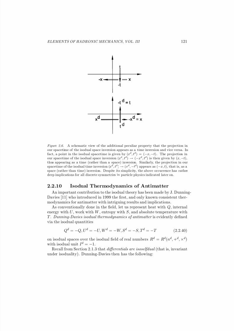
Figure 2.6. A schematic view of the additional peculiar property that the projection inour spacetime of the isodual space inversion appears as a time inversion and vice versa. Infact, a point in the isodual spacetime is given by (x

d, td) = (−x,−t). The projection in

our spacetime of the isodual space inversion ( xd

, td) → (−x

d, td) is then given by (x,−t),

thus appearing as a time (rather than a space) inversion. Similarly, the projection in ourspacetime of the isodual time inversion (x

d, td) → (x

d,−t

d) appears as (−x, t), that is, as aspace (rather than time) inversion. Despite its simplicity, the above occurrence has rather

deep implications for all discrete symmetries in particle physics indicated later on.

2.2.10 Isodual Thermodynamics of Antimatter

An important contribution to the isodual theory has been made by J. Dunning-Davies [11] who introduced in 1999 the first, and only known consistent ther-modynamics for antimatter with intriguing results and implications.

As conventionally done in the field, let us represent heat with Q, internalenergy with U , work with W , entropy with S , and absolute temperature withT . Dunning-Davies isodual thermodynamics of antimatter is evidently definedvia the isodual quantities

Qd

= −Q, U d

= −U, W d

= −W, S d

= −S, T d

= −T (2.2.40)

on isodual spaces over the isodual field of real numbers Rd = Rd(nd, +d, ×d)with isodual unit I d = −1.

Recall from Section 2.1.3 that differentials are isoselfdual (that is, invariantunder isoduality). Dunning-Davies then has the following:



122

THEOREM 2.2.1 [21]: Thermodynamical laws are isoselfdual.

Proof. For the First Law of thermodynamics we have

dQ = dU − dW ≡ ddQd = ddU d − ddW d. (2.2.41)

Similarly, for the Second Law of thermodynamics we have

dQ = T × dS ≡ ddQd = T d ×d S d, (2.2.42)

and the same occurs for the remaining laws. q.e.d.

Despite their simplicity, Dunning-Davies results [21] have rather deep im-plications. First, the identity of thermodynamical laws, by no means, impliesthe identity of the thermodynamics of matter and antimatter. In fact, in

Dunning-Davies isodual thermodynamics the entropy must always decrease in time, since the isodual entropy is always negative and is defined in a spacewith evolution backward in time with respect to us. However, these featuresare fully equivalent to the conventional increase of the entropy tacitly referredto positive units.

Also, Dunning-Davies results indicate that antimatter galaxies and quasarscannot be distinguished from matter galaxies and quasars via the use of ther-modynamics, evidently because their laws coincide, in a way much similar tothe identity of the trajectories of particles and antiparticles of Lemma 2.2.1.

This result indicates that the only possibility known at this writing to de-termine whether far-away galaxies and quasars are made up of matter or of antimatter is that via the predicted gravitational repulsion of the light emitted

by antimatter called isodual light (see next section and Chapter 5).

2.2.11 Isodual General Relativity

For completeness, we now introduce the isodual general relativity for theclassical gravitational representation of antimatter. A primary motivationfor its study is the incompatibility with antimatter of the positive-definitecharacter of the energy-momentum tensor of the conventional general relativitystudied in Chapter 1.

The resolution of this incompatibility evidently requires a structural revisionof general relativity [33] for a consistent treatment of antimatter. The only solution known to the author is that offered by isoduality.4

It should be stressed that this study is here presented merely for complete-ness, since the achievement of a consistent treatment of negative-energies, by

4The author would be grateful to colleagues who care to bring to his attention other “classical” grav-itational theories of antimatter compatible with the negative-energy solutions needed by antimatter.




no means, resolves the serious inconsistencies of gravitation on a Rieman-nian space caused by curvature, as studied in Section 1.2, thus requiring newgeometric vistas beyond those permitted by the Riemannian geometry (seeChapters 3 and 4).

As studied in Section 2.1.7, the isodual Riemannian geometry is definedon the isodual field Rd(nd, +d, ×d) for which the norm is negative–definite,Eq. (2.1.18). As a result, all quantities that are positive in Riemannian geom-etry become negative under isoduality, thus including the energy-momentum tensor .

In fact, the energy-momentum tensor of isodual electromagnetic waves(2.2.37) is negative-definite [8,9]

T dµν = (4 × π)−1d×d (F dµα×dF dαν + (1/4)−1d×d gdµν ×dF dαβ ×

dF dαβ ). (2.2.43)

The Einstein-Hilbert isodual equations for antimatter in the exterior condi-tions in vacuum are then given by [6, 9]

Gdµν = Rd

µν −1

2

d

×d gdµν ×d Rd = kd ×d T dµν , (2.2.44)

The rest of the theory is then given by the use of the isodual Riemanniangeometry of Section 2.1.7.

The explicit study of this gravitational theory of antimatter is left to theinterested reader due to the indicated inconsistencies of gravitational theorieson a Riemannian space for the conventional case of matter (Section 1.2). Theseinconsistencies multiply when treating antimatter, as we shall see.

2.3 OPERATOR ISODUAL THEORY OFPOINT-LIKE ANTIPARTICLES

2.3.1 Basic Assumptions

In this section we study the operator image of the classical isodual theory of the preceding section; we prove that the operator image of isoduality is equiv-alent to charge conjugation; and we show that isodual mathematics resolvesall known objections against negative energies.

A main result of this section is the identification of a simple, structurallynew formulation of quantum mechanics known as isodual quantum mechanicsor, more properly, as the isodual branch of hadronic mechanics first proposedby Santilli in Refs. [5]. Another result of this section is the fact that all numer-ical predictions of operator isoduality coincide with those obtained via chargeconjugation on a Hilbert space, thus providing the experimental verificationof the isodual theory of antimatter at the operator level.

Despite that, the isodual image of quantum mechanics is not trivial becauseof a number of far reaching predictions we shall study in this section and in



124

the next chapters, such as: the prediction that antimatter emits a new lightdistinct from that of matter; antiparticles in the gravitational field of matterexperience antigravity; bound states of particles and their antiparticles canmove backward in time without violating the principle of causality; and otherpredictions.

Other important results of this section are a new interpretation of the con-ventional Dirac equation that escaped detection for about one century, aswell as the indication that the isodual theory of antimatter originated fromthe Dirac equation itself, not so much from the negative-energy solutions, butmore properly from their two-dimensional unit that is indeed negative-definite,I 2×2 = Diag.(−1, −1).

As we shall see, Dirac’s “hole theory”, with the consequential restriction of the study of antimatter to the sole second quantization and resulting scientific

imbalance indicated in Section 1.1, were due to Dirac’s lack of knowledge of amathematics based on negative units.Intriguingly, had Dirac identified the quantity I 2×2 = Diag.(−1, −1) as the

unit of the mathematics treating the negative energy solutions of his equation,the physics of the 20-th century would have followed a different path because,despite its simplicity, the unit is indeed the most fundamental notion of allmathematical and physical theories.

2.3.2 Isodual Quantization

The isodual Hamiltonian mechanics (and its underlying isodual symplecticgeometry [5a] not treated in this chapter for brevity) permit the identificationof a new quantization channel, known as the naive isodual quantization [6] that

can be readily formulated via the use of the Hamilton-Jacobi-Santilli isodualequations (2.2.21) as follows

A◦d → −id ×d hd ×d Lndψd(td, rd), (2.3.1a)

∂ dA◦d/d∂ dtd + H d = 0 → id ×d ∂ dψd/d∂ dtd =

= H d ×d ψd = E d ×d ψd, (2.3.1b)

∂ dA◦d/d∂ dxdk − ˆ pk = 0 → pdk ×d ψd = −id ×d ∂ dkψd, (2.3.1c)

∂ dA◦d/d∂ d pdk = 0 → ∂ dψd/d∂ d pdk = 0. (2.3.1d)

Recall that the fundamental unit of quantum mechanics is Planck’s constanth = +1. It then follows that the fundamental unit of the isodual operator

theory is the new quantityhd = −1. (2.3.2)

It is evident that the above quantization channel identifies the new mechan-ics known as isodual quantum mechanics, or the isodual branch of hadronicmechanics.




2.3.3 Isodual Hilbert Spaces

Isodual quantum mechanics can be constructed via the anti-unitary trans-form

U × U † = hd = I d = −1, (2.3.3)

applied, for consistency, to the totality of the mathematical and physical for-mulations of quantum mechanics. We recover in this way the isodual real andcomplex numbers

n → nd = U × n × U † = n × (U × U †) = n × I d, (2.3.4)

isodual operatorsA → U × A × U † = Ad, (2.3.5)

the isodual product among generic quantities A, B (numbers, operators, etc.)

A × B → U × (A × B) × U † =

= (U × A × U †) × (U × U †)−1 × (U × B × U †) = Ad ×d Bd, (2.3.6)

and similar properties.Evidently, isodual quantum mechanics is formulated in the isodual Hilbert

space Hd with isodual states [6]

|ψ >d= −|ψ >†= − < ψ|, (2.3.7)

where < ψ| is a conventional dual state on H, and isodual inner product

< ψ|d × (−1) × |ψ >d ×I d, (2.3.8)

with isodual expectation values of an operator Ad

< Ad >d= (< ψ|d ×d Ad ×d |ψ >d /d < ψ|d ×d |ψ >d), (2.3.9)

and isodual normalization

< ψ|d ×d |ψ >d= −1. (2.3.10)

defined on the isodual complex field C d with unit −1 (Section 2.1.1).The isodual expectation values can also be reached via anti-unitary trans-

form (2.3.3),

< ψ| × A × |ψ >→ U × (< ψ| × A × |ψ >) × U †

=

= (< ψ| × U †) × (U × U †)−1 × (U × A × U †) × (U × U †)−1×

×(U × |ψ >) × (U × U †) =< ψ|d ×d Ad ×d |ψ >d ×I d. (2.3.11)

The proof of the following property is trivial.



126

LEMMA 2.3.1 [5b]: The isodual image of an operator A that is Hermitean on H over C is also Hermitean on Hd over C d (isodual Hermiticity).

It then follows that all quantities that are observables for particles areequally observables for antiparticles represented via isoduality.

LEMMA 2.3.2 [5b]: Let H be a Hermitean operator on a Hilbert space Hover C with positive-definite eigenvalues E ,

H × |ψ >= E × |ψ >, H = H †, E => 0. (2.3.12)

Then, the eigenvalues of the isodual operator H d on the isodual Hilbert spaceHd over C d are negative-definite,

H d ×d |ψ >d= E d ×d |ψ >d, H d = H d†d, E d < 0. (2.3.13)

This important property establishes an evident compatibility between theclassical and operator formulations of isoduality.

We also mention the isodual unitary laws

U d ×d U d†

= U d†

×d U d = I d, (2.3.14)

the isodual traceT rdAd = (T rAd) × I d ∈ C d, (2.3.15a)

T rd(Ad ×d Bd) = T rdAd ×d T rdBd, (2.3.15b)

the isodual determinant DetdAd = (DetAd) × I d ∈ C d, (2.3.16a)

Detd(Ad ×d Bd) = Detd ×d DetdBd, (2.3.16b)

the isodual logarithm of a real number n

Logdnd = −(Log nd) × I d, (2.3.17)

and other isodual operations.The interested reader can then work out the remaining properties of the

isodual theory of linear operators on a Hilbert space.

2.3.4 Isoselfduality of Minkowski’s Line Elements andHilbert’s Inner Products

A most fundamental new property of the isodual theory, with implicationsas vast as the formulation of a basically new cosmology, is expressed by thefollowing lemma whose proof is a trivial application of transform (2.3.3).




LEMMA 2.3.3 [23]: Minkowski’s line elements and Hilbert’s inner productsare invariant under isoduality (or they are isoselfdual according to Definition 2.1.2),

x2 = (xµ × ηµν × xν ) × I ≡

≡ (xdµ ×d ηdµν ×d xdν ) × I d = xd

2d, (2.3.18a)

< ψ| × |ψ > × I ≡ < ψ|d ×d |ψ >d × I d. (2.3.18b)

As a result, all relativistic and quantum mechanical laws holding for matter also hold for antimatter under isoduality. The equivalence of charge conjuga-tion and isoduality then follows, as we shall see shortly.

Lemma 2.3.3 illustrates the reason why isodual special relativity and isodualHilbert spaces have escaped detection for about one century. Note, however,

that invariances (2.3.18) require the prior discovery of new numbers, thosewith negative unit.

2.3.5 Isodual Schrodinger and Heisenberg’s Equations

The fundamental dynamical equations of isodual quantum mechanics arethe isodual images of conventional dynamical equations. They are todayknown as the Schr¨ odinger-Santilli isodual equations [4] (where we assumehereon hd = −1, thus having ×dhd = 1)

id ×d ∂ |ψ >d /d∂ dtd = H d ×d |ψ >d, (2.3.19a)

pdk ×d |ψ >d= −id ×d ∂ d|ψ >d /d∂ drd, (2.3.19b)

and the Heisenberg-Santilli isodual equations

id ×d ddAd/dddtd = Ad ×d H d − H d ×d Ad = [Ad, H d]d, (2.3.20a)

[rdi , pd j ]d = id ×d δdi j , [rd, rdj]d = [ pdi , pd j ]d = 0. (2.3.20b)

Note that, when written explicitly, Eq. (2.3.19a) is based on an associativemodular action to the left,

− < ψ | ×d H d = (∂ d < ψ|∂ dtd) ×d id, (2.3.21)

It is an instructive exercise for readers interested in learning the new me-chanics to prove the equivalence of the isodual Schrodinger and Heisenberg

equations via the anti-unitary transform (2.3.3).



128

2.3.6 Isoselfdual Re-Interpretation of Dirac’s

EquationIsoduality has permitted a novel interpretation of the conventional Diracequation (we shall here used the notation of Ref. [12]) in which the negative-energy states are reinterpreted as belonging to the isodual images of positiveenergy states, resulting in the first known consistent representation of antipar-ticles in first quantization.

This result should be expected since the isodual theory of antimatter appliesat the Newtonian level, let alone that of first quantization. Needless to say,the treatment via isodual first quantization does not exclude that via isodualsecond quantization. The point is that the treatment of antiparticles is nolonger restricted to second quantization, as a condition to resolve the scientificimbalance between matter and antimatter indicated earlier.

Consider the conventional Dirac equation [2]

[γ µ × ( pµ − e × Aµ/c) + i × m] × Ψ(x) = 0, (2.3.22)

with realization of Dirac’s celebrated gamma matrices

γ k =

0 −σk

σk 0

, γ 4 = i ×

I 2×2 0,

0 −I 2×2

, (2.3.23a)

{γ µ, γ ν } = 2×ηµν , Ψ = i ×

Φ

−Φ†

, (2.3.23b)

At the level of first quantization here considered, the above equation is

rather universally interpreted as representing an electron under an externalelectromagnetic field.The above equations are generally defined in the 6-dimensional space given

by the Kronecker product of the conventional Minkowski spacetime and aninternal spin space

M Tot = M (x,η,R) × S spin, (2.3.24)

with total unitI Tot = I orb × I spin =

= Diag.(1, 1, 1, 1) × Diag.(1, 1), (2.3.25)

and total symmetryP (3.1) = SL(2.C ) × T (3.1). (2.3.26)

The proof of the following property is recommended to interested readers.THEOREM 2.3.1 [5b]: Pauli’s sigma matrices and Dirac’s gamma matrices

are isoselfdual ,σk ≡ σdk, (2.3.27a)




γ µ ≡ γ dµ. (2.3.27b).

The above properties imply an important re-interpretation of Eqs. (2.3.22),first identified in Ref. [9] and today known as the Dirac-Santilli isoselfdual equation, that can be written

[γ µ × ( pµ − e × Aµ/c) + i × m] × Ψ(x) = 0, (2.3.28)

with re-interpretation of the gamma matrices

γ k =

0 σdk

σk 0

, γ 4 = i

I 2×2 0,

0 I d2×2

, (2.3.29a)

{γ µ, γ ν } = 2d×dηdµν , Ψ = −γ 4 × Ψ = i ×

Φ

Φd

, (2.3.29b)

By recalling that isodual spaces coexist with, but are different from conven-tional spaces, we have the following:

THEOREM 3.3.2 [9]: The Dirac-Santilli isoselfdual equation is defined on the 12-dimensional isoselfdual representation space

M Tot = {M (x,η,R) × S spin} × {M d(xd, ηd, Rd) ×d S dspin}, (2.3.30)

with isoselfdual total 12-dimensional unit

I Tot = {I orb × I spin} × {I dorb ×d I dspin}, (2.3.31)

and its symmetry is given by the isoselfdual product of the Poincare symmetry and its isodual

S Tot = P (3.1) × P d(3.1) =

= {SL(2.C ) × T (3.1)} × {SLd(2.C d) ×d T d(3.1)}. (2.3.32)

A direct consequence of the isoselfdual structure can be expressed as follows.

COROLLARY 2.3.2a [9]: The Dirac-Santilli isoselfdual equation providesa joint representation of an electron and its antiparticle (the positron) in first quantization,

Dirac Equation = Electron × Positron (2.3.33)

In fact, the two-dimensional component of the wave function with positive-energy solution represents the electron and that with negative-energy solutionsrepresent the positron without any need for second quantization, due to thephysical behavior of negative energies in isodual treatment established earlier.

Note the complete democracy and equivalence in treatment of the electronand the positron in equation (2.3.28), in the sense that the equation can be



130

equally used to represent an electron or its antiparticle. By comparison, ac-cording to the original Dirac interpretation, the equation could only be usedto represent the electron [12], since the representation of the positron requiredthe “hole theory”.

It has been popularly believed throughout the 20-th century that Dirac’sgamma matrices provide a “four-dimensional representation of the SU(2)-spinsymmetry”. This belief is disproved by the isodual theory, as expressed by thefollowing

THEOREM 3.3.3 [5b]: Dirac’s gamma matrices characterize the direct prod-uct of an irreducible two-dimensional (regular) representation of the SU(2)-spin symmetry and its isodual,

Diracs Spin Symmetry : SU (2)×

SU d(2). (2.3.34)

In fact, the gamma matrices are characterized by the conventional, 2-dim-ensional Pauli matrices σk and related identity I 2×2 as well as other matricesthat have resulted in being the exact isodual images σdk with isodual unit I d2×2.

It should be recalled that the isodual theory was born precisely out of theseissues and, more particularly, from the incompatibility between the popularinterpretation of gamma matrices as providing a “four-dimensional” repre-sentation of the SU(2)-spin symmetry and the lack of existence of such a representation in Lie’s theory.

The sole possibility known to the author for the reconciliation of Lie’s theoryfor the SU(2)-spin symmetry and Dirac’s gamma matrices was to assume that−I

2×2is the unit of a dual-type representation. The entire theory studied in

this chapter then followed.It should also be noted that, as conventionally written, Dirac’s equation

is not isoselfdual because not sufficiently symmetric in the two-dimensionalstates and their isoduals.

In summary, Dirac’s was forced to formulate the “hole theory” for antiparti-cles because he referred the negative energy states to the conventional positiveunit, while their reformulation with respect to negative units yields fully phys-ical results.

It is easy to see that the same isodual reinterpretation applies for Majorana’sspinorial representations [13] (see also [14,15]) as well as Ahluwalia’s broaderspinorial representations (1/2, 0)+(0, 1/2) [16] (see also the subsequent paper

[17]), that are reinterpreted in the isoselfdual form (1, 2, 0) + (1, 2, 0)d

, thusextending their physical applicability to first quantization.In the latter reinterpretation the representation (1/2,0) is evidently done

conventional spaces over conventional fields with unit +1, while the isodualrepresentation (1/2, 0)d is done on the corresponding isodual spaces defined




on isodual fields with unit −1. As a result, all quantities of the representation(1/2,0) change sign under isoduality.

It should be finally indicated that Ahluwalia treatment of Majorana spinorshas a deep connection with isoduality because the underlying Class II spinorshave a negative norm [16] precisely as it is the case for isoduality. As a re-sult, the isodual reinterpretation under consideration here is quite natural andactually warranted for mathematical consistency, e.g., to have the topologycharacterized by a negative norm be compatible with the underlying fields.

2.3.7 Equivalence of Isoduality and chargeconjugation

We come now to another fundamental point of this chapter, the proof thatisoduality is equivalent to charge conjugation. This property is crucial for the

experimental verification of isoduality at the particle level too. This equiv-alence was first identified by Santilli in Ref. [6] and can be easily expressedtoday via the following:

LEMMA 2.3.4 [6,5b,18]: The isodual transform is equivalent to charge conjugation.

Proof. Charge conjugation is characterized by the following transform of wavefunctions (see, e.g., Ref. [12], pages 109 and 176)

Ψ(x) → C Ψ(x) = c × Ψ†(x), (2.3.35)

where|c| = 1, (2.3.36)

thus being manifestly equivalent to the isodual transform

Ψ(x) → Ψd(xd) = −Ψ†(−xt), (2.3.37)

where t denotes transpose.A reason why the two transforms are equivalent, rather than identical, is

the fact that charge conjugation maps spacetime into itself, while isodualitymaps spacetime into its isodual. q.e.d.

Let us illustrate Lemma 2.3.4 with a few examples. As well known, theKlein-Gordon equation for a free particle

∂ µ∂ µΨ − m2 × Ψ = 0, (2.3.38)

is invariant under charge conjugation, in the sense that it is turned into theform

c × [Ψ∂ µ∂ µ − Ψ × m2] = 0, |c| = 1, (2.3.39)



132

where the upper bar denotes complex conjugation (since Ψ is a scalar), while

the Lagrangian densityL = −(h × h/2 × m) × {∂ µΨ − i × e × Aµ/h × c) × Ψ]×

×[∂ Ψ + (i × e × Aµ/h × c) × Ψ] + m × m × Ψ × Ψ, (2.3.40)

is left invariant and the four-current

J µ = −(i × h/2 × m) × [ψ × ∂ µΨ − (∂ µΨ) × Ψ], (2.3.41)

changes signJ µ → CJ µ = −J µ. (2.3.42)

By recalling the selfduality of ordinary derivatives, Eq. (2.1.30), under

isoduality the Klein-Gordon Equation becomes

[∂ µ∂ µΨ − m2 × Ψ]d = Ψd∂ dµ∂ dµ − Ψd ×d md ×d md =

= −[Ψ∂ µ∂ µ − Ψ × m2] = 0, (2.3.43)

thus being equivalent to Eq. (2.3.39), while the Lagrangian changes sign andthe four-current changes sign too,

J dµ = −(i × h/2 × m) × [Ψ × ∂ µΨ − (∂ µΨ) × Ψ]d =

= (i × h/2 × m) × [Ψ × ∂ µΨ − (∂ µΨ) × Ψ], (2.3.44)

(where we have used the isoselfduality of the imaginary number i).

The above results confirm Lemma 2.3.4 because of the equivalent behaviorof the equations of motion and the four-current, while the change of sign of the Lagrangian does not affect the numerical results.

As it is also well known, the Klein-Gordon equation for a particle under anexternal electromagnetic field [12]

[(∂ µ + i × e × Aµ/h × c)×

×(∂ µ + i × e × Aµ/h × c) − m2] × Ψ = 0, (2.3.45)

is equally invariant under charge conjugation in which either e or Aµ changesign, in view of the known invariance

C (i × e × Aµ/h × c) = i × e × Aµ/h × c, (2.3.46)

while the four-current also changes sign. By noting that the preceding invari-ance persists under isoduality,

(i × e × Aµ/h × c)d = i × e × Aµ/h × c, (2.3.47)




Eq. (2.3.45) remains invariant under isoduality, while the Lagrangian densitychanges sign and the four-current, again, changes sign.

Similarly, consider Dirac equation (see also Ref. [12], pp. 176-177)

[γ µ × (∂ µΨ − (i × e × Aµ/h × c) × Ψ + m × Ψ = 0, (2.3.48)

with Lagrangian density

L = (h × c/2) × {Ψ × γ µ × [∂ µΨ + (i × e × Aµ/h × c) × Ψ]−

−(∂ µΨ − (i × e × Aµ/h × c) × Ψ] × γ µ − m × Ψ × Ψ (2.3.49a)

Ψ = Ψ† × γ 4, (2.3.49b)

and four-current

J µ = i × c × Ψ × γ µ × Ψ = i × c × Ψ† × γ 4 × γ µ × Ψ (2.3.50)

The charge conjugation for Dirac’s equations is given by the transform [12]

Ψ → C Ψ = c × S −1C × Ψt (2.3.51)

where S C is a unitary matrix such that

γ µ → −γ tµ = S C × γ µ × S −1c , (2.3.52)

and there is the change of sign either of e or of Aµ, under which the equationis transformed into the form

[∂ µΨ − (i × e × Aµ/h × c) × Ψ] × γ µ

− m × Ψ = 0, (2.3.53)

while the Lagrangian density changes sign and the four-current remains thesame,

L → CL = −L, J µ → CJ µ = J µ. (2.3.54)

It is easy to see that isoduality provides equivalent results. In fact, for Eq.(2.3.48) we have

{[γ µ × (∂ µΨ − i × e × Aµ/h × c) × Ψ + m × Ψ}d =

= [∂ µΨ† − (i × e × Aµ/h × c) × Ψ†] × γ µ − m × Ψ† = 0, (2.3.55)

that, when multiplied by γ 4 reproduces Eq. (2.3.53) identically. Similarly, by

recalling that Dirac’ s gamma matrices are isoselfdual (Theorem 2.3.1), andby noting that

Ψd = (Ψ† × γ 4)d = γ 4 × Ψ, (2.3.56)

we haveLd = L (2.3.57)



134

while for the four-current we have

J dµ = −i × c × Ψ† × γ µ × γ 4 × ψ. (2.3.58)

But the γ µ and γ 4 anticommute. As a consequence, the four-current does notchange sign under isoduality as in the conventional case.

Note that the lack of change of sign under isoduality of Dirac’s four-currentJ µ confirms reinterpretation (2.3.28) since, for the latter equation, the totalcharge is null.

The equivalence between isoduality and charge conjugation of other equa-tions, such as those by Weyl, Majorana, etc., follows the same lines.

2.3.8 Experimental Verification of the Isodual Theoryof Antimatter in Particle Physics

In Section 2.2.3. we have established the experimental verification of theisodual theory of antimatter in classical physics. That in particle physicsrequires no detailed elaboration since it is established by the equivalence of charge conjugation and isoduality (Lemma 2.3.4), and we can write:

LEMMA 2.3.5 [6,5b,18], [7]: All experimental data currently available for antiparticles represented via charge conjugation are equally verified by the iso-dual theory of antimatter.

2.3.9 Elementary Particles and their Isoduals

We assume the reader is familiar with the conventional definition of elemen-

tary particles as irreducible unitary representations of the spinorial coveringof the Galilei symmetry G(3.1) for nonrelativistic treatments and those of thePoincare symmetry P (3.1) for relativistic treatments. We therefore introducethe following:

DEFINITION 2.3.1: Elementary isodual particles (antiparticles) are given by irreducible unitary representations of the spinorial covering of the Galilei-Santilli’s isodual symmetry Gd(3.1) for nonrelativistic treatments and those of the Poincare-Santilli isodual symmetry P d(3.1) for relativistic treatments.

A few comments are now in order. First, one should be aware that “isod-ual particles” and “antiparticles” do not represent the same notion, evidentlybecause of the negative mass, energy and time of the former compared topositive mass, energy and time of the latter. In the rest of this chapter, un-less otherwise stated, the word “antiparticle” will be referred to the “isodualparticle.”




For instance the word “positron” e+ is more appropriately intended to rep-

resent the “isodual electron” with symbol e

−d

. Similarly the, “antiproton” p

−

is intended to represent the “isodual proton” p+d.Second, the reader should note the insistence on the elementary character

of the antiparticles here admitted. The reason is that the antigravity studiedin Chapter 4 is specifically formulated for “elementary” isodual particles, suchas the isodual electron, due to a number of unsettled aspects pertaining tocomposite particles.

Consider, as an illustration, the case of mesons. If the π◦ is a bound state of a particle and its isodual, the state is isoselfdual and, as such, it cannot expe-rience antigravity, as illustrated in the next section. A number of ambiguitiesthen follow for the study of the gravity of the charged mesons π±, such as theproblem of ascertaining which of the two mesons is a particle and which is its

isodual or, whether the selected antiparticle is indeed the isodual image of theparticle as a necessary condition for meaningful study of their gravity.Note that essentially the same ambiguities prohibit the use of muons for

a serious theoretical and experimental studies of the gravity of antiparticles,again, because of unsettled problems pertaining to the structure of the muonsthemselves. Since the muons are naturally unstable, they cannot be crediblybelieved to be elementary. Therefore, serious theoretical and experimentalstudies on the gravity of muons require the prior identification of their con-stituents with physical particles.

Finally, the reader should be aware that Definition 2.3.1 excludes the use of quark conjectures for the gravitational studies of this monograph. This is dueto the well-known basic inconsistency of quark conjecture of not admitting

any gravitation at all (see, e.g., the Appendix of Ref. [18]). In fact, gravitycan only be defined in our spacetime while quarks can only be defined intheir mathematical unitary internal space with no known connection with ourspacetime due to the O’Rafearthaigh theorem.5

Also, the only “masses” that can be credibly claimed as possessing iner-tia are the eigenvalues of the second-order Casimir invariant of the Poincaresymmetry pµ × pµ = m2. Quarks cannot be characterized via such a fun-damental symmetry, as well known. It then follows that “quark masses” aremere mathematical parameters defined in the mathematical internal complex-unitary space that cannot possibly be used as serious basis for gravitationaltests.

5The p ossible connection between internal and spacetime symmetries offered by supersymmetrictheories cannot be credibly used for gravitational tests due to their highly unsettled character andthe prediction of a zoo of new particles none of which has been experimentally detected to theauthor’s best knowledge.



136

2.3.10 Photons and their Isoduals

As it is well known, photons have no charge and, therefore, they are in-variant under charge conjugation, as transparent from the simple plane-waverepresentation

Ψ(t, r) = N × ei×(k×r−E ×t), N ∈ R, (2.3.59)

with familiar relativistic form

Ψ(x) = N × ei×kµ×xµ

, (2.3.60)

and familiar expression for the energy

E = h × ν. (2.3.61)

As a result, matter and antimatter have been believed throughout the 20-

th century to emit the same light. In turn, this belief has left fundamentallyunsettled basic questions in astrophysics and cosmology, such as the lack of quantitative studies as to whether far-away galaxies and quasars are made upof matter or of antimatter.

One of the most intriguing and far reaching implications of the isodual the-ory is that, while remaining evidently invariant under charge conjugation, thephoton is not invariant under isoduality, thus admitting a conjugate particlefirst submitted by Santilli in Ref. [18] under the name of isodual photon. Inparticular, the isodual photon emerges as having physical characteristics thatcan be experimentally measured as being different from those of the photon.

Therefore, the isodual theory offers the first known possibilities of quanti-tative theoretical and experimental studies as to whether a far-away galaxy or

quasar is made of matter or of antimatter due to detectable physical differencesof their emitted light.

Note that the term “antiphoton” could be misleading because the prefix“anti” is generally assumed as referring to charge conjugation. For this rea-son the name of “isodual photon” appears to be preferable, also because itrepresents, more technically, the intended state.

In fact, the photon is mapped by isoduality into a new particle possessingall negative-definite physical characteristics, with the following simple isodualplane-wave representation

Ψd(td, rd) = N d ×d eid×d(kd×drd−E d×dtd)d , N d ∈ Rd, (2.3.62)

with relativistic expression on isodual Minkowski space

Ψd(xd) = N d ×d eid×dkdµ×

dxdµ

d , (2.3.63)

and isodual expression for the energy

E d = hd ×d ν d, (2.3.64)




where ed is the isodual exponentiation (2.1.26b).Note that, since i is isoselfdual, Eq. (2.1.20), the exponent of the plane-

wave representation is invariant under both charge conjugation and isoduality,as illustrated by the following expression

id ×d (kd ×d rd − E d ×d td) ≡ i × (k × r − E × t), (2.3.65)

or its relativistic counterpart

id ×d kdµ ×d xdµ ≡ i × kµ × xµ. (2.3.66)

thus confirming the lack of contradiction between charge conjugation and iso-duality.

Moreover, both the photon and the isodual photon travel in vacuum withthe same (absolute) speed |c|, for which we have the additional identity

kdµ ×d kdµ ≡ kµ × kµ = 0. (2.3.67)

Despite the above identities, energy and time are positive-definite for thephoton, while they are negative-definite for the isodual photon. As we shallsee, the latter property implies that photons are attracted by the gravitationalfield of matter while isodual photons are repelled, thus providing a physicallydetectable difference.

Additional differences between light emitted by matter and that emitted byantimatter, such as those pertaining to parity and other discrete symmetries,require additional study.

2.3.11 Electrons and their IsodualsThe next truly elementary particles and antiparticles are the electron e− and

its antiparticle, the positron e+ or the isodual electron e−d. The differencesbetween the “positron” and the “isodual electron” should be kept in mind. Infact, the former has positive rest energy and moved forward in time, while thelatter has negative rest energy and moves backward in time.

Also, the electron is known to experience gravitational attraction in thefield of matter, as experimentally established. As conventionally defined, thepositron too is predicted to experience gravitational attraction in the field of matter (because its energy is positive).

However, as we shall see in Chapter 4, the isodual electron is predicted toexperience antigravity when immersed in the field of matter, and this illus-trates again the rather profound physical differences between the “positron”and the “isodual electron”.

Note that, in view of their truly elementary character, isodual electrons arethe ideal candidates for the measurement of the gravitational field of antipar-ticles.



138

2.3.12 Protons and their Isoduals

The next particles demanding comments are the proton p+

, the antiproton p− and the isodual proton p+d. In this case the differences between the “an-tiproton” and the “isodual proton” should be kept in mind to avoid majorinconsistencies with the isodual theory, such as the study of the possible anti-gravity for antiprotons in the field of matter which antigravity cannot existfor the isodual theory (due, again, to the positive mass of the antiproton).

Note that these particles are not elementary and, as such, they are not ad-mitted by Definition 2.3.1. moreover, as stressed earlier [18], when representedin term of quark conjectures both the proton and the antiproton cannot admitany gravity at all, let alone antigravity. As a result, extreme scientific careshould be exercised before extending to all antimatter any possible gravita-tional measurements for antiprotons.

2.3.13 The Hydrogen Atom and its Isodual

The understanding of this chapter requires the knowledge that studies con-ducted on the antihydrogen atom (see, e.g., the various contributions in Pro-ceedings [19]), even though evidently interesting per se, they have no con-nection with the isodual hydrogen atom, because the antihydrogen atom haspositive mass, for which antigravity is prohibited, and emits conventional pho-tons. Therefore, it is important to inspect the differences between these twoformulations of the simplest possible atom of antimatter.

We assume as exactly valid the conventional quantum mechanical theory of bound states of point-like particles at large mutual distances,6 as available inquantum mechanical books so numerous to discourage even a partial listing.

For the case of two particles denoted with the indices 1, 2, the total statein the Hilbert space is the familiar tensorial product of the two states

|ψ >= |ψ1 > ×|ψ2 > . (2.3.68)

The total Hamiltonian H is the sum of the kinetic terms of each state plusthe familiar interaction term V (r) depending on the mutual distance r,

H = p1 × p1/2 × m1 + p2 × p2/2 × m2 + V (r). (2.3.69)

The total angular momentum is computed via the familiar expressions forangular momenta and spins

J = J 1 × I + I × J 2, S = S 1 × I + I × S 2, (2.3.70)

6We are here referring to the large mutual distances as occurring in the atomic structure and excludethe short mutual distances as occurring in the structure of hadrons, nuclei and stars since a seriousstudy of the latter is dramatically beyond the capabilities of quantum mechanics, as shown beyondscientific doubt in Chapter 3.




where the I s are trivial units, with the usual rules for couplings, addition,etc. One should note that the unit for angular momenta is three-dimensionalwhile that for spin has a generally different dimension.

A typical example of two-body bound states of particles is the hydrogen atom that experiences attraction in the gravitational field of matter with thewell established emission of conventional photons.

The study of bound states of point-like isodual particles at large mutual distances is an important part of isodual quantum mechanics. These boundstates can be studied via an elementary isoduality of the corresponding boundstates for particles, that is, via the use of the isodual Hilbert spaces Hd studiedearlier.

The total isodual state is the tensorial product of the two isodual states

|ψd(rd) >d= |ψd

1(rd) >d ×d|ψd

2(rd) >d= − < ψ

1(−r)|× < ψ

2(−r)|. (2.3.71)

The total isodual Hamiltonian is the sum of the isodual kinetic terms of eachparticle plus the isodual interaction term depending on the isodual mutualdistance,

H d = pd1 ×d pd1/d2d ×d md1 + pd2 ×d pd2/d2d ×d md

2 + V d(rd). (2.3.72)

The total isodual angular momentum is based on the expressions for isodualangular momenta and spin

J d = J d1 ×d I d + I d ×d J d2 , (2.3.73a)

S d = S d

1

×d I d + I d ×d S d

2, (2.3.73b)

The remaining aspects (couplings, addition theory of angular momenta,etc.) are then given by a simple isoduality of the conventional theory that ishere omitted for brevity.

Note that all eigenvalues that are positive for the conventional case mea-sured with positive units become negative under isoduality, yet measured withnegative units, thus achieving full equivalence between particle and antiparti-cle bound states.

The simplest possible application of the above isodual theory is that for theisodual hydrogen atom (first worked out in Ref. [18]). The novel predictionsof isoduality over that of the antihydrogen atom is that the isodual hydrogenatom is predicted to experience antigravity in the field of matter and emits

isodual photons that are also repelled by the gravitational field of matter.

2.3.14 Isoselfdual Bound States

Some of the most interesting and novel bound states predicted by the isodualtheory are the isoselfdual bound states, that is, bound states that coincide with



140

their isodual image. The simplest case is the bound state of one elementaryparticle and its isodual, such as the positronium.

The condition of isoselfduality requires that the basic symmetry must beitself isoselfdual, e.g., for the nonrelativistic case the total symmetry must be

GTot = G(3.1) × Gd(3.1), (2.3.74)

where × is the Kronecker product (a composition of states thus being isoself-dual), with a simple relativistic extension here assumed as known from thepreceding sections.

The total unit must also be isoselfdual,

I Tot = I × I d, (2.3.75)

where I represents the space, time and spin units.The total Hilbert space and related states must also be isoselfdual,

HTot = H × Hd, (2.3.76a)

|ψ >Tot= |ψ > +|ψ >d= |ψ > − < ψ|, (2.3.76b)

and so on.A main feature is that isoselfdual states exist in both the spacetime of

particles and that of antiparticles. Therefore, the computation of the totalenergy must be done either in H, in which case the total energy is positive, or in Hd, in which case the total energy is negative.

Suppose that a system of one elementary particle and its isodual is studied

in our laboratory of matter. In this case the eigenvalues for both particle andits isodual must be computed in H, in which case we have the equation

i × ∂ t|ψ >= ( p × p/2 × m) × |ψ > +

+( pd ×d pd/d2s ×d md) ×d |ψ > +V (r) × |ψ > =

= [ p × p/2 × m + V (r)] × |ψ >= E × |ψ >, (2.3.77)

under which the total energy E is evidently positive.When the same isoselfdual state is detected in the spacetime of antimatter,

it must be computed with respect to Hd, in which case the total energy isnegative, as the reader is encouraged to verify.

The total angular momentum and other physical characteristics are com-puted along similar lines and they also result in having positive values whencomputed in H, as occurring for the conventional charge conjugation.

As we shall see shortly, the positive character of the total energy of boundstates of particles and their antiparticles is crucial for the removal of the in-consistencies of theories with negative energy.




The above properties of the isoselfdual bound states have the followingimplications:

1) Isoselfdual bound states of elementary particles and their isoduals arepredicted to be attracted in both, the gravitational field of matter and that of antimatter because their total energy is positive in our world and negative inthe isodual world. This renders necessary an experimental verification of thegravitational behavior of isoselfdual bound states, independently from thatof individual antiparticles. Note that the prediction holds only for boundstates of truly elementary particles and their isoduals, such as the positronium.No theoretical prediction for the muonium and the pionium is today feasiblebecause the unsettled nature of their constituents.

2) Isoselfdual bound states are predicted to have a null internal total timet + td = 0 and therefore acquires the time of the matter or antimatter in which

they are immersed, although the physical time t of the observer (i.e., of thebound state equation) is not null. This is readily understood by noting that thequantity t of Eq. (2.3.77) is our own time, i.e., we merely study the behaviorof the state with respect to our own time. A clear understanding illustratedpreviously with the “isodual cube” of Section 2.1 is that the description of astate with our own time, by no means, implies that its intrinsic time necessarilycoincides with our own. Note that a similar situation occurs for the energybecause the intrinsic total energy of the positronium is identically null, E +E d = 0. Yet the energy measured by us is E part. − E dantipart. = 2E > 0. Asimilar situation occurs for all other physical quantities.

3) Isoselfdual bound states may result in being the microscopic image of themain characteristics of the entire universe. Isoselfduality has in fact stimulated

a new cosmology, the isoselfdual cosmology [21] studied in Chapter 5, thatis patterned precisely along the structure of the positronium or of Dirac’sequation in our isoselfdual re-interpretation. In this case the universe resultsin having null total physical characteristics, such as null total energy, null totaltime, etc., thus implying no discontinuity at its creation.

2.3.15 Resolution of the Inconsistencies of NegativeEnergies

The treatment of antiparticles with negative energies was rejected by Diracbecause incompatible with their physical behavior. Despite several attemptsmade during the 20-th century, the inconsistencies either directly or indirectlyconnected to negative energies have remained unresolved.

The isodual theory of antimatter resolves these inconsistencies for the reasonnow familiar, namely, that the inconsistencies emerge when one refers negativeenergies to conventional numbers with positive units, while the same incon-sistencies cannot be evenly formulated when negative energies are referred toisodual numbers and their negative units.



142

A good illustration is given by the known objection according to whichthe creation of a photon from the annihilation of an electron-positron pair,with the electron having a positive energy and the positron having a negativeenergy, would violate the principle of conservation of the energy.

In fact, such a pair could be moved upward in our gravitational field withoutwork and then annihilated in their new upward position. The resulting photonwould then have a blueshift in our gravitational field of Earth, thus havingmore energy than that of the original photon.

Presumed inconsistencies of the above type cannot be even formulatedwithin the context of the isodual theory of antimatter because, as shown inthe preceding section, the electron-positron state is isoselfdual, thus having anon-null positive energy when observed in our spacetime. Consequently, thelifting upward of the pair does indeed require work and no violation of the

principle of conservation of the energy can be expected.A considerable search has established that all other presumed inconsisten-cies of negative energy known to the author cannot even be formulated withinthe context of the isodual theory of antimatter. Nevertheless, the author wouldbe particularly grateful to any colleague who bring to its attention inconsis-tencies of negative energies that are really applicable under negative units.




References

[1] R. M. Santilli, Hadronic J. 8, 25 and 36 (1985).

[2] R. M. Santilli, Algebras, Groups and Geometries 10, 273 (1993).

[3] J. V. Kadeisvili, Algebras, Groups and Geometries 9, 283 and 319 (1992).

[4] R. M. Santilli, Rendiconti Circolo Matematico di Palermo, Supplemento 42, 7 (1996).

[5] R. M. Santilli, Elements of Hadronic Mechanics, Vols. I: Mathematical Foundations,

[5a], II: Theoretical Foundations [5b], Ukrainian Academy of Sciences, Kiev, SecondEdition (1995).

[6] R. M. Santilli, Comm. Theor. Phys. 3, 153 (1993).

[7] R. M. Santilli, J. Moscow Phys. Soc. 3, 255 (1993).

[8] R. M. Santilli, Intern. J. Modern Phys. D 7, 351 (1998).

[9] R. M. Santilli, Intern. J. Modern Phys. A 14, 2205 (1999).

[10] D. V. Ahluwalia, M. B. Johson and T. Goldman, Phys. Letters B 316, 102 (1993).

[11] J. Dunning-Davies, Foundations of Physics Letters, 12, 593 (1999).

[12] E. Corinaldesi and F. Strocchi, Relativistic Wave Mechanics, North Holland, Amster-dam (1963).

[13] E. Majorana, Nuovo Cimento 14, 171 (1937).

[14] J. A. McLennan, jr., Phys. Rev. 106, 821 (1957).

[15] K. M. Case, Phys. Rev. 107, 307 (1957).

[16] D. V. Ahluwalia, Intern. J. Modern Phys. A 11, 1855 (1996).

[17] V. V. Dvoeglazov, Hadronic J. 20, 435 (1997).

[18] R. M. Santilli, Hyperfine Interactions, 109, 63 (1997).

[19] M. Holzscheiter, Editor, Proceedings of the International Workshop on Antimatter

Gravity , Sepino, Molise, Italy, May 1996, Hyperfine Interactions, Vol. 109 (1997) [2c].

[20] R. M. Santilli, contributed paper to New Frontiers in Hadronic Mechanics, T. L. Gill,Editor, Hadronic Press (1996), pages 343-416.

[21] R. M. Santilli, contributed paper to Proceedings of the International Workshop on

Modern Modified Theories of Gravitation and Cosmology, E. I. Guendelman, Editor,Hadronic Press, pages 113-169 (1998).

[22] R. M. Santilli, Journal of Dynamical Systems and Geometric Theories, 1, 121 (2003).

[23] J. V. Kadeisvili, Algebras, Groups and Geometries 9, 283 and 319 (1992).



144 ELEMENTS OF HADRONIC MECHANICS, VOL. III

[24] J. V. Kadeisvili, Math. Methods in Appl. Sci. 19, 1349 (1996).

[25] J. V. Kadeisvili, Acta Appl. Math. 50, 131 (1998).

[26] A. K. Aringazin, A. Jannussis, D. F. Lopez, M. Nishioka and B. Veljanosky, Santilli’s

Lie–Isotopic Generalization of Galilei’s Relativities, Kostarakis Publisher, Athens,Greece (1980) [10a].

[27] J. V. Kadeisvili, Santilli’s Isotopies of Contemporary Algebras, Geometries and Rela-

tivities, Second Edition, Ukrainian Academy of Sciences, Kiev (1997).

[28] D. S. Sourlas and G. T. Tsagas, Mathematical Foundations of the Lie-Santilli Theory ,Ukrainian Academy of Sciences, Kiev (1993).

[29] J. Lohmus, E. Paal and L. Sorgsepp, Nonassociative Algebras in Physics, HadronicPress, Palm Harbor, FL, (1994).

[30] R. M. Falcon Ganfornina and J. Nunez Valdes, Fondamentos de la Isoteoria de Lie-Santilli, (in Spanish) International Academic Press, America-Europe-Asia, (2001), alsoavailable in the pdf file http://www.i-b-r.org/docs/spanish.pdf.

[31] Chun-Xuan Jiang, Foundations of Santilli’s Isonumber Theory, with Applications to

New Cryptograms, Fermat’s Theorem and Goldbach’s Conjecture, International Aca-demic Press, America-Europe-Asia (2002), also available in the pdf file http://www.i-b-r.org/docs/jiang.pdf.

[32] W. Pauli, Theory of Relativity , Pergamon Press, London (1958).

[33] C. W. Misner, K. S. Thorne and A. Wheeler, Gravitation , Freeman, San Francisco(1970).

[34] R. M. Santilli, Isoduial Theory of Antimatter with Applications to Antigravity, Space-

time Machine and Cosmology,Springer, in press for 2006).

Documents

Chapter 2- Isodual Theory of Point-Like Antiparticles