Embed Size (px)
Citation preview
CHARLOTTE-MECKLENBURG STORM WATER DESIGN MANUAL
CHAPTER 2
HYDROLOGY 2.1 Hydrologic Design Policies ................................. 2-1
2.1.1 Factors Affecting Flood Runoff................... 2-1
2.1.2 Hydrologic Method ..................................... 2-2
2.1.3 Storm Water Conveyance Design Policy ... 2-2
2.1.4 HEC-1 Limitations ...................................... 2-2
2.2 Hydrologic Analysis Procedure Flowchart ........... 2-3
2.2.1 Purpose and Use ....................................... 2-3
2.2.2 Design Flowchart ....................................... 2-4
2.3 Design Frequency .............................................. 2-5
2.3.1 Design Frequencies ................................... 2-5
2.3.2 Rainfall Intensity ........................................ 2-5
2.4 Rational Method ................................................. 2-6
2.4.1 Introduction ................................................ 2-6
2.4.2 Runoff Equation ......................................... 2-6
2.4.3 Time of Concentration ............................... 2-7
2.4.4 Rainfall Intensity ........................................ 2-8
2.4.5 Runoff Coefficient ...................................... 2-8
CHARLOTTE-MECKLENBURG STORM WATER DESIGN MANUAL
2.4.6 Composite Coefficients .............................. 2-9
2.5 Example Problem - Rational Method .................. 2-9
2.6 NRCS Unit Hydrograph .................................... 2-10
2.6.1 Introduction .............................................. 2-10
2.6.2 Equations and Concepts .......................... 2-11
2.6.3 Runoff Factor ........................................... 2-16
2.6.4 Modifications for Developed Conditions ... 2-17
2.6.5 Travel Time Estimation ............................ 2-19
2.6.5.1 Travel Time .................................. 2-19
2.6.5.2 Time of Concentration .................. 2-19
2.6.5.3 Sheet Flow ................................... 2-19
2.6.5.4 Shallow Concentrated Flow .......... 2-21
2.6.5.5 Channelized Flow ........................ 2-22
2.6.5.6 Reservoirs and Lakes .................. 2-22
2.6.5.7 Limitations .................................... 2-22
Appendix 2A Impervious Area Calculations ............ 2-23
Appendix 2B Accumulated Precipitation Data ......... 2-26
CHAPTER 2 HYDROLOGY
2-1
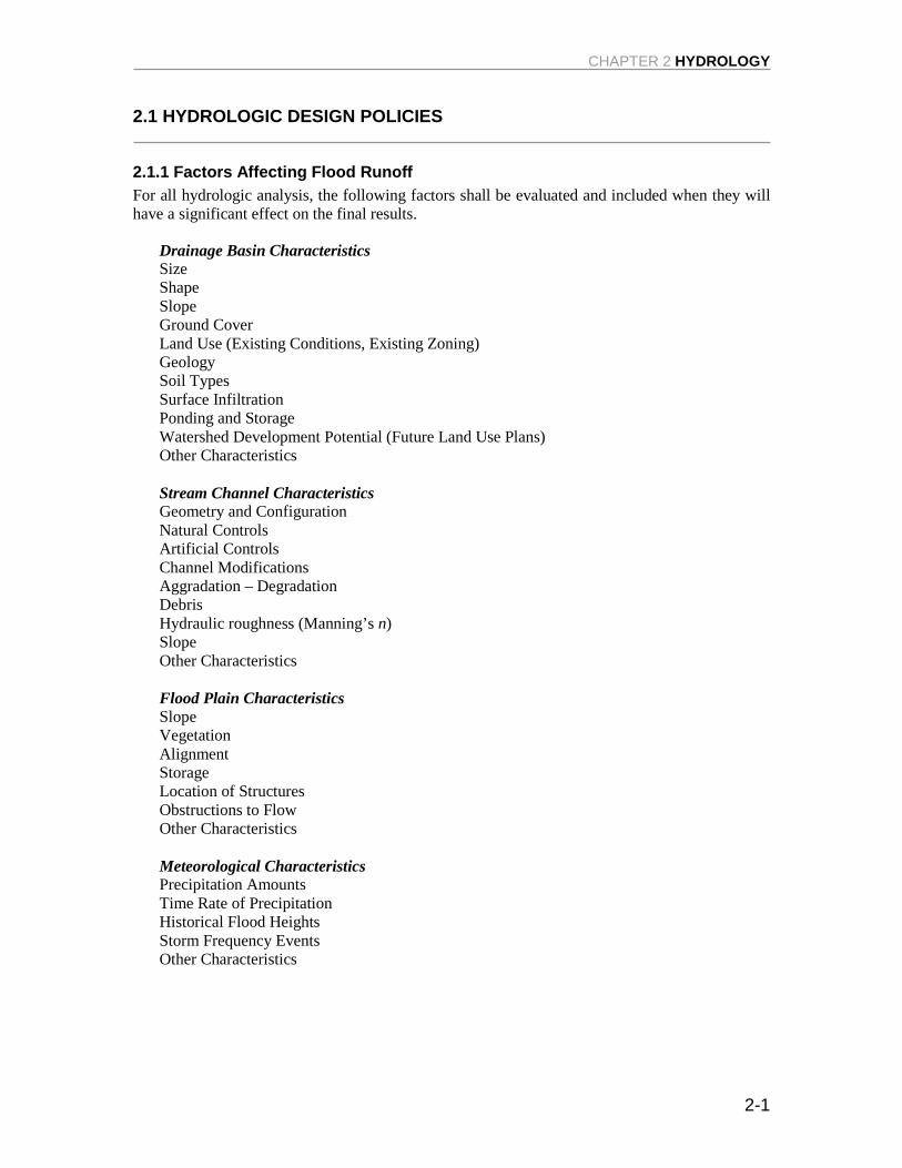
2.1 HYDROLOGIC DESIGN POLICIES
2.1.1 Factors Affecting Flood Runoff For all hydrologic analysis, the following factors shall be evaluated and included when they will have a significant effect on the final results.
Drainage Basin Characteristics Size Shape Slope Ground Cover Land Use (Existing Conditions, Existing Zoning) Geology Soil Types Surface Infiltration Ponding and Storage Watershed Development Potential (Future Land Use Plans) Other Characteristics Stream Channel Characteristics Geometry and Configuration Natural Controls Artificial Controls Channel Modifications Aggradation – Degradation Debris Hydraulic roughness (Manning’s n) Slope Other Characteristics Flood Plain Characteristics Slope Vegetation Alignment Storage Location of Structures Obstructions to Flow Other Characteristics Meteorological Characteristics Precipitation Amounts Time Rate of Precipitation Historical Flood Heights Storm Frequency Events Other Characteristics
CHARLOTTE-MECKLENBURG STORM WATER DESIGN MANUAL
2-2
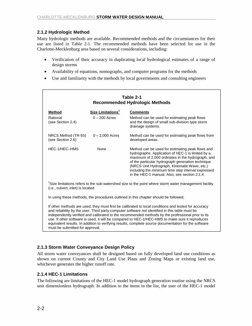
2.1.2 Hydrologic Method Many hydrologic methods are available. Recommended methods and the circumstances for their use are listed in Table 2-1. The recommended methods have been selected for use in the Charlotte-Mecklenburg area based on several considerations, including:
• Verification of their accuracy in duplicating local hydrological estimates of a range of design storms
• Availability of equations, nomographs, and computer programs for the methods • Use and familiarity with the methods by local governments and consulting engineers
Table 2-1
Recommended Hydrologic Methods
Method Size Limitations1 Comments Rational 0 – 200 Acres Method can be used for estimating peak flows (see Section 2.4) and the design of small sub-division type storm drainage systems.
NRCS Method (TR-55) 0 – 2,000 Acres Method can be used for estimating peak flows from (see Section 2.6) developed areas.
HEC-1/HEC–HMS None Method can be used for estimating peak flows and hydrographs. Application of HEC-1 is limited by a maximum of 2,000 ordinates in the hydrograph, and of the particular hydrograph generation technique (NRCS Unit Hydrograph, Kinematic Wave, etc.) including the minimum time step interval expressed in the HEC-1 manual. Also, see section 2.1.4
1Size limitations refers to the sub-watershed size to the point where storm water management facility (i.e., culvert, inlet) is located
In using these methods, the procedures outlined in this chapter should be followed.
If other methods are used, they must first be calibrated to local conditions and tested for accuracy and reliability by the user. Third party computer software not identified in this table must be independently verified and calibrated to the recommended methods by the professional prior to its use. If other software is used, it will be compared to HEC-1/HEC-HMS to make sure it reproduces equivalent results. In addition to verifying results, complete source documentation for the software must be submitted for approval.
2.1.3 Storm Water Conveyance Design Policy All storm water conveyances shall be designed based on fully developed land use conditions as shown on current County and City Land Use Plans and Zoning Maps or existing land use, whichever generates the higher runoff rate.
2.1.4 HEC-1 Limitations The following are limitations of the HEC-1 model hydrograph generation routine using the NRCS unit dimensionless hydrograph. In addition to the items in the list, the user of the HEC-1 model
CHAPTER 2 HYDROLOGY
2-3
must be knowledgeable of the limitations of the hydrologic and hydraulic methodologies which are being applied by the model.
• The computation interval must not be significantly less than the minimum rainfall increment on the “PH” record, otherwise a portion of the rainfall is lost because the program cannot perform the logarithmic interpolation necessary for the development of the complete hyetograph. Standard HEC-1 model input uses a 5-minute “worst” precipitation increment. Therefore, the model may not be used with a computation interval less than 5 minutes unless the rainfall hyetograph is input with “PC” or “PI” records. The computation interval, when multiplied by the number of hydrograph ordinates, must also be greater than the storm duration which is planned to be studied (6 hour, 24 hour, etc.). Not having the program set to allow the storm to run causes hydrographs to be inappropriately peaked due to the lack of necessary time to fit in the needed runoff hydrograph.
• The NRCS unit dimensionless hydrograph may not be used when the computation interval is greater than 0.29 times the lag time of the watershed. This limitation translates into a minimum time of concentration of 5.75 minutes which typically occurs in watersheds of 3 acres or less. The result of exceeding this limitation is that the resulting hydrograph may underestimate the peak flow by computing the peak flow values on either side of the peak of the hydrograph. However, the volume under the resulting hydrograph is correct and all volume computation such as detention storage is correct.
2.2 HYDROLOGIC ANALYSIS PROCEDURE FLOWCHART
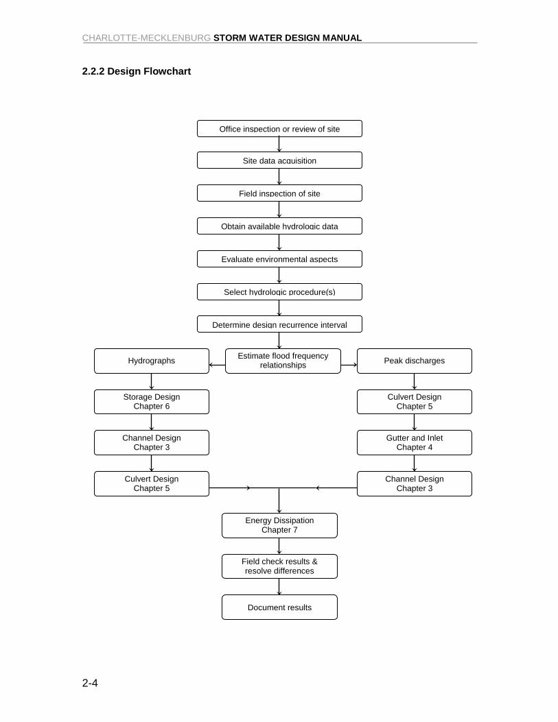
2.2.1 Purpose and Use The purpose of the hydrologic analysis procedure flowchart is to show the steps or elements which need to be completed for the hydrologic analysis, and the different designs that will use the hydrologic estimates.
CHARLOTTE-MECKLENBURG STORM WATER DESIGN MANUAL
2-4
Office inspection or review of site
Site data acquisition
Field inspection of site
Obtain available hydrologic data
Evaluate environmental aspects
Select hydrologic procedure(s)
Determine design recurrence interval
Energy Dissipation Chapter 7
Field check results & resolve differences
Document results
2.2.2 Design Flowchart
Estimate flood frequency relationships Hydrographs Peak discharges
Storage Design Chapter 6
Culvert Design Chapter 5
Channel Design Chapter 3
Gutter and Inlet Chapter 4
Culvert Design Chapter 5
Channel Design Chapter 3
CHAPTER 2 HYDROLOGY
2-5
2.3 DESIGN FREQUENCY
2.3.1 Design Frequencies Description Design Storm
Storm system pipes 10 year Ditch systems 10 year Culverts/Cross-drain (subdivision streets) 25 year Culverts/Cross-drain (thoroughfare roads) 50 year Culverts (over regulated floodways) 100 year Culverts/Cross-drain (primary access streets) No overtopping in 100 year Usable and functionable part of structure or building 100 year + 1 foot (as defined in the Subdivision Ordinance)
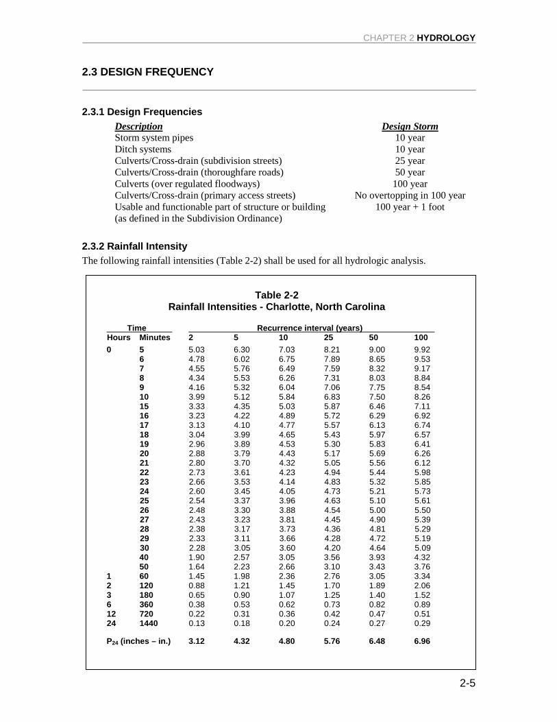
2.3.2 Rainfall Intensity The following rainfall intensities (Table 2-2) shall be used for all hydrologic analysis.
Table 2-2 Rainfall Intensities - Charlotte, North Carolina
Time Recurrence interval (years) Hours Minutes 2 5 10 25 50 100 0 5 5.03 6.30 7.03 8.21 9.00 9.92 6 4.78 6.02 6.75 7.89 8.65 9.53 7 4.55 5.76 6.49 7.59 8.32 9.17 8 4.34 5.53 6.26 7.31 8.03 8.84 9 4.16 5.32 6.04 7.06 7.75 8.54 10 3.99 5.12 5.84 6.83 7.50 8.26 15 3.33 4.35 5.03 5.87 6.46 7.11 16 3.23 4.22 4.89 5.72 6.29 6.92 17 3.13 4.10 4.77 5.57 6.13 6.74 18 3.04 3.99 4.65 5.43 5.97 6.57 19 2.96 3.89 4.53 5.30 5.83 6.41 20 2.88 3.79 4.43 5.17 5.69 6.26 21 2.80 3.70 4.32 5.05 5.56 6.12 22 2.73 3.61 4.23 4.94 5.44 5.98 23 2.66 3.53 4.14 4.83 5.32 5.85 24 2.60 3.45 4.05 4.73 5.21 5.73 25 2.54 3.37 3.96 4.63 5.10 5.61 26 2.48 3.30 3.88 4.54 5.00 5.50 27 2.43 3.23 3.81 4.45 4.90 5.39 28 2.38 3.17 3.73 4.36 4.81 5.29 29 2.33 3.11 3.66 4.28 4.72 5.19 30 2.28 3.05 3.60 4.20 4.64 5.09 40 1.90 2.57 3.05 3.56 3.93 4.32 50 1.64 2.23 2.66 3.10 3.43 3.76
1 60 1.45 1.98 2.36 2.76 3.05 3.34 2 120 0.88 1.21 1.45 1.70 1.89 2.06 3 180 0.65 0.90 1.07 1.25 1.40 1.52 6 360 0.38 0.53 0.62 0.73 0.82 0.89 12 720 0.22 0.31 0.36 0.42 0.47 0.51 24 1440 0.13 0.18 0.20 0.24 0.27 0.29
P24 (inches – in.) 3.12 4.32 4.80 5.76 6.48 6.96
CHARLOTTE-MECKLENBURG STORM WATER DESIGN MANUAL
2-6
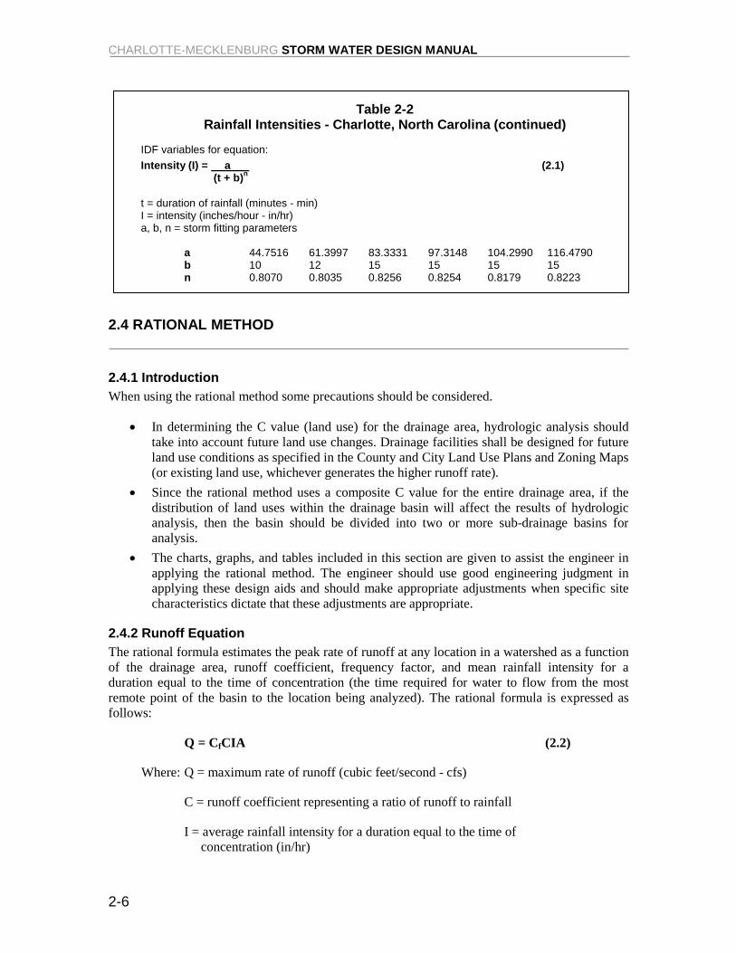
Table 2-2
Rainfall Intensities - Charlotte, North Carolina (continued) IDF variables for equation: Intensity (I) = a (2.1) (t + b)n t = duration of rainfall (minutes - min) I = intensity (inches/hour - in/hr) a, b, n = storm fitting parameters a 44.7516 61.3997 83.3331 97.3148 104.2990 116.4790 b 10 12 15 15 15 15 n 0.8070 0.8035 0.8256 0.8254 0.8179 0.8223
2.4 RATIONAL METHOD
2.4.1 Introduction When using the rational method some precautions should be considered.
• In determining the C value (land use) for the drainage area, hydrologic analysis should take into account future land use changes. Drainage facilities shall be designed for future land use conditions as specified in the County and City Land Use Plans and Zoning Maps (or existing land use, whichever generates the higher runoff rate).
• Since the rational method uses a composite C value for the entire drainage area, if the distribution of land uses within the drainage basin will affect the results of hydrologic analysis, then the basin should be divided into two or more sub-drainage basins for analysis.
• The charts, graphs, and tables included in this section are given to assist the engineer in applying the rational method. The engineer should use good engineering judgment in applying these design aids and should make appropriate adjustments when specific site characteristics dictate that these adjustments are appropriate.
2.4.2 Runoff Equation The rational formula estimates the peak rate of runoff at any location in a watershed as a function of the drainage area, runoff coefficient, frequency factor, and mean rainfall intensity for a duration equal to the time of concentration (the time required for water to flow from the most remote point of the basin to the location being analyzed). The rational formula is expressed as follows:
Q = CfCIA (2.2)
Where: Q = maximum rate of runoff (cubic feet/second - cfs)
C = runoff coefficient representing a ratio of runoff to rainfall
I = average rainfall intensity for a duration equal to the time of concentration (in/hr)
CHAPTER 2 HYDROLOGY
2-7
A = drainage area contributing to the design point location (acres)
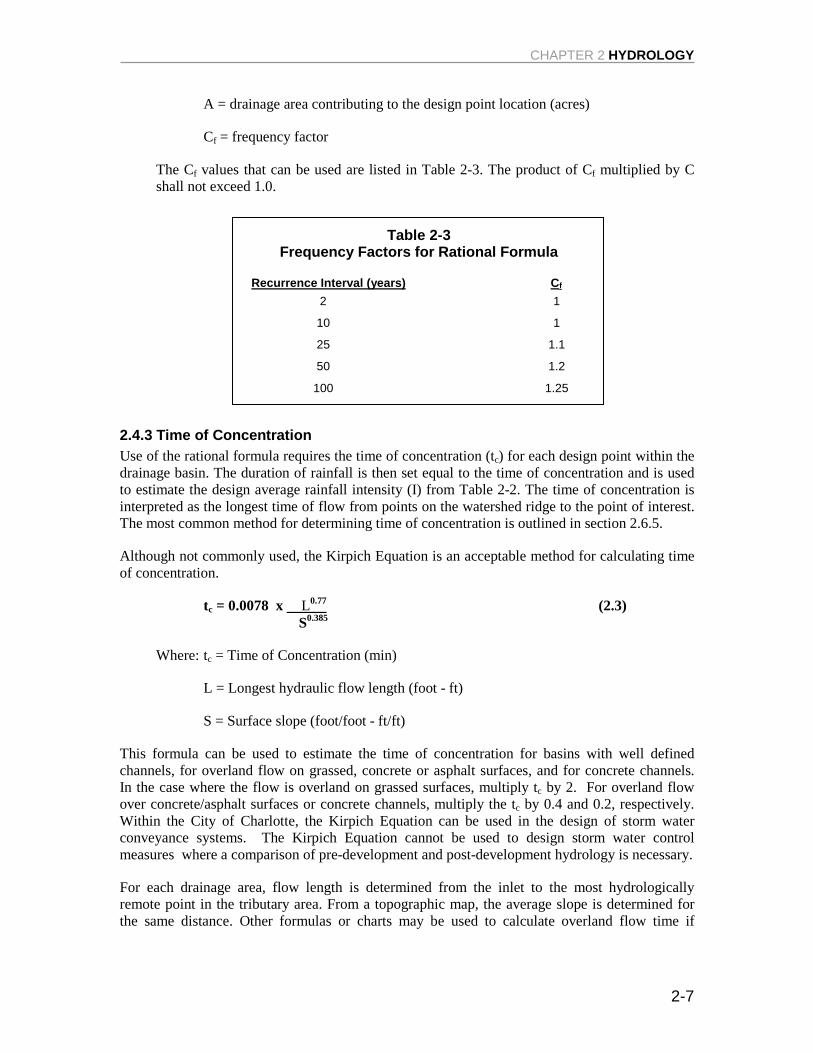
Cf = frequency factor
The Cf values that can be used are listed in Table 2-3. The product of Cf multiplied by C shall not exceed 1.0.
Table 2-3 Frequency Factors for Rational Formula
Recurrence Interval (years) Cf 2 1
10 1
25 1.1
50 1.2
100 1.25
2.4.3 Time of Concentration Use of the rational formula requires the time of concentration (tc) for each design point within the drainage basin. The duration of rainfall is then set equal to the time of concentration and is used to estimate the design average rainfall intensity (I) from Table 2-2. The time of concentration is interpreted as the longest time of flow from points on the watershed ridge to the point of interest. The most common method for determining time of concentration is outlined in section 2.6.5.
Although not commonly used, the Kirpich Equation is an acceptable method for calculating time of concentration.
tc = 0.0078 x L0.77 (2.3) S0.385
Where: tc = Time of Concentration (min)
L = Longest hydraulic flow length (foot - ft)
S = Surface slope (foot/foot - ft/ft)
This formula can be used to estimate the time of concentration for basins with well defined channels, for overland flow on grassed, concrete or asphalt surfaces, and for concrete channels. In the case where the flow is overland on grassed surfaces, multiply tc by 2. For overland flow over concrete/asphalt surfaces or concrete channels, multiply the tc by 0.4 and 0.2, respectively. Within the City of Charlotte, the Kirpich Equation can be used in the design of storm water conveyance systems. The Kirpich Equation cannot be used to design storm water control measures where a comparison of pre-development and post-development hydrology is necessary.
For each drainage area, flow length is determined from the inlet to the most hydrologically remote point in the tributary area. From a topographic map, the average slope is determined for the same distance. Other formulas or charts may be used to calculate overland flow time if
CHARLOTTE-MECKLENBURG STORM WATER DESIGN MANUAL
2-8
approved by the City/County Engineering Departments. Note: time of concentration cannot be less than 5 minutes.
A common error should be avoided when calculating tc. In some cases runoff from a portion of the drainage area which is highly impervious may result in a greater peak discharge than would occur if the entire area were considered. In these cases, adjustments can be made to the drainage area by disregarding those areas where flow time is too slow to add to the peak discharge.
2.4.4 Rainfall Intensity The rainfall intensity (I) is the average rainfall rate in inches/hour for a duration equal to the time of concentration for a selected return period. Once a particular return period has been selected for design and a time of concentration calculated for the drainage area, the rainfall intensity can be determined from Rainfall-Intensity-Duration data given in Table 2-2. Straight-line interpolation can be used to obtain rainfall intensity values for storm durations between the values given in Table 2-2.
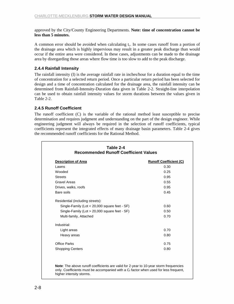
2.4.5 Runoff Coefficient The runoff coefficient (C) is the variable of the rational method least susceptible to precise determination and requires judgment and understanding on the part of the design engineer. While engineering judgment will always be required in the selection of runoff coefficients, typical coefficients represent the integrated effects of many drainage basin parameters. Table 2-4 gives the recommended runoff coefficients for the Rational Method.
Table 2-4 Recommended Runoff Coefficient Values
Description of Area Runoff Coefficient (C) Lawns 0.30 Wooded 0.25 Streets 0.95 Gravel Areas 0.55 Drives, walks, roofs 0.95 Bare soils 0.45
Residential (including streets): Single-Family (Lot < 20,000 square feet - SF) 0.60 Single-Family (Lot > 20,000 square feet - SF) 0.50 Multi-family, Attached 0.70
Industrial: Light areas 0.70 Heavy areas 0.80
Office Parks 0.75 Shopping Centers 0.80
Note: The above runoff coefficients are valid for 2-year to 10-year storm frequencies only. Coefficients must be accompanied with a Cf factor when used for less frequent, higher intensity storms.
CHAPTER 2 HYDROLOGY
2-9
2.4.6 Composite Coefficients It is often desirable to develop a composite runoff coefficient based on the percentage of different types of surfaces in the drainage areas. Composites can be made with the values from Table 2-4 by using percentages of different land uses. The composite procedure can be applied to an entire drainage area or to typical “sample” blocks as a guide to selection of reasonable values of the coefficient for an entire area.
It should be remembered that the rational method assumes that all land uses within a drainage area are uniformly distributed throughout the area. If it is important to locate a specific land use within the drainage area then another hydrologic method should be used where hydrographs can be generated and routed through the drainage area.
2.5 EXAMPLE PROBLEM - RATIONAL METHOD
Introduction Following is an example problem which illustrates the application of the Rational Method to estimate peak discharges.
Problem Preliminary estimates of the maximum rate of runoff are needed at the inlet to a culvert for a 25-year and 100-year return period.
Site Data From a topographic map field survey, the area of the drainage basin upstream from the point in question is found to be 18 acres. In addition the following data were measured:
Flow Path Average slope = 2.0% Length of flow in well defined channel = 1,000 ft
Land Use From existing land use maps, land use for the drainage basin was estimated to be:
Single Family (< 20,000 SF) 80% Light Industrial 20%
Time of Concentration Since this problem involves determining the flows for a storm water conveyance system, utilization of the conservative and simplistic Kirpich method may be appropriate: Using Equation 2.3 with a flow length of 1,000 ft and slope of 2.0%
tc = 0.0078 x 1,0000.77 = 7.2 minutes 0.020.385
Rainfall Intensity From Table 2-2, with a duration equal to 7.2 minutes, the intensity can be selected by interpolation.
CHARLOTTE-MECKLENBURG STORM WATER DESIGN MANUAL
2-10
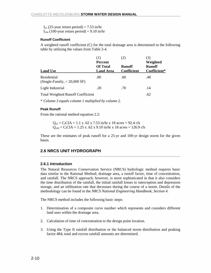
I25 (25-year return period) = 7.53 in/hr I100 (100-year return period) = 9.10 in/hr
Runoff Coefficient A weighted runoff coefficient (C) for the total drainage area is determined in the following table by utilizing the values from Table 2-4.
(1) (2) (3) Percent Weighted Of Total Runoff Runoff Land Use Land Area Coefficient Coefficient*
Residential .80 .60 .48 (Single-Family, < 20,000 SF)
Light Industrial .20 .70 .14
Total Weighted Runoff Coefficient .62
* Column 3 equals column 1 multiplied by column 2.
Peak Runoff From the rational method equation 2.2:
Q25 = CfCIA = 1.1 x .62 x 7.53 in/hr x 18 acres = 92.4 cfs Q100 = CfCIA = 1.25 x .62 x 9.10 in/hr x 18 acres = 126.9 cfs
These are the estimates of peak runoff for a 25-yr and 100-yr design storm for the given basin.
2.6 NRCS UNIT HYDROGRAPH
2.6.1 Introduction The Natural Resources Conservation Service (NRCS) hydrologic method requires basic data similar to the Rational Method; drainage area, a runoff factor, time of concentration, and rainfall. The NRCS approach; however, is more sophisticated in that it also considers the time distribution of the rainfall, the initial rainfall losses to interception and depression storage, and an infiltration rate that decreases during the course of a storm. Details of the methodology can be found in the NRCS National Engineering Handbook, Section 4.
The NRCS method includes the following basic steps:
1. Determination of a composite curve number which represents and considers different land uses within the drainage area.
2. Calculation of time of concentration to the design point location.
3. Using the Type II rainfall distribution or the balanced storm distribution and peaking factor 484, total and excess rainfall amounts are determined.
CHAPTER 2 HYDROLOGY
2-11
4. Using the unit hydrograph approach, triangular and composite hydrographs are developed for the drainage area.
2.6.2 Equations and Concepts The following discussion outlines the equation and basic concepts utilized in the NRCS method.
Drainage Area—the drainage area of a watershed is determined from topographic maps and field surveys. For large drainage areas it might be necessary to divide the area into sub-drainage areas to account for major land use changes, obtain analysis results at different points within drainage area, and route flows to design study points of interest.
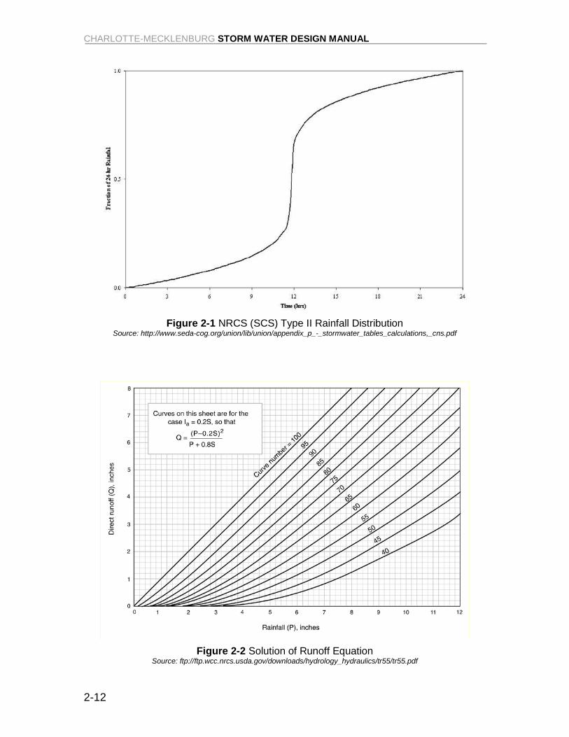
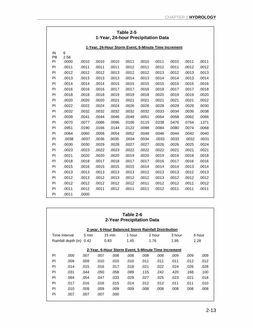
Rainfall—The NRCS method applicable to the Charlotte-Mecklenburg area is based on a storm event which has a Type II time distribution. For example, the one-year 24-hour storm event is based on the distribution shown in Figure 2-1. Tables 2-5 through 2-10 show a center weighted balanced distribution for various 6-hour storm events to be used for the Charlotte-Mecklenburg area.
Rainfall-Runoff Equation—A relationship between accumulated rainfall and accumulated runoff was derived by NRCS from experimental plots for numerous soils and vegetative cover conditions. The following NRCS runoff equation is used to estimate direct runoff from 24-hour or 1-day storm rainfall. The equation is:
Q = (P – Ia)2 (2.4) (P – Ia) + S
Where: Q = accumulated direct runoff (inches) P = accumulated rainfall or potential maximum runoff (inches) Ia = initial abstraction including surface storage, interception, and infiltration
prior to runoff (inches) S = potential maximum soil retention (inches)
The empirical relationship used in the NRCS runoff equation for estimating Ia is :
Ia = 0.2S (2.5)
Substituting 0.2S for Ia in equation 2.4, the NRCS rainfall-runoff equation becomes:
Q = (P – 0.2S)2 (2.6) (P + 0.8S)
Where: S = (1,000/CN) – 10 CN = NRCS curve number (see section 2.6.3)
Figure 2-2 shows a graphical solution of this equation which enables the precipitation excess from a storm to be obtained if the total rainfall and watershed curve number are known. For example, 4.1 inches of direct runoff would result if 5.8 inches of rainfall occurs on a watershed with a curve number of 85.
CHARLOTTE-MECKLENBURG STORM WATER DESIGN MANUAL
2-12
Figure 2-1 NRCS (SCS) Type II Rainfall Distribution
Source: http://www.seda-cog.org/union/lib/union/appendix_p_-_stormwater_tables_calculations,_cns.pdf
Figure 2-2 Solution of Runoff Equation
Source: ftp://ftp.wcc.nrcs.usda.gov/downloads/hydrology_hydraulics/tr55/tr55.pdf
CHAPTER 2 HYDROLOGY
2-13
Table 2-5 1-Year, 24-hour Precipitation Data
1-Year, 24-Hour Storm Event, 6-Minute Time Increment IN 6 PB 2.58 PI .0000 .0010 .0010 .0010 .0011 .0010 .0011 .0010 .0011 .0011 PI .0011 .0011 .0011 .0011 .0012 .0011 .0012 .0011 .0012 .0012 PI .0012 .0012 .0012 .0013 .0012 .0012 .0013 .0012 .0013 .0013 PI .0013 .0013 .0013 .0013 .0014 .0013 .0014 .0014 .0013 .0014 PI .0014 .0014 .0014 .0015 .0015 .0015 .0015 .0015 .0015 .0016 PI .0016 .0016 .0016 .0017 .0017 .0016 .0018 .0017 .0017 .0018 PI .0018 .0018 .0018 .0019 .0019 .0018 .0020 .0019 .0019 .0020 PI .0020 .0020 .0020 .0021 .0021 .0021 .0021 .0021 .0021 .0022 PI .0022 .0022 .0024 .0024 .0026 .0026 .0028 .0029 .0029 .0030 PI .0032 .0032 .0032 .0032 .0032 .0032 .0033 .0034 .0036 .0038 PI .0039 .0041 .0044 .0046 .0048 .0051 .0054 .0058 .0062 .0066 PI .0070 .0077 .0086 .0096 .0106 .0115 .0238 .0476 .0764 .1371 PI .0951 .0190 .0166 .0144 .0122 .0098 .0084 .0080 .0074 .0068 PI .0064 .0060 .0056 .0054 .0052 .0048 .0046 .0044 .0042 .0040 PI .0038 .0037 .0036 .0035 .0034 .0034 .0033 .0033 .0032 .0031 PI .0030 .0030 .0029 .0028 .0027 .0027 .0026 .0026 .0025 .0024 PI .0023 .0023 .0022 .0023 .0022 .0022 .0022 .0021 .0021 .0021 PI .0021 .0020 .0020 .0020 .0019 .0020 .0019 .0019 .0018 .0018 PI .0018 .0018 .0017 .0018 .0017 .0017 .0016 .0017 .0016 .0016 PI .0015 .0016 .0015 .0015 .0015 .0014 .0014 .0014 .0013 .0014 PI .0013 .0013 .0013 .0013 .0013 .0012 .0013 .0013 .0012 .0013 PI .0012 .0013 .0012 .0013 .0012 .0012 .0013 .0012 .0012 .0012 PI .0012 .0012 .0012 .0012 .0012 .0011 .0012 .0012 .0011 .0012 PI .0011 .0012 .0011 .0012 .0011 .0011 .0012 .0011 .0011 .0011 PI .0011 .0000
Table 2-6
2-Year Precipitation Data
2-year, 6-Hour Balanced Storm Rainfall Distribution Time Interval 5 min 15 min 1 hour 2 hour 3 hour 6 hour Rainfall depth (in) 0.42 0.83 1.45 1.76 1.95 2.28
2-Year, 6-Hour Storm Event, 5-Minute Time Increment PI .000 .007 .007 .008 .008 .008 .008 .009 .009 .009 PI .009 .009 .010 .010 .010 .011 .011 .011 .012 .012 PI .014 .015 .016 .017 .018 .021 .022 .024 .026 .028 PI .031 .044 .050 .058 .089 .115 .242 .420 .168 .100 PI .064 ,054 .047 .033 .029 .027 .025 .023 .021 .018 PI .017 .016 .016 .015 .014 .012 .012 .011 .011 .010 PI .010 .009 .009 .009 .009 .008 .008 .008 .008 .008 PI .007 .007 .007 .000
CHARLOTTE-MECKLENBURG STORM WATER DESIGN MANUAL
2-14
Table 2-7 10-Year Precipitation Data
10-Year, 6-Hour Balanced Storm Rainfall Distribution Time Interval 5 min 15 min 1 hour 2 hour 3 hour 6 hour Rainfall depth (in) 0.59 1.26 2.36 2.90 3.21 3.72
10-Year, 6-Hour Storm Event, 5-Minute Time Increment PI .000 .011 .011 .011 .012 .012 .012 .013 .013 .013 PI .014 .014 .015 .015 .016 .016 .017 .018 .018 .023 PI .024 .025 .026 .027 .029 .036 .039 .042 .045 .049 PI .054 .079 .089 .103 .161 .201 .395 .590 .275 .177 PI .112 .095 .084 .057 .051 .047 .043 .040 .038 .030 PI .028 .027 .025 .024 .023 .019 .018 .017 .017 .016 PI .016 .015 .015 .014 .014 .013 .013 .012 .012 .012 PI .011 .011 .011 .000
Table 2-8 25-Year Precipitation Data
25-Year, 6-Hour Balanced Storm Rainfall Distribution Time Interval 5 min 15 min 1 hour 2 hour 3 hour 6 hour Rainfall depth (in) 0.68 1.47 2.76 3.40 3.75 4.38
25-Year, 6-Hour Storm Event, 5-Minute Time Increment PI .000 .014 .014 .015 .015 .015 .016 .016 .016 .017 PI .017 .018 .019 .019 .020 .020 .022 .022 .023 .026 PI .027 .028 .029 .031 .033 .043 .046 .049 .053 .058 PI .064 .093 .104 .120 .188 .234 .461 .680 .321 .207 PI .131 .112 .098 .067 .061 .056 .051 .048 .045 .034 PI .032 .030 .029 .027 .026 .023 .022 .021 .021 .020 PI .019 .019 .018 .017 .017 .017 .017 .016 .015 .015 PI .015 .014 .014 .000
CHAPTER 2 HYDROLOGY
2-15
Table 2-9 50-Year Precipitation Data
50-Year, 6-Hour Balanced Storm Rainfall Distribution Time Interval 5 min 15 min 1 hour 2 hour 3 hour 6 hour Rainfall depth (in) 0.75 1.62 3.05 3.78 4.20 4.92
50-Year, 6-Hour Storm Event, 5-minute Time Increment PI .000 .016 .016 .016 .017 .018 .018 .019 .019 .019 PI .020 .020 .021 .022 .022 .023 .024 .025 .026 .031 PI .032 .034 .035 .037 .039 .050 .053 .056 .061 .066 PI .073 .103 .116 .134 .208 .259 .508 .750 .354 .229 PI .146 .124 .109 .077 .069 .063 .059 .055 .051 .040 PI .038 .036 .034 .033 .031 .026 .025 .024 .024 .023 PI .022 .021 .021 .020 .020 .019 .019 .018 .018 .017 PI .017 .016 .016 .000
Table 2-10 100-Year Precipitation Data
100-Year, 6-Hour Balanced Storm Rainfall Distribution Time Interval 5 min 15 min 1 hour 2 hour 3 hour 6 hour Rainfall depth (in) 0.83 1.77 3.34 4.12 4.56 5.34
100-Year, 6-Hour Storm Event, 5-Minute Time Increment PI .000 .017 .017 .018 .018 .019 .020 .020 .020 .021 PI .022 .022 .023 .023 .024 .025 .026 .027 .028 .032 PI .034 .035 .037 .039 .041 .053 .056 .060 .065 .071 PI .078 .113 .126 .147 .226 .282 .555 .830 .386 .250 PI .160 .136 .119 .082 .074 .068 .063 .058 .055 .042 PI .040 .038 .036 .034 .033 .029 .027 .026 .025 .025 PI .024 .023 .022 .022 .021 .021 .020 .020 .019 .019 PI .018 .018 .017 .000
CHARLOTTE-MECKLENBURG STORM WATER DESIGN MANUAL
2-16
2.6.3 Runoff Factor The principal physical watershed characteristics affecting the relationship between rainfall and runoff are land use, land cover, soil types and land slope. The NRCS uses a combination of soil conditions and land-use (ground cover) to assign a runoff factor to an area. These runoff factors, called runoff curve numbers (CN), indicate the runoff potential of an area. The higher the CN, the higher is the runoff potential.
Soil properties influence the relationship between runoff and rainfall since soils have differing rates of infiltration. Based on infiltration rates, the NRCS has divided soils into four hydrologic soil groups as follows:
Group A - Soils having a low runoff potential due to high infiltration rates. These soils consist primarily of deep, well drained sand and gravels.
Group B - Soils having a moderately low runoff potential due to moderate infiltration rates. These soils consist primarily of moderately deep to deep, moderately well to well drained soils with moderately fine to moderately coarse textures.
Group C - Soils having moderately high runoff potential due to slow infiltration rates. These soils consist primarily of soils in which a layer exists near the surface that impedes the downward movement of water of soils with moderately fine to fine texture.
Group D - Soils having a high runoff potential due to very slow infiltration rates. These soils consist primarily of clays with high swelling potential, soils with permanently high water tables, soils with a claypan or clay layer at or near the surface, and shallow soils over nearly impervious parent material.
A list of soils for Charlotte and Mecklenburg County and their hydrologic classifications are presented in Table 2-11 below. Soil survey maps can be obtained from local NRCS offices.
Table 2-11 Hydrologic Soil Groups for Charlotte-Mecklenburg
Series Hydrologic Series Hydrologic Name Group Name Group Appling B Lignum C Cecil B Mecklenburg C Davidson B Monacan C Enon C Pacolet B Georgeville B Pits D Goldston C Vance C Helena C Wilkes C Iredell D
Consideration should be given to the effects of soil compaction due to development on the natural hydrologic soil group. If heavy equipment can be expected to compact the soil during construction or if grading will mix the surface and subsurface soils, appropriate changes should be made in the soil group selected. Also, runoff curve numbers vary with
CHAPTER 2 HYDROLOGY
2-17
the antecedent soil moisture conditions. Average antecedent soil moisture conditions (AMC II) are recommended for all hydrologic analysis.
Table 2-12 gives recommended curve number values for a range of different land uses.
2.6.4 Modifications for Developed Conditions Several factors, such as the percentage of impervious area and the means of conveying runoff from impervious areas to the drainage system, should be considered in computing CN for developed areas. For example, consider whether the impervious areas connect directly to the drainage system, or to lawns or other pervious areas where infiltration can occur.
The curve number values given in Table 2-12 on the following page are based on directly connected impervious area. An impervious area is considered directly connected if runoff from it flows directly into the drainage system. It is also considered directly connected if runoff from it occurs as concentrated shallow flow that runs over a pervious area and then into a drainage system.
It is possible that curve number values from developed areas could be reduced by not directly connecting impervious surfaces to the drainage system. For a discussion of connected and unconnected impervious areas and their effect on curve number values see Appendix A at the end of this chapter.
CHARLOTTE-MECKLENBURG STORM WATER DESIGN MANUAL
2-18
Table 2-12 Runoff Curve Numbers1
Curve numbers for ------------------------------Cover description -------------------------------- -----hydrologic soil group----- Average percent Cover type and hydrologic condition impervious area 2/ A B C D
Fully developed urban areas (vegetation established)
Open space (lawns, parks, golf courses, cemeteries, etc.) 3/: Poor condition (grass cover < 50%) ............................ 68 79 86 89 Fair condition (grass cover 50% to 75%) .................... 49 69 79 84 Good condition (grass cover > 75%) ........................... 39 61 74 80 Impervious areas: Paved parking lots, roofs, driveways, etc. (excluding right-of-way) ..................................... 98 98 98 98 Streets and roads: Paved; curbs and storm sewers (excluding right-of-way) ....................................................... 98 98 98 98 Paved; open ditches (including right-of-way) .... 83 89 92 93 Gravel (including right-of-way) .......................... 76 85 89 91 Dirt (including right-of-way) .............................. 72 82 87 89 Urban districts: Commercial and business ............................................ 85 89 92 94 95 Industrial ..................................................................... 72 81 88 91 93 Residential districts by average lot size: 1/8 acre or less (town houses) ..................................... 65 77 85 90 92 1/4 acre ........................................................................ 38 61 75 83 87 1/3 acre ........................................................................ 30 57 72 81 86 1/2 acre ........................................................................ 25 54 70 80 85 1 acre ........................................................................... 20 51 68 79 84 2 acres ......................................................................... 12 46 65 77 82 Agricultural Lands Pasture, grassland or range (continuous for age for grazing)4 Poor hydrologic condition ........................................... 68 79 86 89 Fair hydrologic condition ............................................ 49 69 79 84 Good hydrologic condition ......................................... 39 61 74 80 Woods Poor hydrologic condition ........................................... 45 66 77 83 Fair hydrologic condition ............................................ 36 60 73 79 Good hydrologic condition ......................................... 30 55 70 77 Developing urban areas Newly graded areas (pervious areas only, no vegetation) ........................... 77 86 91 94
1 Average runoff condition, and Ia = 0.2S. 2 The average percent impervious area shown was used to develop the composite CN’s. Other assumptions are as follows: impervious areas
area directly connected to the drainage system, impervious areas have a CN of 98, and pervious areas are considered equivalent to open space in good hydrologic condition.
3 CN’s shown are equivalent to those of pasture. Composite CN’s may be computed for other combinations of open space cover type. 4 Poor: Forest litter, small trees, and brush are destroyed by heavy grazing or regular burning. Fair: Woods are grazed but not burned, and some forest litter covers the soil. Good: Woods are protected from grazing, and litter and brush adequately cover the soil.
Source: 210-VI-TR-55, Second Edition, June 1986
CHAPTER 2 HYDROLOGY
2-19
2.6.5 Travel Time Estimation Travel time (Tt ) is the time it takes water to travel from one location to another within a watershed through the various components of the drainage system. Time of concentration (tc) is computed by summing all the travel times of consecutive components of the drainage conveyance system from the hydraulically most distant point of the watershed to the point of interest within the watershed.
Following is a discussion of related procedures and equations.
2.6.5.1 Travel Time Water moves through a watershed as sheet flow, shallow concentrated flow, open channel, or some combination of these. The type that occurs is a function of the conveyance system and is best determined by field inspection.
Travel time is the ratio of flow length to flow velocity:
Tt = L x 0.0167 (2.7) V
Where: Tt = travel time (min) L = flow length (ft) V = average velocity (feet/second - ft/s)
2.6.5.2 Time of Concentration The time of concentration is the sum of Tt values for the various consecutive flow segments along the path extending from the hydraulically most distant point in the watershed to the point of interest.
tc = Tt1 + Tt2 … Tn (2.8)
Where: tc = time of concentration (hour - hr) n = number of flow segments
2.6.5.3 Sheet Flow Sheet flow is flow over plane surfaces. It occurs in the headwater of streams. With sheet flow, the friction value (Manning’s n) is an effective roughness coefficient that includes the effect of raindrop impact; drag over the plane surface; obstacles such as litter, crop ridges, and rocks; and erosion and transportation of sediment. These n values are for very shallow flow depths of about 0.1 foot or so. Also please note, when designing a drainage system, the sheet flow path is not necessarily the same before and after development and grading operations have been completed. Selecting sheet flow paths in excess of 100 feet in developed areas and 300 feet in undeveloped areas should be done only after careful consideration.
For sheet flow less than 300 feet in undeveloped areas and less than 100 ft in developed areas use Manning’s kinematic solution (Overton and Meadows 1976) to compute Tt:
Tt = 0.42 (nL)0.8 (2.9) (P2)1/2(S)0.4
CHARLOTTE-MECKLENBURG STORM WATER DESIGN MANUAL
2-20
Where: Tt = travel time (min) n = Manning’s roughness coefficient, reference Table 2-13 L = flow length (ft) P2 = 2-year, 24 hour rainfall = 3.12 inches S = slope of hydraulic grade line (land slope – ft/ft)
Substituting the constant rainfall amount the travel equation becomes:
Tt = 0.238 (nL)0.8 (2.10) (S)0.4
Thus the final equations for paved and unpaved areas are:
Paved Tt = 0.0065 [(L)0.8 / (S)0.4] (2.11) (n = .011) V = 2.56(S)0.4(L)0.2 (2.12)
Unpaved Tt = 0.076 [ (L)0.8 / (S)0.4 ] (2.13) (n = .24) V = 0.22(S)0.4(L)0.2 (2.14)
Where: V = Velocity (ft/s) Tt = Travel time (min)
CHAPTER 2 HYDROLOGY
2-21
Table 2-13 Roughness Coefficients (Manning’s n)1 for Sheet Flow
Surface Description n Smooth surfaces (concrete, asphalt, 0.011
gravel, or bare soil)
Fallow (no residue) 0.05
Cultivated Soils: Residue Cover < 20% 0.06 Residue Cover > 20% 0.17
Grass: Short grass prairie 0.15 Dense grasses2 0.24 Bermuda grass 0.41
Range (natural) 0.13
Woods3 Light underbrush 0.40 Dense underbrush 0.80
1The n values are a composite of information by Engman (1986). 2Includes species such as weeping lovegrass, bluegrass, buffalo grass, blue gamma grass, and native grass mixture. 3When selecting n, consider cover to a height of about 0.1 ft. This is the only part of the plant cover that will obstruct sheet flow. Source: NRCS, TR-55, Second Edition, June 1986
2.6.5.4 Shallow Concentrated Flow After a maximum of 300 feet in undeveloped areas or 100 feet in developed areas, sheet flow usually becomes shallow concentrated flow. Average velocities for estimating travel time for shallow concentrated flow can be computed using the following equations. These equations can also be used for slopes less than 0.005 ft/ft.
Unpaved V = 16.1345(S)1/2 (2.15)
Paved V = 20.3282(S)1/2 (2.16)
Where: V = average velocity (ft/s) S = slope of hydraulic grade line (watercourse, slope, ft/ft)
These two equations are based on the solution of Manning’s equation with different assumptions for n (Manning’s roughness coefficient) and r (hydraulic radius, ft). For unpaved areas, n is 0.05 and r is 0.4; for paved areas, n is 0.025 and r is 0.2.
After determining average velocity using equations 2.15 or 2.16, use equation 2.7 to estimate travel time for the shallow concentrated flow segment.
CHARLOTTE-MECKLENBURG STORM WATER DESIGN MANUAL
2-22
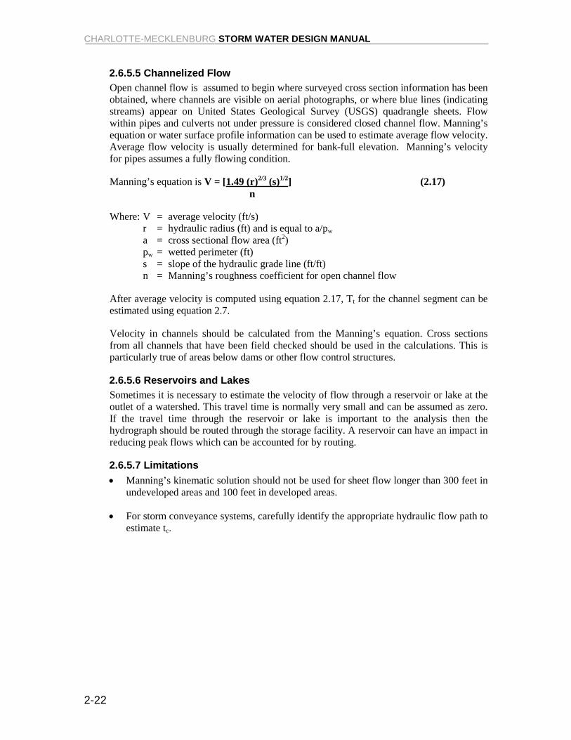
2.6.5.5 Channelized Flow Open channel flow is assumed to begin where surveyed cross section information has been obtained, where channels are visible on aerial photographs, or where blue lines (indicating streams) appear on United States Geological Survey (USGS) quadrangle sheets. Flow within pipes and culverts not under pressure is considered closed channel flow. Manning’s equation or water surface profile information can be used to estimate average flow velocity. Average flow velocity is usually determined for bank-full elevation. Manning’s velocity for pipes assumes a fully flowing condition.
Manning’s equation is V = [1.49 (r)2/3 (s)1/2] (2.17) n
Where: V = average velocity (ft/s) r = hydraulic radius (ft) and is equal to a/pw a = cross sectional flow area (ft2) pw = wetted perimeter (ft) s = slope of the hydraulic grade line (ft/ft) n = Manning’s roughness coefficient for open channel flow
After average velocity is computed using equation 2.17, Tt for the channel segment can be estimated using equation 2.7.
Velocity in channels should be calculated from the Manning’s equation. Cross sections from all channels that have been field checked should be used in the calculations. This is particularly true of areas below dams or other flow control structures.
2.6.5.6 Reservoirs and Lakes Sometimes it is necessary to estimate the velocity of flow through a reservoir or lake at the outlet of a watershed. This travel time is normally very small and can be assumed as zero. If the travel time through the reservoir or lake is important to the analysis then the hydrograph should be routed through the storage facility. A reservoir can have an impact in reducing peak flows which can be accounted for by routing.
2.6.5.7 Limitations • Manning’s kinematic solution should not be used for sheet flow longer than 300 feet in
undeveloped areas and 100 feet in developed areas.
• For storm conveyance systems, carefully identify the appropriate hydraulic flow path to estimate tc.
CHAPTER 2 HYDROLOGY
2-23
APPENDIX 2A IMPERVIOUS AREA CALCULATIONS
2A.1 Urban Modifications Several factors, such as the percentage of impervious area and the means of conveying runoff from impervious areas to the drainage system, should be considered in computing CN for urban areas. For example, consider whether the impervious areas connect directly to the drainage system, or to lawns or other pervious areas where infiltration can occur.
The curve number values given in Table 2-12 are based on directly connected impervious area. An impervious area is considered directly connected if runoff from it flows directly into the drainage system. It is also considered directly connected if runoff from it occurs as concentrated shallow flow that runs over pervious areas and then into a drainage system.
It is possible that curve number values from urban areas could be reduced by not directly connecting impervious surfaces to the drainage system. The following discussion will give some guidance for adjusting curve numbers for different types of impervious areas.
Connected Impervious Areas Urban CN’s given in Table 2-12 were developed for typical land use relationships based on specific assumed percentages of impervious area. These CN values were developed on the assumptions that:
(a) pervious urban areas are equivalent to pasture in good hydrologic condition, and
(b) impervious areas have a CN of 98 and are directly connected to the drainage system.
Some assumed percentages of impervious area are shown in Table 2-12.
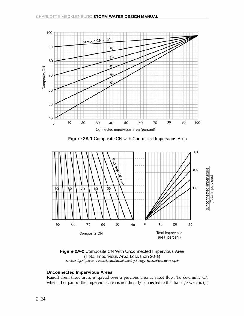
If all the impervious area is directly connected to the drainage system, but the impervious area percentages or the pervious land use assumptions in Table 2-12 are not applicable, use figure 2A-1 to compute composite CN. For example, Table 2-12 gives a CN of 70 for a ½ acre lot in hydrologic soil, group B, with an assumed impervious area of 25 percent. However, if the lot has 20 percent impervious area and a pervious area CN of 61, the composite CN obtained from Figure 2A-1 is 68. The CN difference between 70 and 68 reflects the difference in percent impervious area.
CHARLOTTE-MECKLENBURG STORM WATER DESIGN MANUAL
2-24
Figure 2A-1 Composite CN with Connected Impervious Area
Figure 2A-2 Composite CN With Unconnected Impervious Area (Total Impervious Area Less than 30%)
Source: ftp://ftp.wcc.nrcs.usda.gov/downloads/hydrology_hydraulicstr55/tr55.pdf
Unconnected Impervious Areas Runoff from these areas is spread over a pervious area as sheet flow. To determine CN when all or part of the impervious area is not directly connected to the drainage system, (1)
CHAPTER 2 HYDROLOGY
2-25
use Figure 2A-2 if total impervious area is less than 30 percent or (2) use Figure 2A-1 if the total impervious area is equal to or greater than 30 percent, because the absorptive capacity of the remaining pervious area will not significantly affect runoff.
When impervious area is less than 30 percent, obtain the composite CN by entering the right half of Figure 2A-2 with the percentage of total impervious area and the ratio of total unconnected impervious area to total impervious area. Then move left to the appropriate pervious CN and read down to find the composite CN. For example, for a ½ acre lot with 20 percent total impervious area (75 percent of which is unconnected) and pervious CN of 61, the composite CN from Figure 2A-2 is 66. If all of the impervious area is connected, the resulting CN (from Figure 2A-1) would be 68.
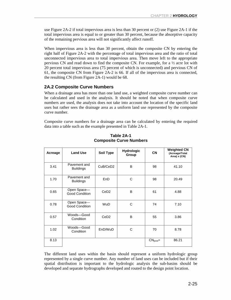
2A.2 Composite Curve Numbers When a drainage area has more than one land use, a weighted composite curve number can be calculated and used in the analysis. It should be noted that when composite curve numbers are used, the analysis does not take into account the location of the specific land uses but rather sees the drainage area as a uniform land use represented by the composite curve number.
Composite curve numbers for a drainage area can be calculated by entering the required data into a table such as the example presented in Table 2A-1.
Table 2A-1 Composite Curve Numbers
Acreage Land Use Soil Type Hydrologic
Group CN Weighted CN (Acreage/Total
Area) x (CN)
3.41 Pavement and Buildings CuB/CeD2 B 98 41.10
1.70 Pavement and Buildings EnD C 98 20.49
0.65 Open Space—Good Condition CeD2 B 61 4.88
0.78 Open Space—Good Condition WuD C 74 7.10
0.57 Woods—Good Condition CeD2 B 55 3.86
1.02 Woods—Good Condition EnD/WuD C 70 8.78
8.13 CNpost= 86.21
The different land uses within the basin should represent a uniform hydrologic group represented by a single curve number. Any number of land uses can be included but if their spatial distribution is important to the hydrologic analysis the sub-basins should be developed and separate hydrographs developed and routed to the design point location.
CHARLOTTE-MECKLENBURG STORM WATER DESIGN MANUAL
2-26
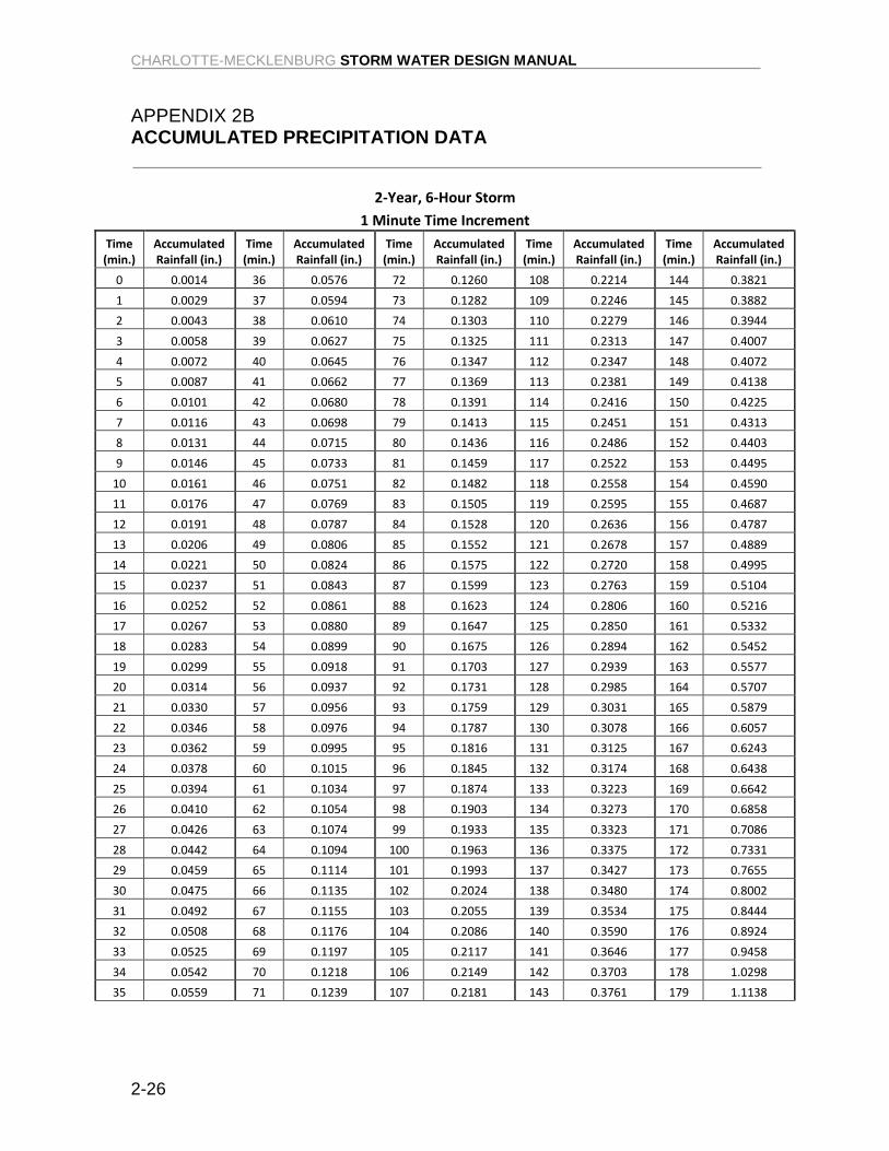
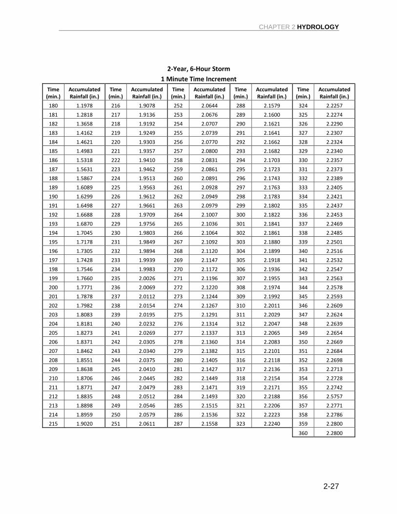
APPENDIX 2B ACCUMULATED PRECIPITATION DATA
2-Year, 6-Hour Storm 1 Minute Time Increment
Time (min.)
Accumulated Rainfall (in.)
Time (min.)
Accumulated Rainfall (in.)
Time (min.)
Accumulated Rainfall (in.)
Time (min.)
Accumulated Rainfall (in.)
Time (min.)
Accumulated Rainfall (in.)
0 0.0014 36 0.0576 72 0.1260 108 0.2214 144 0.3821 1 0.0029 37 0.0594 73 0.1282 109 0.2246 145 0.3882 2 0.0043 38 0.0610 74 0.1303 110 0.2279 146 0.3944 3 0.0058 39 0.0627 75 0.1325 111 0.2313 147 0.4007 4 0.0072 40 0.0645 76 0.1347 112 0.2347 148 0.4072 5 0.0087 41 0.0662 77 0.1369 113 0.2381 149 0.4138 6 0.0101 42 0.0680 78 0.1391 114 0.2416 150 0.4225 7 0.0116 43 0.0698 79 0.1413 115 0.2451 151 0.4313 8 0.0131 44 0.0715 80 0.1436 116 0.2486 152 0.4403 9 0.0146 45 0.0733 81 0.1459 117 0.2522 153 0.4495
10 0.0161 46 0.0751 82 0.1482 118 0.2558 154 0.4590 11 0.0176 47 0.0769 83 0.1505 119 0.2595 155 0.4687 12 0.0191 48 0.0787 84 0.1528 120 0.2636 156 0.4787 13 0.0206 49 0.0806 85 0.1552 121 0.2678 157 0.4889 14 0.0221 50 0.0824 86 0.1575 122 0.2720 158 0.4995 15 0.0237 51 0.0843 87 0.1599 123 0.2763 159 0.5104 16 0.0252 52 0.0861 88 0.1623 124 0.2806 160 0.5216 17 0.0267 53 0.0880 89 0.1647 125 0.2850 161 0.5332 18 0.0283 54 0.0899 90 0.1675 126 0.2894 162 0.5452 19 0.0299 55 0.0918 91 0.1703 127 0.2939 163 0.5577 20 0.0314 56 0.0937 92 0.1731 128 0.2985 164 0.5707 21 0.0330 57 0.0956 93 0.1759 129 0.3031 165 0.5879 22 0.0346 58 0.0976 94 0.1787 130 0.3078 166 0.6057 23 0.0362 59 0.0995 95 0.1816 131 0.3125 167 0.6243 24 0.0378 60 0.1015 96 0.1845 132 0.3174 168 0.6438 25 0.0394 61 0.1034 97 0.1874 133 0.3223 169 0.6642 26 0.0410 62 0.1054 98 0.1903 134 0.3273 170 0.6858 27 0.0426 63 0.1074 99 0.1933 135 0.3323 171 0.7086 28 0.0442 64 0.1094 100 0.1963 136 0.3375 172 0.7331 29 0.0459 65 0.1114 101 0.1993 137 0.3427 173 0.7655 30 0.0475 66 0.1135 102 0.2024 138 0.3480 174 0.8002 31 0.0492 67 0.1155 103 0.2055 139 0.3534 175 0.8444 32 0.0508 68 0.1176 104 0.2086 140 0.3590 176 0.8924 33 0.0525 69 0.1197 105 0.2117 141 0.3646 177 0.9458 34 0.0542 70 0.1218 106 0.2149 142 0.3703 178 1.0298 35 0.0559 71 0.1239 107 0.2181 143 0.3761 179 1.1138
CHAPTER 2 HYDROLOGY
2-27
2-Year, 6-Hour Storm 1 Minute Time Increment
Time (min.)
Accumulated Rainfall (in.)
Time (min.)
Accumulated Rainfall (in.)
Time (min.)
Accumulated Rainfall (in.)
Time (min.)
Accumulated Rainfall (in.)
Time (min.)
Accumulated Rainfall (in.)
180 1.1978 216 1.9078 252 2.0644 288 2.1579 324 2.2257 181 1.2818 217 1.9136 253 2.0676 289 2.1600 325 2.2274 182 1.3658 218 1.9192 254 2.0707 290 2.1621 326 2.2290 183 1.4162 219 1.9249 255 2.0739 291 2.1641 327 2.2307 184 1.4621 220 1.9303 256 2.0770 292 2.1662 328 2.2324 185 1.4983 221 1.9357 257 2.0800 293 2.1682 329 2.2340 186 1.5318 222 1.9410 258 2.0831 294 2.1703 330 2.2357 187 1.5631 223 1.9462 259 2.0861 295 2.1723 331 2.2373 188 1.5867 224 1.9513 260 2.0891 296 2.1743 332 2.2389 189 1.6089 225 1.9563 261 2.0928 297 2.1763 333 2.2405 190 1.6299 226 1.9612 262 2.0949 298 2.1783 334 2.2421 191 1.6498 227 1.9661 263 2.0979 299 2.1802 335 2.2437 192 1.6688 228 1.9709 264 2.1007 300 2.1822 336 2.2453 193 1.6870 229 1.9756 265 2.1036 301 2.1841 337 2.2469 194 1.7045 230 1.9803 266 2.1064 302 2.1861 338 2.2485 195 1.7178 231 1.9849 267 2.1092 303 2.1880 339 2.2501 196 1.7305 232 1.9894 268 2.1120 304 2.1899 340 2.2516 197 1.7428 233 1.9939 269 2.1147 305 2.1918 341 2.2532 198 1.7546 234 1.9983 270 2.1172 306 2.1936 342 2.2547 199 1.7660 235 2.0026 271 2.1196 307 2.1955 343 2.2563 200 1.7771 236 2.0069 272 2.1220 308 2.1974 344 2.2578 201 1.7878 237 2.0112 273 2.1244 309 2.1992 345 2.2593 202 1.7982 238 2.0154 274 2.1267 310 2.2011 346 2.2609 203 1.8083 239 2.0195 275 2.1291 311 2.2029 347 2.2624 204 1.8181 240 2.0232 276 2.1314 312 2.2047 348 2.2639 205 1.8273 241 2.0269 277 2.1337 313 2.2065 349 2.2654 206 1.8371 242 2.0305 278 2.1360 314 2.2083 350 2.2669 207 1.8462 243 2.0340 279 2.1382 315 2.2101 351 2.2684 208 1.8551 244 2.0375 280 2.1405 316 2.2118 352 2.2698 209 1.8638 245 2.0410 281 2.1427 317 2.2136 353 2.2713 210 1.8706 246 2.0445 282 2.1449 318 2.2154 354 2.2728 211 1.8771 247 2.0479 283 2.1471 319 2.2171 355 2.2742 212 1.8835 248 2.0512 284 2.1493 320 2.2188 356 2.5757 213 1.8898 249 2.0546 285 2.1515 321 2.2206 357 2.2771 214 1.8959 250 2.0579 286 2.1536 322 2.2223 358 2.2786 215 1.9020 251 2.0611 287 2.1558 323 2.2240 359 2.2800
360 2.2800
CHARLOTTE-MECKLENBURG STORM WATER DESIGN MANUAL
2-28
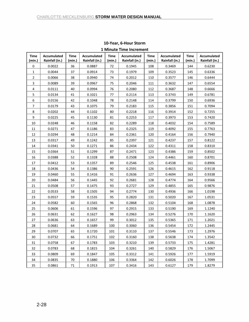
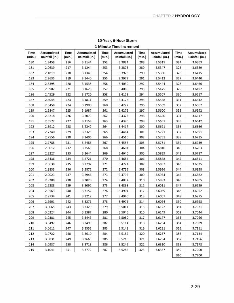
10-Year, 6-Hour Storm 1 Minute Time Increment
Time (min.)
Accumulated Rainfall (in.)
Time (min.)
Accumulated Rainfall (in.)
Time (min.)
Accumulated Rainfall (in.)
Time (min.)
Accumulated Rainfall (in.)
Time (min.)
Accumulated Rainfall (in.)
0 0.0022 36 0.0887 72 0.1945 108 0.3469 144 0.6230 1 0.0044 37 0.0914 73 0.1979 109 0.3523 145 0.6336 2 0.0066 38 0.0940 74 0.2012 110 0.3577 146 0.6444 3 0.0089 39 0.0967 75 0.2046 111 0.3632 147 0.6554 4 0.0111 40 0.0994 76 0.2080 112 0.3687 148 0.6666 5 0.0134 41 0.1021 77 0.2114 113 0.3743 149 0.6781 6 0.0156 42 0.1048 78 0.2148 114 0.3799 150 0.6936 7 0.0179 43 0.1075 79 0.2183 115 0.3856 151 0.7094 8 0.0202 44 0.1102 80 0.2218 116 0.3914 152 0.7255 9 0.0225 45 0.1130 81 0.2253 117 0.3973 153 0.7420
10 0.0248 46 0.1158 82 0.2289 118 0.4032 154 0.7589 11 0.0271 47 0.1186 83 0.2325 119 0.4092 155 0.7763 12 0.0294 48 0.1214 84 0.2361 120 0.4164 156 0.7940 13 0.0317 49 0.1242 85 0.2397 121 0.4237 157 0.8122 14 0.0341 50 0.1271 86 0.2434 122 0.4311 158 0.8310 15 0.0364 51 0.1299 87 0.2471 123 0.4386 159 0.8502 16 0.0388 52 0.1328 88 0.2508 124 0.4461 160 0.8701 17 0.0412 53 0.1357 89 0.2546 125 0.4538 161 0.8906 18 0.0436 54 0.1386 90 0.2591 126 0.4615 162 0.9118 19 0.0460 55 0.1416 91 0.2636 127 0.4694 163 0.9338 20 0.0484 56 0.1445 92 0.2681 128 0.4774 164 0.9566 21 0.0508 57 0.1475 93 0.2727 129 0.4855 165 0.9876 22 0.0533 58 0.1505 94 0.2774 130 0.4936 166 1.0198 23 0.0557 59 0.1535 95 0.2820 131 0.5020 167 1.0531 24 0.0582 60 0.1565 96 0.2868 132 0.5104 168 1.0878 25 0.0606 61 0.1596 97 0.2915 133 0.5190 169 1.1240 26 0.0631 62 0.1627 98 0.2963 134 0.5276 170 1.1620 27 0.0636 63 0.1657 99 0.3012 135 0.5365 171 1.2021 28 0.0681 64 0.1689 100 0.3060 136 0.5454 172 1.2445 29 0.0707 65 0.1720 101 0.3110 137 0.5546 173 1.2976 30 0.0732 66 0.1751 102 0.3160 138 0.5638 174 1.3542 31 0.0758 67 0.1783 103 0.3210 139 0.5733 175 1.4281 32 0.0783 68 0.1815 104 0.3261 140 0.5829 176 1.5067 33 0.0809 69 0.1847 105 0.3312 141 0.5926 177 1.5919 34 0.0835 70 0.1880 106 0.3364 142 0.6026 178 1.7099 35 0.0861 71 0.1913 107 0.3416 143 0.6127 179 1.8279
CHAPTER 2 HYDROLOGY
2-29
10-Year, 6-Hour Storm 1 Minute Time Increment
Time (min.)
Accumulated Rainfall (in.)
Time (min.)
Accumulated Rainfall (in.)
Time (min.)
Accumulated Rainfall (in.)
Time (min.)
Accumulated Rainfall (in.)
Time (min.)
Accumulated Rainfall (in.)
180 1.9459 216 3.1144 252 3.3824 288 3.5315 324 3.6363 181 2.0639 217 3.1244 253 3.3876 289 3.5347 325 3.6389 182 2.1819 218 3.1343 254 3.3928 290 3.5380 326 3.6415 183 2.2635 219 3.1440 255 3.3979 291 3.5412 327 3.6440 184 2.3395 220 3.1535 256 3.4030 292 3.5444 328 3.6466 185 2.3982 221 3.1628 257 3.4080 293 3.5475 329 3.6492 186 2.4529 222 3.1720 258 3.4129 294 3.5507 330 3.6517 187 2.5045 223 3.1811 259 3.4178 295 3.5538 331 3.6542 188 2.5458 224 3.1900 260 3.4227 296 3.5569 332 3.6567 189 2.5847 225 3.1987 261 3.4275 297 3.5600 333 3.6592 190 2.6218 226 3.2073 262 3.4323 298 3.5630 334 3.6617 191 2.6572 227 3.2158 263 3.4370 299 3.5661 335 3.6642 192 2.6912 228 3.2242 264 3.4417 300 3.5691 336 3.6666 193 2.7240 229 3.2325 265 3.4464 301 3.5721 337 3.6691 194 2.7556 230 3.2406 266 3.4510 302 3.5751 338 3.6715 195 2.7788 231 3.2486 267 3.4556 303 3.5781 339 3.6739 196 2.8012 232 3.2565 268 3.4601 304 3.5810 340 3.6763 197 2.8227 233 3.2644 269 3.4646 305 3.5839 341 3.6787 198 2.8436 234 3.2721 270 3.4684 306 3.5868 342 3.6811 199 2.8638 235 3.2797 271 3.4721 307 3.5897 343 3.6835 200 2.8833 236 3.2872 272 3.4759 308 3.5926 344 3.6858 201 2.9023 237 3.2946 273 3.4795 309 3.5954 345 3.6882 202 2.9208 238 3.3020 274 3.4832 310 3.5983 346 3.6905 203 2.9388 239 3.3092 275 3.4868 311 3.6011 347 3.6929 204 2.9563 240 3.3152 276 3.4904 312 3.6039 348 3.6952 205 2.9734 241 3.3212 277 3.4940 313 3.6067 349 3.6975 206 2.9901 242 3.3271 278 3.4975 314 3.6094 350 3.6998 207 3.0065 243 3.3329 279 3.5011 315 3.6122 351 3.7021 208 3.0224 244 3.3387 280 3.5045 316 3.6149 352 3.7044 209 3.0381 245 3.3443 281 3.5080 317 3.6177 353 3.7066 210 3.0497 246 3.3499 282 3.5114 318 3.6204 354 3.7089 211 3.0611 247 3.3555 283 3.5148 319 3.6231 355 3.7111 212 3.0722 248 3.3610 284 3.5182 320 3.6257 356 3.7134 213 3.0831 249 3.3665 285 3.5216 321 3.6284 357 3.7156 214 3.0937 250 3.3718 286 3.5249 322 3.6310 358 3.7178 215 3.1041 251 3.3772 287 3.5282 323 3.6337 359 3.7200
360 3.7200
CHARLOTTE-MECKLENBURG STORM WATER DESIGN MANUAL
2-30
50-Year, 6-Hour Storm 1 Minute Time Increment
Time (min.)
Accumulated Rainfall (in.)
Time (min.)
Accumulated Rainfall (in.)
Time (min.)
Accumulated Rainfall (in.)
Time (min.)
Accumulated Rainfall (in.)
Time (min.)
Accumulated Rainfall (in.)
0 0.0031 36 0.1257 72 0.2750 108 0.4847 144 0.8583 1 0.0063 37 0.1295 73 0.2797 109 0.4919 145 0.8725 2 0.0094 38 0.1332 74 0.2844 110 0.4992 146 0.8870 3 0.0126 39 0.1370 75 0.2891 111 0.5066 147 0.9018 4 0.0158 40 0.1408 76 0.2939 112 0.5141 148 0.9170 5 0.0189 41 0.1446 77 0.2987 113 0.5217 149 0.9324 6 0.0221 42 0.1484 78 0.3036 114 0.5293 150 0.9526 7 0.0254 43 0.1523 79 0.3084 115 0.5370 151 0.9733 8 0.0286 44 0.1562 80 0.3134 116 0.5449 152 0.9944 9 0.0319 45 0.1601 81 0.3183 117 0.5528 153 1.0159
10 0.0351 46 0.1640 82 0.3233 118 0.5608 154 1.0380 11 0.0384 47 0.1679 83 0.3283 119 0.5689 155 1.0606 12 0.0417 48 0.1719 84 0.3334 120 0.5787 156 1.0838 13 0.0450 49 0.1759 85 0.3385 121 0.5886 157 1.1076 14 0.0483 50 0.1799 86 0.3437 122 0.5986 158 1.1320 15 0.0517 51 0.1839 87 0.3489 123 0.6087 159 1.1571 16 0.0550 52 0.1880 88 0.3542 124 0.6190 160 1.1830 17 0.0584 53 0.1921 89 0.3594 125 0.6294 161 1.2098 18 0.0618 54 0.1962 90 0.3655 126 0.6399 162 1.2374 19 0.0652 55 0.2004 91 0.3717 127 0.6506 163 1.2660 20 0.0686 56 0.2045 92 0.3778 128 0.6614 164 1.2957 21 0.0720 57 0.2087 93 0.3841 129 0.6723 165 1.3363 22 0.0755 58 0.2129 94 0.3903 130 0.6834 166 1.3783 23 0.0790 59 0.2172 95 0.3967 131 0.6947 167 1.4219 24 0.0825 60 0.2215 96 0.4031 132 0.7061 168 1.4672 25 0.0860 61 0.2258 97 0.4095 133 0.7177 169 1.5145 26 0.0895 62 0.2301 98 0.4160 134 0.7294 170 1.5640 27 0.0930 63 0.2344 99 0.4226 135 0.7414 171 1.6161 28 0.0966 64 0.2388 100 0.4292 136 0.7535 172 1.6714 29 0.1002 65 0.2432 101 0.4359 137 0.7658 173 1.7400 30 0.1038 66 0.2477 102 0.4427 138 0.7783 174 1.8130 31 0.1074 67 0.2522 103 0.4495 139 0.7911 175 1.9086 32 0.1110 68 0.2567 104 0.4564 140 0.8040 176 2.0101 33 0.1147 69 0.2612 105 0.4634 141 0.8172 177 2.1198 34 0.1183 70 0.2658 106 0.4704 142 0.8307 178 2.2698 35 0.1220 71 0.2704 107 0.4775 143 0.8443 179 2.4198
CHAPTER 2 HYDROLOGY
2-31
50-Year, 6-Hour Storm 1 Minute Time Increment
Time (min.)
Accumulated Rainfall (in.)
Time (min.)
Accumulated Rainfall (in.)
Time (min.)
Accumulated Rainfall (in.)
Time (min.)
Accumulated Rainfall (in.)
Time (min.)
Accumulated Rainfall (in.)
180 2.5698 216 4.0852 252 4.4480 288 4.6535 324 4.8014 181 2.7198 217 4.0988 253 4.4551 289 4.6581 325 4.8051 182 2.8698 218 4.1121 254 4.4621 290 4.6626 326 4.8087 183 2.9751 219 4.1252 255 4.4690 291 4.6671 327 4.8124 184 3.0734 220 4.1380 256 4.4758 292 4.6716 328 4.8160 185 3.1490 221 4.1507 257 4.4826 293 4.6761 329 4.8196 186 3.2197 222 4.1631 258 4.4893 294 4.6805 330 4.8232 187 3.2864 223 4.1753 259 4.4960 295 4.6849 331 4.8268 188 3.3401 224 4.1873 260 4.5026 296 4.6893 332 4.8303 189 3.3908 225 4.1992 261 4.5092 297 4.6936 333 4.8338 190 3.4392 226 4.2109 262 4.5156 298 4.6980 334 4.8374 191 3.4854 227 4.2224 263 4.5221 299 4.7022 335 4.8409 192 3.5298 228 4.2337 264 4.5284 300 4.7065 336 4.8443 193 3.5726 229 4.2449 265 4.5347 301 4.7107 337 4.8478 194 3.6139 230 4.2559 266 4.5410 302 4.7149 338 4.8512 195 3.6442 231 4.2668 267 4.5472 303 4.7191 339 4.8547 196 3.6733 232 4.2775 268 4.5533 304 4.7233 340 4.8581 197 3.7014 233 4.2881 269 4.5594 305 4.7274 341 4.8615 198 3.7286 234 4.2985 270 4.5648 306 4.7315 342 4.8649 199 3.7549 235 4.3089 271 4.5700 307 4.7356 343 4.8682 200 3.7804 236 4.3191 272 4.5753 308 4.7396 344 4.8716 201 3.8052 237 4.3291 273 4.5804 309 4.7437 345 4.8749 202 3.8293 238 4.3391 274 4.5856 310 4.7477 346 4.8782 203 3.8528 239 4.3489 275 4.5907 311 4.7516 347 4.8815 204 3.8757 240 4.3571 276 4.5957 312 4.7556 348 4.8848 205 3.8980 241 4.3651 277 4.6008 313 4.7595 349 4.8881 206 3.9198 242 4.3731 278 4.6057 314 4.7635 350 4.8913 207 3.9411 243 4.3810 279 4.6107 315 4.7673 351 4.8946 208 3.9620 244 4.3888 280 4.6156 316 4.7712 352 4.8978 209 3.9824 245 4.3965 281 4.6204 317 4.7751 353 4.9010 210 3.9981 246 4.4041 282 4.6253 318 4.7789 354 4.9042 211 4.0134 247 4.4116 283 4.6301 319 4.7827 355 4.9074 212 4.0283 248 4.4190 284 4.6348 320 4.7865 356 4.9106 213 4.0430 249 4.4264 285 4.6395 321 4.7902 357 4.9137 214 4.0574 250 4.4337 286 4.6442 322 4.7940 358 4.9169 215 4.0714 251 4.4409 287 4.6489 323 4.7977 359 4.9200
360 4.9200