Chapter 2 Existence Theory and Properties of Solutions

Chapter 2

Existence Theory and Properties ofSolutions

This chapter contains some of the most important results of the course. Our first goal is toprove a theorem that guarantees the existence and uniqueness of a solution to an initial valueproblem on some, possibly small, interval. We then investigate the issue of how large thisinterval might be. The last section of the chapter provides some insight into how a solutionof an initial value problem changes when the differential equation or initial conditions arealtered.

2.1 Introduction

Consider an nth order differential equation in the form

y(n) = g(t, y, y′, y′′, · · · , y(n−1)).

It is a standard practice to convert such an nth order equation into a first order system bydefining

x1 = yx2 = y′

...xn = y(n−1).

We will denote vectors in Rn by x = (x1, · · ·xn) so that our scalar equation is now representedin vector form as

dx

dt= x′(t) =

x2

x3...g(t, x1, x2, · · · , xn)

= f(t, x(t)).

1

2 CHAPTER 2. EXISTENCE THEORY AND PROPERTIES OF SOLUTIONS

Consequently it suffices to focus upon 1st ordinary differential equations denoted by

x′(t) = f(t, x(t)) (2.1.1)

where x ∈ Rn and f(t, x) ∈ Rn is defined on an open set U ⊆ R×Rn. A solution of (2.1.1)is a differentiable function

ξ : J → Rn

where J is an open interval in R and for t ∈ J , (t, ξ(t)) ∈ U , and

ξ′(t) = f(t, ξ(t)).

A solution ξ(t) of the initial value problem (IVP)

x′(t) = f(t, x(t))

x(t0) = x0.(2.1.2)

is a solution of the differential equation (2.1.1) that also satisfies the initial condition ξ(t0) =x0.

Example 2.1.1 Rcall from Example (1.2.3) that the IVP

x′ =x

t+ t = f(t, x)

x(0) = x0

has infinitely many solutions if x0 = 0 and no solution if x0 6= 0. This suggests that continuityof f(t, x) would be a minimal condition to ensure existence of a solution to an IVP.

Example 2.1.2 Consider

x′ = f(t, x) = x1/3.

By separation of variables we get the family of solutions

ξ(t) = (2

3(t+ c))3/2

Now consider the IVP

x′ = x1/3

x(0) = 0.

2.1. INTRODUCTION 3

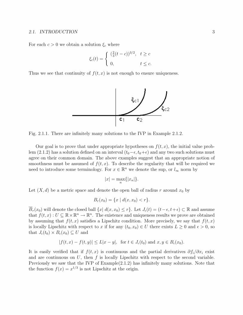
For each c > 0 we obtain a solution ξc where

ξc(t) =

{(2

3(t− c))3/2, t ≥ c

0, t ≤ c.

Thus we see that continuity of f(t, x) is not enough to ensure uniqueness.

Fig. 2.1.1. There are infinitely many solutions to the IVP in Example 2.1.2.

Our goal is to prove that under appropriate hypotheses on f(t, x), the initial value prob-lem (2.1.2) has a solution defined on an interval (t0−ε, t0+ε) and any two such solutions mustagree on their common domain. The above examples suggest that an appropriate notion ofsmoothness must be assumed of f(t, x). To describe the regularity that will be required weneed to introduce some terminology. For x ∈ Rn we denote the sup, or l∞ norm by

|x| = maxn{|xn|}.

Let (X, d) be a metric space and denote the open ball of radius r around x0 by

Br(x0) = {x | d(x, x0) < r}.

Br(x0) will denote the closed ball {x| d(x, x0) ≤ r}. Let Jε(t) = (t−ε, t+ε) ⊂ R and assumethat f(t, x) : U ⊆ R×Rn → Rn. The existence and uniqueness results we prove are obtainedby assuming that f(t, x) satisfies a Lipschitz condition. More precisely, we say that f(t, x)is locally Lipschitz with respect to x if for any (t0, x0) ∈ U there exists L ≥ 0 and ε > 0, sothat Jε(t0)×Bε(x0) ⊆ U and

|f(t, x)− f(t, y)| ≤ L|x− y|, for t ∈ Jε(t0) and x, y ∈ Bε(x0).

It is easily verified that if f(t, x) is continuous and the partial derivatives ∂fi/∂xi existand are continuous on U , then f is locally Lipschitz with respect to the second variable.Previously we saw that the IVP of Example(2.1.2) has infinitely many solutions. Note thatthe function f(x) = x1/3 is not Lipschitz at the origin.


The notion of a contractive mapping is central to many existence arguments. If α statisfies0 < α < 1, and T : X → X is a mapping, we say T is an α-contraction if

d(T (x), T (y)) ≤ αd(x, y) for all x, y ∈ X.

If T (p) = p, we call p is a fixed point of T . We will denote iterates of T by

T 0(x) = x, T 1(x) = T (x), T 2(x) = T (T 1(x)), · · · T n(x) = T (T n−1(x)).

The following lemma is crucial.

Lemma 2.1.1 [Contraction Mapping Lemma]. Let (X, d) be a complete metric spaceand T : X → X an α-contraction. Then T has a unique fixed point p. In fact, for anyx ∈ X, the iterates T n(x) converge to p.

Proof. Define f : X → [0,∞) by f(x) = d(T (x), x). In other words, f(x) is the distanceT moves x. Note that f(p) = 0 if T (p) = p and observe that f is continuous. Indeed

f(x) = d(x, T (x))

≤ d(x, y) + d(y, T (y)) + (T (y), T (x))

≤ d(x, y) + f(y) + αd(x, y)

and sof(x)− f(y) ≤ (1 + α)d(x, y).

Interchanging x and y we see

|f(x)− f(y)| ≤ (1 + α)d(x, y).

There are two inequalities satisfied by f . First,

f(T (x)) = d(T (T (x)), T (x)) ≤ αd(T (x), x) = αf(x). (2.1.3)

For the second inequality note that for x, y ∈ X,

d(x, y) ≤ d(x, T (x)) + d(T (x), T (y)) + d(T (y), y)

≤ f(x) + αd(x, y) + f(y)

and so

d(x, y) ≤ f(x) + f(y)

1− α . (2.1.4)

2.2. EXISTENCE AND UNIQUENESS OF SOLUTIONS 5

Now let x0 be any point in X and xn = T n(x0). Then from (2.1.3)

f(xn) ≤ αnf(x0)

and so f(xn)→ 0 as n→∞. It follows from (2.1.4) that for any n,m

d(xn, xm) ≤ f(xn) + f(xm)

1− α .

For n,m sufficiently large we can make the right hand side as small as we like and hence{xn} is a Cauchy sequence. Since X is complete, there exists a p ∈ X such that xn → p.Because f is continuous, f(xn)→ f(p), and so f(p) = 0, i.e., p is a fixed point of T .

To show uniqueness suppose q is another fixed point. Then f(q) = 0 and from (2.1.4) wesee d(p, q) = 0.

2.2 Existence and Uniqueness of Solutions

It turns out that continuity of f(t, x) is sufficient to guarantee existence of a solution to theIVP

x′(t) = f(t, x(t))

x(t0) = x0.

This result is referred to as Peano’s Theorem. Example (2.1.2) in the previous section showedthat we need additional hypotheses on f(t, x) to ensure uniqueness. The condition we needis Lipschitz continuity.

The next theorem is a first form of our Existence and Uniqueness Theorem.

Theorem 2.2.1 Let f : U ⊆ R× Rn → Rn, U open and f(t, x) continuous and locallyLipschitz with respect to the second variable. The following two statements hold.

(1) Select (t0, x0) ∈ U . For all ε > 0 sufficiently small there is a differentiable functionξ : (t0 − ε, t0 + ε)→ Rn such that

(t, ξ(t)) ∈ U, t ∈ Jε(t0)

ξ′(t) = f(t, ξ(t)), t ∈ Jε(t0)

ξ(t0) = x0.

(2.2.1)

That is, ξ is a solution of the initial value problem.

(2) If ξ1 : Jε1(t0) → Rn and ξ2 : Jε2(t0) → Rn are two differentiable functions that satisfy(2.2.1), then ξ1 and ξ2 agree on some open interval around t0.


First we need the following lemma.

Lemma 2.2.1 A function ξ : Jε(t0) → Rn is differentiable and satisfies (2.2.1) if andonly if for t ∈ Jε(t0), (t, ξ(t)) ∈ U , ξ is continuous, and satisfies

ξ(t) = x0 +

∫ t

t0

f(s, ξ(s))ds, t ∈ Jε(t0). (2.2.2)

Proof. Let ξ be a differentiable function that satisfies (2.2.1). Since ξ′(t) = f(t, ξ(t))and f is continuous, ξ′ is continuous. Thus by the Fundamental Theorem of Calculus∫ t

t0

ξ′(s)ds = ξ(t)− ξ(t0) = ξ(t)− x0 =

∫ t

t0

f(s, ξ(s)) ds

and so ξ(t) satisfies (2.2.2).Conversely suppose ξ satisfies the conditions of the second part of the lemma. Then

clearlyξ(t0) = x0

and by the Fundamental Theorem of Calculus,

ξ′(t) = f(t, ξ(t)).

Thus ξ is differentiable and satisfies the IVP.

The proof of Theorem(2.2.1) is based on the Contractive Mapping Lemma where theunderlying metric space will be a closed subset of BC(Jε(t0);Rn), the space of boundedcontinuous functions

ξ : Jε(t0)→ Rn

where for ξ1, ξ2 ∈ BC(Jε(t0)),

d(ξ1, ξ2) = supt∈Jε(t0)

{|(ξ1 − ξ2)(t)|}

= ||ξ1 − ξ2||.

Proof of Theorem 2.2.1. Since f is locally Lipschitz with respect to the secondvariable, we can find an r > 0 such that [t0 − r, t0 + r]×Br(x0) ⊂ U and

|f(t, x)− f(t, y| ≤ L|x− y| for all (t, x), (t, y) ∈ [t0 − r, t0 + r]×Br(x0).


Since [t0 − r, t0 + r]×Br(x0) is compact and f is continuous, there exists an M for which

|f(t, x)| ≤M for all (t, x) ∈ [t0 − r, t0 + r]×Br(x0).

Choose ε > 0 so small such that

ε < r

εM < r

εL < 1.

Let X ⊂ BC(Jε(t0);Rn) be the space of continuous functions

ξ : Jε(t0)→ Br(x0).

Then X is a closed subset of BC(Jε(t0);Rn) and hence is complete. Note that if ξ ∈ X, t ∈Jε(t0) and ε < r, then we certainly have (t, ξ(t)) ∈ Jε(t0) × Br(x0) ⊆ U. For ξ ∈ X, defineTξ on Jε(t0) by

Tξ(t) = x0 +

∫ t

t0

f(s, ξ(s))ds.

By the Fundamental Theorem of Calculus Tξ is continuous and

|Tξ(t)− x0| = |∫ t

t0

f(s, ξ(s))ds| ≤ |∫ t

t0

|f(s, ξ(s)|ds|

≤M |t− t0| < εM < r.

Hence Tξ(t) ∈ Br(x0) and so Tξ ∈ X. Thus T : X → X.We now show T is a contraction. If ξ, ζ ∈ X,

| Tξ(t)− Tζ(t)| = | x0 +

∫ t

t0

f(s, ξ(s)) ds− x0 −∫ t

t0

f(s, ζ(s)) ds |

≤∫ t

t0

| f(s, ξ(s))− f(s, ζ(s)) | ds |

≤ L|∫ t

t0

| ξ(s)− ζ(s) | ds |

≤ L|∫ t

t0

||ξ − ζ|| ds |

= L|t− t0| ||ξ − ζ||

≤ εL||ξ − ζ||.


Thus

supt∈Jε(t0)

|Tξ(t)− Tζ(t)| = ||Tξ − Tζ|| ≤ ε L||ξ − ζ||

and since εL < 1, T is a contraction. Hence T has a fixed point and so there exists ξ ∈ Xsuch that

Tξ(t) = ξ(t) = x0 +

∫ t

t0

f(s, ξ(s))ds.

By Lemma(2.2.1), this ξ(t) is a solution (2.2.1)

Before proceeding to the proof of the second statement, note that given (t0, x0) we firstchoose r such that Kr = [t0 − r, t0 + r]×Br(x0) ⊂ U. Once we select ε so that ε < r, εM <r, εL < 1, we can consider the set X ⊆ BC(Jε(t0);Rn) in which T has a fixed point. Inthis sense the set X may be regarded as a one-paremeter family X(ε) and the fixed point,though unique in X(ε), does depend on ε.

To prove the second statement of the proposition suppose ξ1, ξ2 are two solutions of theIVP. The intersection of their domains is an open interval, say (t0− ε, t0 + ε). Since ξ1(t0) =ξ2(t0) = x0, and ξ1, ξ2 are continuous we can select ε such that ξ1, ξ2 : Jε(t0) → Br(x0). Wecan further decrease ε if necessary so that ε < r, εM < r and εL < 1. With this choiceof ε, we then get that ξ1, ξ2 ∈ X(ε) and since T : X(ε) → X(ε) has a unique fixed point,ξ1(t) = ξ2(t), t ∈ Jε(t0).

In summary, we have that for (t0, x0) ∈ U there exists ε > 0 such that the IVP has asolution ξ that is defined on (t0 − ε, t0 + ε) if ε < r, εM < r, εL < 1. Note that in showingTξ(t) ∈ Br(x0) we showed all iterates satisfy

|Tξ − x0| ≤M |t− t0| < Mε.

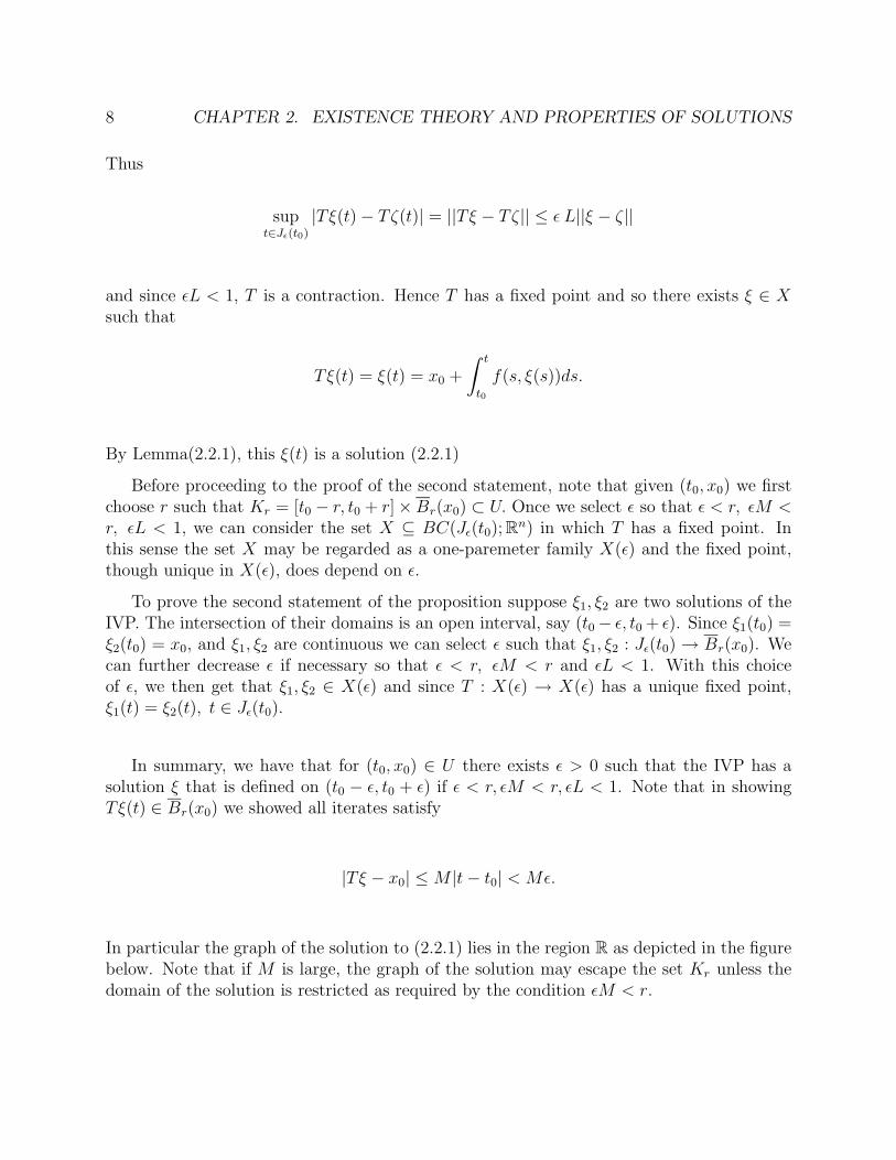
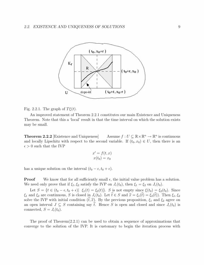
In particular the graph of the solution to (2.2.1) lies in the region R as depicted in the figurebelow. Note that if M is large, the graph of the solution may escape the set Kr unless thedomain of the solution is restricted as required by the condition εM < r.


Fig. 2.2.1. The graph of Tξ(t).

An improved statement of Theorem 2.2.1 constitutes our main Existence and UniquenessTheorem. Note that this a ‘local’ result in that the time interval on which the solution existsmay be small.

Theorem 2.2.2 [Existence and Uniqueness] Assume f : U ⊆ R×Rn → Rn is continuousand locally Lipschitz with respect to the second variable. If (t0, x0) ∈ U , then there is anε > 0 such that the IVP

x′ = f(t, x)x(t0) = x0

has a unique solution on the interval (t0 − ε, t0 + ε).

Proof We know that for all sufficiently small ε, the initial value problem has a solution.We need only prove that if ξ1, ξ2 satisfy the IVP on Jε(t0), then ξ1 = ξ2 on Jε(t0).

Let S = {t ∈ (t0 − ε, t0 + ε)| ξ1(t) = ξ2(t)}. S is not empty since ξ(t0) = ξ2(t0). Sinceξ1 and ξ2 are continuous, S is closed in Jε(t0). Let t̂ ∈ S and x̂ = ξ1(t̂) = ξ2(t̂)). Then ξ1, ξ2

solve the IVP with initial condition (t̂, x̂). By the previous proposition, ξ1 and ξ2 agree onan open interval J ⊆ S containing say t̂. Hence S is open and closed and since Jε(t0) isconnected, S = Jε(t0).

The proof of Theorem(2.2.1) can be used to obtain a sequence of approximations thatconverge to the solution of the IVP. It is customary to begin the iteration process with


x(t) = x0. Then

x1(t) = Tx = x0 +

∫ t

t0

f(s, x0)ds

x2(t) = T 2x = x0 +

∫ t

t0

f(s, x1(s))ds

......

xn(t) = T nx = x0 +

∫ t

t0

f(s, xn−1(s))ds.

From our results we know that {xn(t)} converges to a solution of the IVP in some neigh-borhood of t0. This sequence of approximate solutions are known as Picard iterates. Theusefulness of approximating a solution by this procedure has been somewhat enhanced bythe availability of computer algebra systems such and Maple and Mathematica.

2.3 Continuation and Maximal Intervals of Existence

Our existence theorem is of local nature in that it provides for the existence of a solution tothe IVP

x′(t) = f(t, x(t))

x(t0) = x0

defined in an interval (t0 − ε, t0 + ε)

Example 2.3.1 The solution of

x′ = x2

x(0) = 1

is

x(t) =1

1− tHere U = R×R. Note that the solution is defined for −∞ < t < 1. As t→ 1−, the graph ofthe x(t) leaves every closed and bounded subset of U . We will prove a theorem that reflectsthis general behavior. That is, the solution of an IVP can be defined on an interval (m1,m2)where either m2 = +∞ or the graph of the solution escapes every closed and bounded subsetof U as x→ m2 (and similarly for m1).

2.3. CONTINUATION AND MAXIMAL INTERVALS OF EXISTENCE 11

Throughout this section we suppose f : U ⊆ R × Rn → Rn, U open, and f(t, x) iscontinuous on U and locally Lipschitz in x. Suppose ξ(t) is a solution of

x′ = f(t, x)x(t0) = x0

that is defined for γ < t < δ and (δ, ξ(δ−)) ∈ U . Now consider the IVP

x′ = f(t, x)x(δ) = ξ(δ−).

We know this problem has a solution, say ψ(t), defined on δ ≤ t < δ + ε. Define

y(t) =

{ξ(t) γ < t < δψ(t) δ ≤ t < δ + ε.

Clearly y(t) is continuous. Moreover,

y(t) = ξ(δ−) +

∫ t

δ

f(s, ψ(s)) ds for δ ≤ t < δ + ε

and

ξ(δ−) = x0 +

∫ δ

x0

f(s, ξ(s))ds.

Hence

y(t) = x0 +

∫ δ

t0

f(s, ξ(s)ds+

∫ t

δ

f(s, ψ(s))ds

or

y(t) = x0 +

∫ t

t0

f(s, y(s))ds, δ ≤ t < δ + ε.

Since we clearly have

y(t) = x0 +

∫ t

t0

f(s, y(s))ds, γ < t < δ,

it follows from Lemma(2.2.1) that

y′(t) = f(t, y(t)), γ < t < δ + ε

y(t0) = x0

and so y(t) is a solution of the IVP that is defined on a larger interval.

The above process is referred to as continuation to the right. In the same way one couldconstruct a continuation to the left. By our uniqueness result any extension of the solution


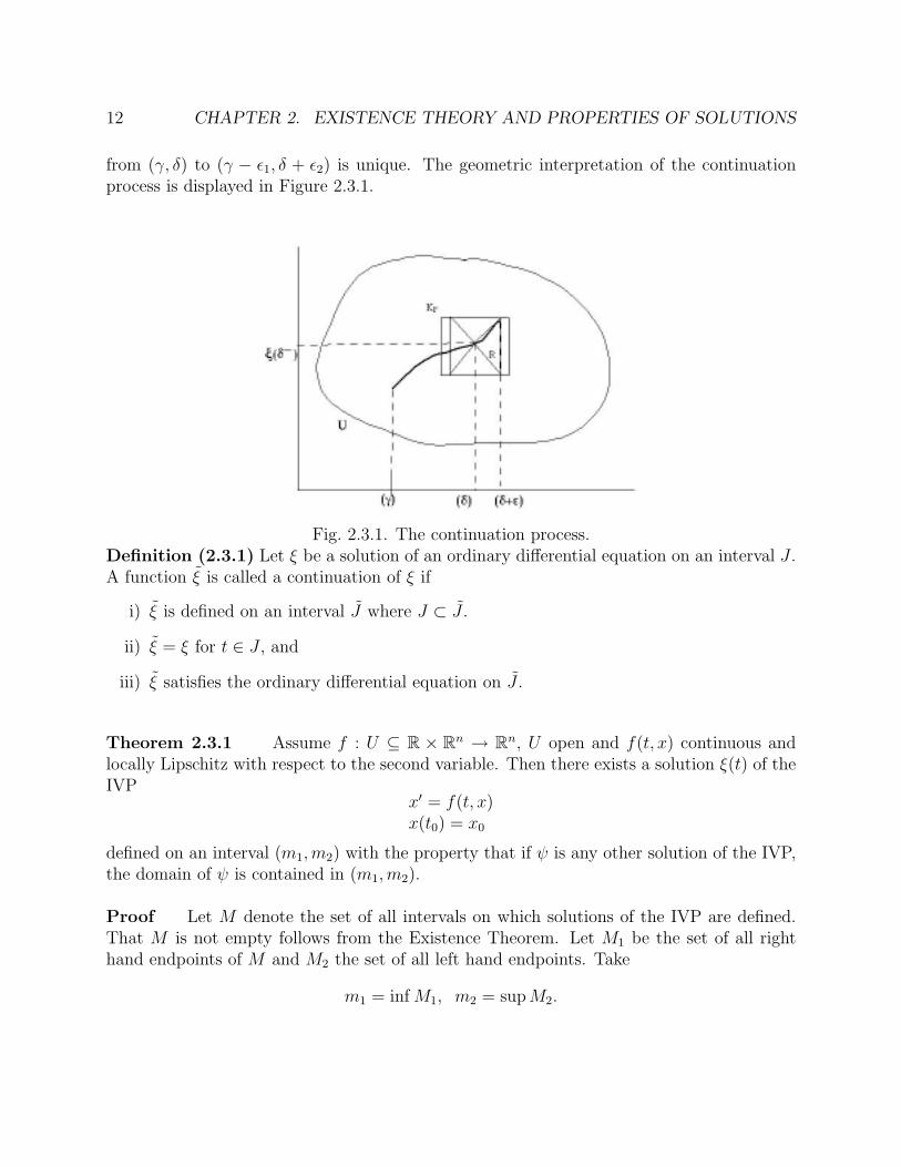
from (γ, δ) to (γ − ε1, δ + ε2) is unique. The geometric interpretation of the continuationprocess is displayed in Figure 2.3.1.

Fig. 2.3.1. The continuation process.Definition (2.3.1) Let ξ be a solution of an ordinary differential equation on an interval J .A function ξ̃ is called a continuation of ξ if

i) ξ̃ is defined on an interval J̃ where J ⊂ J̃ .

ii) ξ̃ = ξ for t ∈ J , and

iii) ξ̃ satisfies the ordinary differential equation on J̃ .

Theorem 2.3.1 Assume f : U ⊆ R × Rn → Rn, U open and f(t, x) continuous andlocally Lipschitz with respect to the second variable. Then there exists a solution ξ(t) of theIVP

x′ = f(t, x)x(t0) = x0

defined on an interval (m1,m2) with the property that if ψ is any other solution of the IVP,the domain of ψ is contained in (m1,m2).

Proof Let M denote the set of all intervals on which solutions of the IVP are defined.That M is not empty follows from the Existence Theorem. Let M1 be the set of all righthand endpoints of M and M2 the set of all left hand endpoints. Take

m1 = inf M1, m2 = supM2.


Pick any t̂ ∈ (m1,m2). Then there exists a solution of the IVP whose interval of definition

includes t̂, say ξ̂. Define a solution ξ(t) on (m1,m2) by setting ξ(t̂) = ξ̂(t̂). By uniqueness itfollows that ξ(t) is well defined and is a solution for all t ∈ (m1,m2).

The interval (m1,m2) is called the maximal interval of existence corresponding to (t0, x0).Furthermore, the maximal interval must be open (verify this).

Example 2.3.2 Take U to be the right half plane and consider

x′(t) =1

t2cos(

1

t)

x(t0) = x0

Then x(t) = c − sin(1t) and the IVP can be solved for any inital condition (t0, x0), t0 > 0.

Note that the maximal interval of existence is (0,∞) and limt→0+ x(t) does not exist.

Example 2.3.3 Considerx′ = −3x4/3 sin(t)

x(t0) = x0.

Solutions are x(t) ≡ 0 and x(t) = (c − cos t)−3 where c is determined by the initial data(t0, x0). Nontrivial solutions are defined on (−∞,∞) only if |c| > 1. Thus, the the maximalinterval of existence may depend on the initial conditions. Moreover, this example andExample(2.3.1) suggest that the graph of a solution tends to infinity at a finite endpoint ofthe maximal interval of existence. This is indeed the case when f(t, x) is bounded, but thecomplete story is a bit more involved. The next few theorems address this issue and clarifythese suggestions.

Theorem 2.3.2 Assume f : U ⊆ R × Rn → Rn, U open and f(t, x) continuous andlocally Lipschitz with respect to the second variable and bounded on U . If ξ(t) is a solutionof the IVP,

x′(t) = f(t, x)

x(t0) = x0

and defined for γ < t < δ, then the limits

limt→γ+

ξ(t), limt→δ−

ξ(t)

exist. If (δ, ξ(δ−)), (γ, ξ(γ+)) ∈ U , then the solution can be extended to the right and left.


Proof Let t1, t2 ∈ (γ, δ). Then

|ξ(t1)− ξ(t2)| ≤ |∫ t1

t2

|f(s, ξ(s))|ds|

≤ B|t1 − t2|.

If we pick {tn} such that tn → δ−, then for any ε > 0,

|ξ(tn)− ξ(tm)| ≤ B|tn − tm| < ε

for all n,m sufficiently large. Hence {ξ(tn)} is Cauchy and so converges. Thus limn→∞ ξ(tn)exists. An identical argument applies for limt→δ− ξ(t).

The second assertion follows immediately from the remarks preceding the definition ofcontinuation.

Compare this theorem with the result of Example(2.3.2) in which f(t, x) = 1t2

cos(1t)

was not bounded on U . As we observed, the solution did not have a limit at the left handendpoint of its maximal interval of existence.

Theorem 2.3.3 Assume f : U ⊆ R × Rn → Rn, U open and f(t, x) continuous andlocally Lipschitz with respect to the second variable and bounded on U . Let (m1,m2) denotethe maximal interval of existence of the solution ξ of the IVP

x′ = f(t, x)

x(t0) = x0.

Then either m2 =∞ or (m2, ξ(m−2 )) is on the boundary of U . A similar statement holds for

m1.

Proof. First suppose m2 < ∞ were finite. From the previous theorem, ξ(m−2 ) existsand if (m2, ξ(m

−2 )) ∈ U then the solution could be extended to the right. It must follow that

(m2, ξ(m−2 )) lies on the boundary of U . Similarly for m1.

Example 2.3.4 Reconsider the example

x′ = x2

x(0) = 1

Here U = R2 and ξ(t) = 11−t . Define

UA = {(t, x) | |t| <∞, |x| < A}.


The maximal interval of existence is (m1,m2) = (−∞, 1) and as t → m−2 the graph of thesolution will always meet the boundary of UA when t = 1− 1/A.

In general suppose f(t, x) is is continuous and locally Lipschitz with respect to the secondvariable on all of R × Rn and the solution of an IVP has a maximal interval of existence,(m1,m2) where m2 < ∞. One may modify the ideas in the previous example and applyTheorem(2.3.2) to conclude that as t → m−2 the graph of the solution always meets theboundary |x| = A of the set UA. Since A can be arbitrarily large, the following theoremmust follow. (The details are left as an exercise.)

Corollary 2.3.1 Let U = R×Rn and (m1,m2) denote the maximal interval of existenceof the IVP. If |m2| <∞, then

limt→m−2

|ξ(t)| =∞.

(Similarly for m1).

This corollary provides a method for determining when a solution is global, that is,defined for all time t. In particular, if f(t, x) is defined on all of R× Rn, then a solution isglobal if it does not blow up in finite time. These ideas are illustrated in the next examples.

Example 2.3.5 Consider the equation for the damped, nonlinear pendulum.

y′′(t) + αy′ + sin y = 0, α > 0

y(0) = y0, y′(0) = v0.

Rewrite the problem as a first order system,

x1 = y

x2 = y′.

Then

x′ =d

dt

(x1

x2

)=

(x2

−αx2 − sin x1

)= f(x)

x(0) =

(y0

v0

).

Since ∂fi/∂xj are continuous for all (x1, x2), f is locally Lipschitz. Hence for any intitialconditions the IVP has a unique solution. We now show the solution is global, i.e., it existsfor all t.


In a standard way, one first multiplies the equation by y′ to get

y′(y′′ + αy′ + sin y) = 0

andd

dt(1

2(y′)2 − cos y) = −α(y′)2 ≤ 0

ord

dt(1

2(y′)2 + (1− cos y)) ≤ 0.

Thus

1

2(y′(t))2 + (1− cos y(t)) ≤ 1

2(y′(0))2 + (1− cos y(0))

= 12(v0)2 + (1− cos y0).

Let

1− cos y0 +1

2(v0)2 =

1

2p2

0

and since (1− cos y) ≥ 0 we have,1

2(y′)2 ≤ 1

2p2

0

or

|y′| ≤ |p0|.

Since

y(t) = y0 +

∫ t

0

y′(s)ds

it follows that

|y(t)| ≤ |y0|+ |t|p0

and so |y(t)| <∞ for all t.

Example 2.3.6 Consider the IVP

x′′ + α(x, x′)x′ + β(x) = u(t)

x(0) = x0, x′(0) = v0

where α, αx, αx′ , β, β′ are continuous and α ≥ 0, zβ(z) ≥ 0. We will show that all solutions

are global.


First, it is a straightforward matter to verify that the IVP has a local solution for anyinitial data. If we multiply the differential equation by the solution, say ξ(t), then

d

dt(1

2(ξ′)2 +

∫ ξ(t)

0

β(s) ds) = −α(ξ, ξ′)(ξ′)2 + u(t)ξ′(t)

≤ uξ′ ≤ 12(u2 + (ξ′)2).

Since zβ(z) ≥ 0, ∫ ξ

0

β ds ≥ 0.

Call

F (t) =1

2(ξ′)2 +

∫ ξ(t)

0

β(s) ds.

Then

F (t) ≥ 1

2(ξ′)2,

and from the above inequalities we see

F ′(t) ≤ 1

2((ξ′)2 + u2) ≤ F (t) +

1

2u2,

or

F ′(t)− F (t) ≤ 1

2u2.

Thusd

dt(e−tF ) ≤ 1

2e−tu2

or

F (t)− F (0) ≤ et∫ t

0

e−su2(s) ds.

Thus we may write1

2(ξ′)2 ≤ F (t) ≤ G(t)

or|ξ′(t)| ≤ H(t)

where G(t), H(t) are functions that are finite for all t. With this bound on the derivativewe then get

|ξ(t)| ≤ |x0|+ |∫ t

0

|ξ′(s)| ds <∞, for all t.

The preceding examples and Theorem(2.3.3) are special cases of the next result.


Theorem 2.3.4 Assume f : U ⊆ R × Rn → Rn, U open and f(t, x) continuous andlocally Lipschitz with respect to the second variable. Let ξ(t) be the solution of the IVP

x′ = f(t, x)

x(t0) = x0

and (m1,m2) its maximal interval of existence. If m2 <∞ and E is any compact subset ofU , then there exists an ε > 0 such that (t, ξ(t)) is not in E if t > (m2−ε) (and similarly form1.

Proof. Consider the closed set U c = Rn+1 − U and let d(E,U c) = ρ > 0. Now pick aclosed set E∗ ⊂ U such that E ⊂ E∗ and d(E,E∗) < ρ/2.

We will assume that (t, ξ(t)) ∈ E for all t ∈ (m1,m2) and obtain a contradiction. Tothis end, choose M such that |f(x, t)| ≤ M for all (t, x) ∈ E∗ and select r < ρ/2. Pick any(t̃, x̃) ∈ E and let

Kr = Jr(t̃)×Br(x̃).

Note that if (t, x) ∈ Kr, max{|t − t̃|, |x − x̃|} ≤ r < ρ/2 and Kr ⊂ E∗. The IVP has aunique solution that exists on an interval |t− t̃| < ε where ε < r, εM < r, εL < 1 and L is aLipshitz constant on the set E∗. Moreover, the same M and L will work for any (t̃, x̃) sinceKr ⊂ E∗. Now select t̂ ∈ (m2 − ε,m2). Then (t̂, ξ(t̂)) ∈ E so the IVP

x′ = f(t, x)

x(t̂) = ξ(t̂)

has a unique solution ψ(t) that exists on |t− t̂| ≤ ε. Then

ζ(t) =

{ξ(t), m1 < t < t̂

ψ(t), t̂ ≤ t < t̂+ ε

is a continuation of ξ(t) defined on (m1, t̂+ ε). But

t̂+ ε > m2 − ε+ ε > m2

contradicting the maximality of (m2,m2).

2.4 Dependence on Data

In an initial value problemx′ = f(t, x)

x(t0) = x0

2.4. DEPENDENCE ON DATA 19

one might regard t0, x0 and f(t, x) as measured values or inputs in the formulations of aphysical model. Consequently it is important to know if small errors or changes in this datawould result in small changes in the solutions of IVP. That is, does the solution dependcontinuously on (t0, x0) and f(t, x) in some sense.

Denote the solution the IVP by ξ(t, t0, x0) where

ξ(t0, t0, x0) = x0.

We will show that under reasonable assumptions on f , ξ is continuous in the variables tot0, x0 and small changes in f result in small changes in ξ. The following theorem is anindespensible result in the study of differential equations and is central to our results of thissection.

Theorem 2.4.1 [Gronwall’s Inequality] Let f1(t), f2(t), p(t) be continuous on [a,b] andp ≥ 0. If

f1(t) ≤ f2(t) +

∫ t

a

p(s)f1(s) ds, t ∈ [a, b],

then

f1(t) ≤ f2(t) +

∫ t

a

p(s)f2(s) exp[

∫ t

s

p(u)du] ds.

Proof. Define

g(t) =

∫ t

a

p(s)f1(s)ds,

so

g′(t) = p(t)f1(t) ≤ p(t)(f2(t) +

∫ t

a

p(s)f1(s) ds).

We then getg′(t)− p(t)g(t) ≤ p(t)f2(t),

d

dt(g(t)e−

∫ ta p(u)du) ≤ p(t)f2(t)e−

∫ ta p(u)du,

g(t)e−∫ ta p(u)du ≤

∫ t

a

p(s)f2(s)e−∫ sa p(u)duds

and

g(t) ≤∫ t

a

p(s)f2(s)e∫ ts p(u)duds.

Now f1(t) ≤ f2(t) + g(t) and so the result follows.

There are some special cases of Gronwall’s inequality that should be noted.


(1). If p(x) = k and f2(x) = δ are constant, then Gronwall gives

f1(x) ≤ δek(x−a)

(2). If

f1(x) ≤ k

∫ x

a

f1(t)dt, k ≥ 0

then f1(x) ≡ 0.

(3). Suppose |z′(x)| ≤ µ|z(x)| for a ≤ x ≤ b and z(a) = 0, then∣∣∣∣∫ x

a

z′(t)dt

∣∣∣∣ ≤ ∫ x

a

|z′(t)|dt ≤ µ

∫ x

1

|z(t)|dt

and so

|z(x)| ≤ µ

∫ x

a

|z(t)| dt.

It follows by (2), that |z(x)| ≡ 0.

Theorem 2.4.2 Suppose ξ(t), ψ(t) satisfy

y′ = f(t, y)

y(t0) = y0

z′ = g(t, z)

z(t0) = z0

where f, g : U ⊆ R × Rn → Rn, are continuous and locally Lipschitz with respect to thesecond variable with Lipschitz constant K. If

|f(t, u)− g(t, u)| ≤ ε, (t, u) ∈ U,

then|ξ(t)− ψ(t)| ≤ |y0 − z0|eK|t−t0| +

ε

K(eK|t−t0| − 1).

Proof. First assume t ≥ t0. Then

ξ(t)− ψ(t) = y0 − z0 +∫ tt0f(s, ξ(s))− g(s, ψ(s) ds

= y0 − z0 +∫ tt0

[f(s, ξ(s))− f(s, ψ(s)] + [f(s, ψ(s))− g(s, ψ(s))] ds.


Thus

|ξ(t)− ψ(t)| ≤ |y0 − z0|+ ε(t− t0) +K

∫ t

t0

|ξ(s)− ψ(s)| ds.

Now apply Gronwall withf1 = |ξ − ψ|f2 = |y0 − z0|+ ε(t− t0)

p = k.

Then

|ξ(t)− ψ(t)| ≤ ε(t− t0) + |y0 − z0|+K

∫ t

t0

(ε(s− t0) + |y0 − z0|)eK(t−s) ds

= ε(t− t0) + |y0 − z0|+ K{(ε(s− t0) + |y0 − z0|)eK(t−s)

−K

∣∣∣∣tt0

+ ε

∫ t

t0

eK(t−s)ds}

= ε(t− t0) + |y0 − z0|+K{(ε(t− t0) + (y0 − z0)

−K +1

K|y0 − z0|eK(t−t0)}+ ε(

eK(t−s)

−K )

∣∣∣∣tt0

= |y0 − z0|eK(t−t0) +ε

K(eK(t−t0) − 1).

If t < t0, a similar argument gives

|ξ(t)− ψ(t)| ≤ |y0 − t0|ek(t0−t) +ε

K(ek(t0−t) − 1)

and the result follows.

Example 2.4.1 Consider the initial value problems,

(1)

{y′ = f(t, y) = 1 + t2 + y2, Ricatti’s Equationy(0) = y0

(2)

{z′ = g(t, z) = 1 + z2

z(0) = y0

Of course problem (2) is easily solved. If we were to approximate the solution to (2) by thatof (1) on the set

U = {(t, u)||t| < 1/2, |u| < 1},we would like to estimate the error. In the notation of Theorem(2.4.2)

|f(t, u)− g(t, u)| = |t2| < 1

4= ε


Also

|∂f∂u| = |2u| ≤ 2, |∂g

∂u| = |2u| ≤ 2

and so we can take the common Lipschitz constant to be K = 2. Then

|y(t)− z(t)| ≤ ε

k(eK|t−t0| − 1)

≤ 1

2(e2(1) − 1) ≈ 0.2.

If, however, we were to restrict |t| < 1/4 then we get a much better approximation,

|y(t)− z(t)| ≤ 1

32(1.6487− 1) ≈ . 0203


Exercises for Chapter 2

1. A solution y = φ(x) to

y′′ + sin(x)y′ + (1 + cos(x))y = 0

is tangent to the x-axis at x = π. Find φ(x).

2. Show that the initial value problem

y′ =1

1 + y2, y(0) = 1

has a unique solution that exists on the whole line.

3. Consider the initial value problem

y′′(x) + F ′(y) = 0, y(x0) = y0, y′(x0) = v0

(a) If F ∈ C2(R), carefully explain why the Fundamental Existence and Uniquenesstheorem guarantees that this initial value problem has a unique solution for any point(x0, y0) ∈ R2.

(b) Suppose that F (u) > 0, u ∈ R. Prove that the solution to the initial valueproblem exists for all x ∈ R.

4. Consider the equation

y′(x) =xy

1 + y2+ sin(x).

(a) Explain why for each (x0, y0) ∈ R2 there is a solution of the differential equationthat satisfies y(x0) = y0 that is defined in some neighborhood of x0.(b) Show that any solution of the differential equation satisfies

|y(x)| ≤ k1ek2x2

for constants k1, k2.(c) Prove that each solution of the differential equation can be extended to all of R.

5. Consider

y′′ + q(x)y = 0

y(x0) = y0, y′(x0) = v0

where q ∈ C[a, b], x0 ∈ [a, b].

(a) Carefully explain why this problem has a unique solution.

(b) Show that if a solution has a zero in [a, b] it must be simple.


6. Consider the equationy′′ + (1 + ap(x))y = 0

where a is a nonnegative constant and p(x) ∈ C(R), |p(x)| ≤ 1. Let D be the domainD = {(x, y)| 0 ≤ x ≤ ρ, 0 ≤ y ≤ 1} and let y = φ(x) denote the solution of the initialvalue problem

y′′ + (1 + ap(x))y = 0, y(0) = 0, y′(0) = 1.

Suppose we approximate the solution of the initial value problem by sin(x) on thedomain D. Estimate ‖φ(x)− sin(x)‖ for 0 ≤ x ≤ ρ.

7. Estimate the error in using the approximate solution y(x) = e−x3/6

0 ≤ x ≤ 1/2 for the initial value problem

y′′(x) + xy(x) = 0

y(0) = 1, y′(0) = 0

Documents

Chapter 2 Existence Theory and Properties of Solutions