CHAPTER 2

EMP ENVIRONMENT

2-l. Outline. This chapter is organized as follows:

2-l. Outline 2-2. HEMP: detailed discussion

a. HEMP generation (1) Gamma radiation (2) Compton scattering (3) Deposi tion region (4) Radiating magnetic field

b. HEMP ground coverage c. Field strength vs ground location d. Electric field e. Transients

(1) Transient definition (2) HEMP event time phases (3) Qualitative characteristics

f . Magne tohydrodynamic EMP (MHD-EMP) (1) Early-phase generation (2) Late-phase generation (3) Electronic surge arresters

2-3. Other EMP environments a. Surface burst EMP (SBEMP)

(1) Source region (2) Electric and magnetic field relationship (3) Radiated region

b. Air-burst EMP (1) Source region (2) Radiated region

c . Sys t em-genera ted EMP (SGEMP) (1) Coup1 ing modes (2) Transient radiation effects on electronics

d. Summary 2-4. Environment-to-facility coupling

a. Modes of HEMP entry (1) Diffusion through the shield (2) Leakage through apertures (3) Intentional and inadvertent antennas

b. Conductive penetrations (1) Basic coup1 ing mechanisms (2) HEMP coupling analysis (3) In trasi te cab1 es

2-5. Equipment susceptibility a. Equipment response

(1) Upset

2-l

(21 Damage b. Equipment sensi ti vi ty c. Typical damage and upset levels

2-6. Cited references 3- 7. Unci ted references

2-2. HEMP : detailed discussion.

a. HEMP generation. HEMP is caused by a nuclear burst at high altitudes. Prompt gamma rays following the nuclear detonation are the principal source of HEMP. This gamma radiation causes bursts of electron flow from the Compton effect, a photoelectric effect, and a “pair production” effect. Of these three effects, however, the primary source of HEMP is the Compton effect. Due to their low level of significance, the photoelectric and “pair product.ion” effects are not discussed.

(1) Gamma radiation. At high altitudes (above 30 kilometers), the atmosphere is thin and thus allows gamma radiation from the nuclear burst to travel out radially for long distances (ref 2-l). Below the center of the burst, however, the atmospheric density increases as the Earth’s surface is approached. The prompt gamma rays propogate toward the Earth in a thin spherical shell, moving at the speed of light away from the burst..

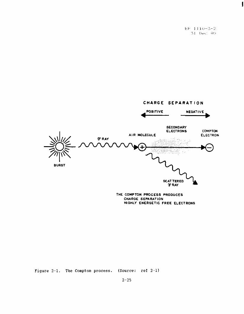
(2) Compton scattering. When the downward directed rays encounter the upper regions of the atmosphere, they begin to interact with the atoms (or moleculesE of the atmosphere at a rate which is a function of atmospheric density and burst conditions. The dominant interaction is Compton scattering, in which the energy of a gamma ray is partially transferred to an electron of an air atom (or molecule). The electron then begins traveling in approximately the same direction as the gamma ray. The other product of collision is a gamma ray of reduced energy. Figure 2-l illustrates this process (ref 2-l). The spherical shell of gamma rays is converted during Compton scattering into a spherical shell of accelerated electrons.

(3) Deposition region. The region in which Compton scattering occurs is called the deposition region. The thickness and surface range of the deposition region is a function of height-of-burst (HOB) and weapon size and type. A representative thickness is from 20 kilometers to 40 kilometers, but a deposition region may be as thick as 70 kilometers (lo-kilometer to 80- kilometer altitude) for a 300-kilometer HOB and a lo-megaton weapon.

(4) Radiating magnetic field. In the spherical shell of Compton electrons, the electrons are charged particles that rotate spirally around the Earth’s geomagnetic field lines (ref 2-2). The electrons thus have a velocity component transverse to the direction of the gamma radiation. These transverse currents give rise to a radiating magnetic field. This field propagates through the atmosphere to the Earth’s surface as if it were contained in the same spherical shell as that formed by the original gamma ray shell.

2 -2

F’ p’:s ., 1 ‘, (‘! :’ ;.

. . j j!Y,i -, I

b. HEMP ground coverage. Szgnificant HEMP levels can occur at the Earth’s surface out to the tangent radius (and beyond, for frequencies below 100 kilohertz). The tangent radius is where the line of sight from the burst is tangent with the Earth’s surface. If one assumes a spherical Earth of radius Re, the tangent radius Rt is given by--

(eq 2-l)

where HOB is the height of burst. For an approximate Earth radius of 6371 kilometers, an HOB of 100 kilometers corresponds to an Rt of 1121 kilometers, an HOB of 300 kilometers corresponds to an Rt of 1920 kilometers, and an HOB of 500 kilometers corresponds to an Rt of 2450 kilometers. Thus, the HEMP generated by a nuclear explosion at an altitude of 500 kilometers vuuld illuminate the whole continental United States. If high-yield weapons are used, the field strength will not vary much with HOB, so this large geographic area can be covered with little reduction in peak field strength.

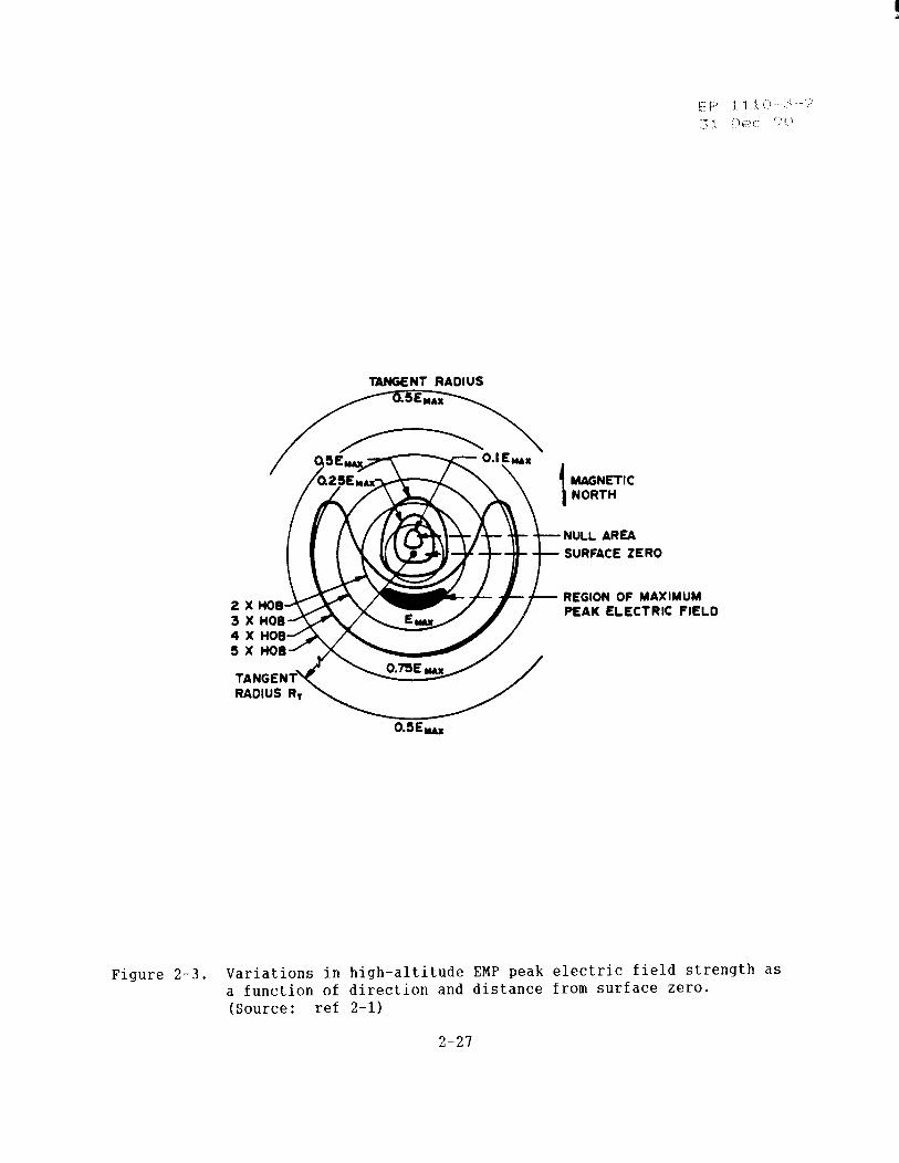
C. Field strengths versus ground location. HEMP fields can be significant out to the tangent radius, but the exact field strength as a function of ground position depends on many factors. Burst-observer geometry is important because HEMP is produced by electron motion transverse to the Earth’s magnetic field. Thus, electron moving along the field do not radiate, For a burst at high geomagnet,ic latitudes, as would be the case for Europe or North America, the pattern shown in figure 2-3 results. There will be a region of near--zero field strength north of the sub-burst point, where the magnetic field lines from the burst site intersect the Earth. There will also be a broad arc of maximum field strength that corresponds to electron trajectories perpendicular to the geomagnetic field. The field amplitude is an appreciable fraction of the peak amplitude (about 0.5 for most high--yield weapons) out to the tangent radius. The EMP field strenqth will also vary as a function of HOB, weapon yield (especially gamma yield), and geomagnetic field, which depends Oii geo- magnetic latitude. Near the equator, the Earth’s magnetic field strength is weaker and the orientation is very different, so peak HEMP fields would be smaller and the field strength pattern much different than that shown.

d. Electric field. A commonly used unclassified tLrre waveform of d lIEMP electric field E(t) in free space can be approximated by the analytical expression--

E(t) = kEpke aft -ts)

* (kV/m) _ __--- .---- lte (a+b) (t-t,)

leq 1 2-. 2

p: ! , 1 1 .! ,, / :!, <.’

::,:I j,,,(.:,,,: -y.:,, I

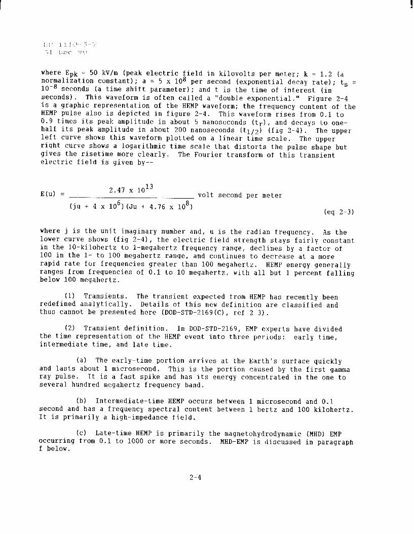
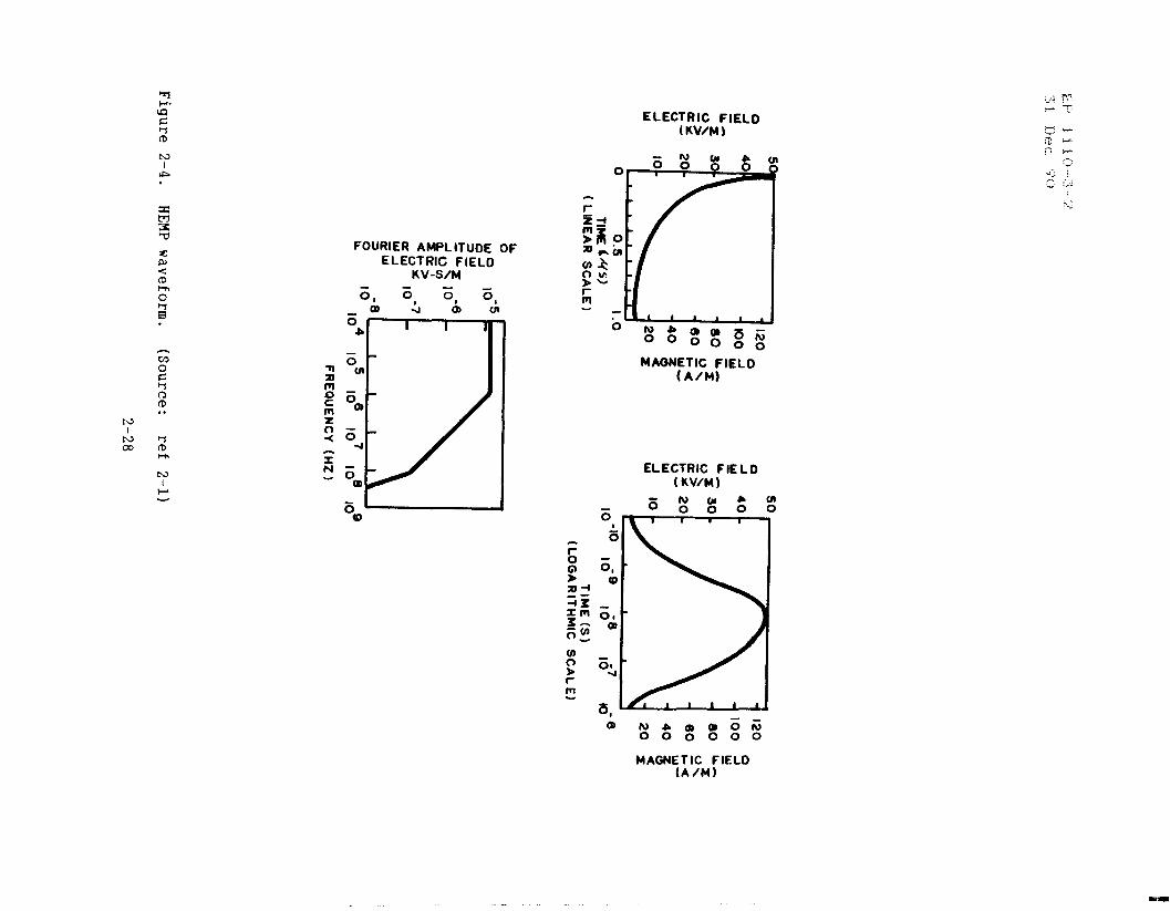
where Epk = 50 kV/m (peak electric field in kilovolts per meter; k = 1.2 (a normalization constant); a = 5 x lo* per second (exponential decay rate); t, = 10e8 seconds (a time shift parameter); and t is the time of interest (in seconds) a This waveform is often called a “double exponential.” Figure 2-4 is a graphic representation of the HEMP waveform; the frequency content of the HEMP pulse also is depicted in figure 2-4. This waveform rises from 0.1 to 0.9 times its peak amplitude in about 5 nanoseconds (tr), and decays to one- half its peak amplitude in about 200 nanoseconds (tl/2) (fig 2-4). The upper left curve shows this waveform plotted on a linear time scale. The upper right curve shows a logarithmic time scale that distorts the pulse shape but gives the risetime more clearly. The Fourier transform of this transient electric field is given by--

E(u) = 2.4’7 x 1013

volt second per meter

(ju + 4 x 106) (Ju + 4.76 x 108) (eq 2-3)

where j is the unit imaginary number and, u is the radian frequency. As the lower curve shows (fig 2-g), the electric field strength stays fairly constant in the lo-kilohertz to l-megahertz frequency range, declines by a factor of 100 in the l- to loo-megahertz range, and continues to decrease at a more rapid rate for frequencies greater than 100 megahertz. HEMP energy generally ranges from frequencies of 0.1 to 10 megahertz, below 100 megahertz.

with all but 1 percent falling

(1) Transients. The transient expected from HEMP has recently been redefined analytically. Details of this new definition are classified and thus cannot be presented here (DOD-STD-2169(C), ref 2-3).

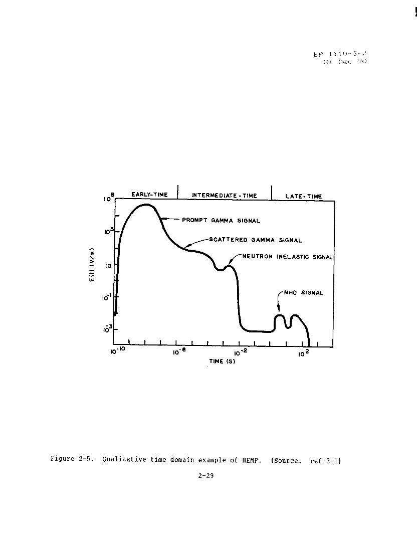
(2) Transient definition. In DOD-STD-2169, EMP experts have divided the time representation of the HEMP event into three periods: early time, intermediate time, and late time.

(a) The early-time portion arrives at the Earth’s surface quickly and lasts about 1 microsecond. This is the portion caused by the first gamma ray pulse. It is a fast spike and has its energy concentrated in the one to several hundred megahertz frequency band.

(b) Intermediate-time HEMP occurs between 1 microsecond and 0.1 second and has a frequency spectral content between 1 hertz and 100 kilohertz. It is primarily a high-impedance field.

(c) Late-time HEMP is primarily the magnetohydrodynamic (MHD) EMP occurring from 0.1 to 1000 or more seconds. MHD-EMP is discussed in paragraph f below.

2-4

(3) Qualitative characteristics. Figures 2-5 and 2-6 show unclassified qualitative HEMP characteristics.

f. Magnetohydrodynamic EMP (MHD-EYP) . MHD-EMP is the late time (t > 0.1 second) component of EMP caused by a high-altitude nuclear burst. Two distinct physical mechanisms are thought to produce different parts of the MHD-EMP signal: an “early phase” from 0.1 to 10 seconds after the detonation, and a “late phase” lasting from 0.1 to 1000 seconds. MHD-EMP fields have low amplitudes, large spatial extent, and very low frequency. Such fields can threaten very long landlines, including telephone cables and power lines, and submarine cables.

(1) MHD-EMP early-phase generation. A nuclear burst at high altitudes gives rise to a rapidly expanding fireball of bomb debris and hot ionized gas. This plasma tends to be diamagnetic in that it acts to exclude the Earth’s magnetic field from the inside of the fireball. Thus, as the fireball expands and rises in early stages, it will deform the geomagnetic field lines and thereby set up the early phases of the MHD-EMP, which can propagate worldwide. The region on the ground immediately below the burst is shielded from early- time MHD-EMP by a layer of ionized gas (the X-ray patch) produced by X-rays from the nuclear burst.

(2) MHD-EMP late-phase generation. Residual ionization and the bomb- heated air under the rising fireball are mainly responsible for the late phase of the MHD-EMP. As the bomb-heated air rises, residual ionization moves across geomagnetic field lines and large current loops form in the ionosphere. The ionospheric current loops then induce earth potentials. The late phase of the MHD-EMP is seen in large sections of the Earth’s surface, including regions at the magnetic conjugate points. Though amplitudes are smaller than for HEMP, the low-frequency fields can introduce damaging potential differences on long cable systems.

(3) Electronic surge arresters. The longer duration and greater energy content coupled into electrical lines in the DOD-STD-2169 environment is an important factor in the design and selection of electronic surge arresters.

2-3. Other EMP environments. Of several different kinds of EMP environments, HEMP is the one specified most often for system survivability. The discussion of HEMP applies to all systems that must survive a nuclear event, even though they are not targeted or even located close to a target. One reason is that the peak field amplitudes are large enough to damage or upset most unprotected electronic systems that use solid-state technology. Further, the frequency band is broad and thus all types of electronic/electrical systems are potentially susceptible. Third, as discussed previously, the HEMP area coverage is large. The fact that HEMP occurs when other nuclear environments are absent implies that systems with no defense against other nuclear effects may need protection against HEMP. Although HEMP is a vital concern for mission-critical systems and is the environment addressed in this manual,

2-5

other environments are briefly discussed for the sake of completeness. Table 2-l lists some of the other EMP environments and compares their properties.

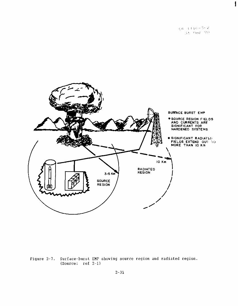
Surface burst EMP (SBEMP) SBEMP is produced by a nuclear burst close (leas; than 0.2 kilometer) to the-Earth’s surface (fig 2-7). The EMP is generated in the source region, which extends out to a radius of 3 to 5 kilometers from the burst. EMP environments inside the source region can affect systems such as ICBMs or command centers that have been hardened to withstand nuclear blasts, thermal energy, and radiation inside the source region. A surface burst also has fields radiating outside the source region, with those field amplitudes significant (greater than 5 kilovolts per meter) out to ranges of 10 kilometers and more. In t.his range, the radiated EMP is a principal threat to systems that respond to very low frequencies or have very large energy collectors such as long lines. Conducted EMP for these systems is such that special attention must be given to surge protection to ensure that the high currents can be dissipated.

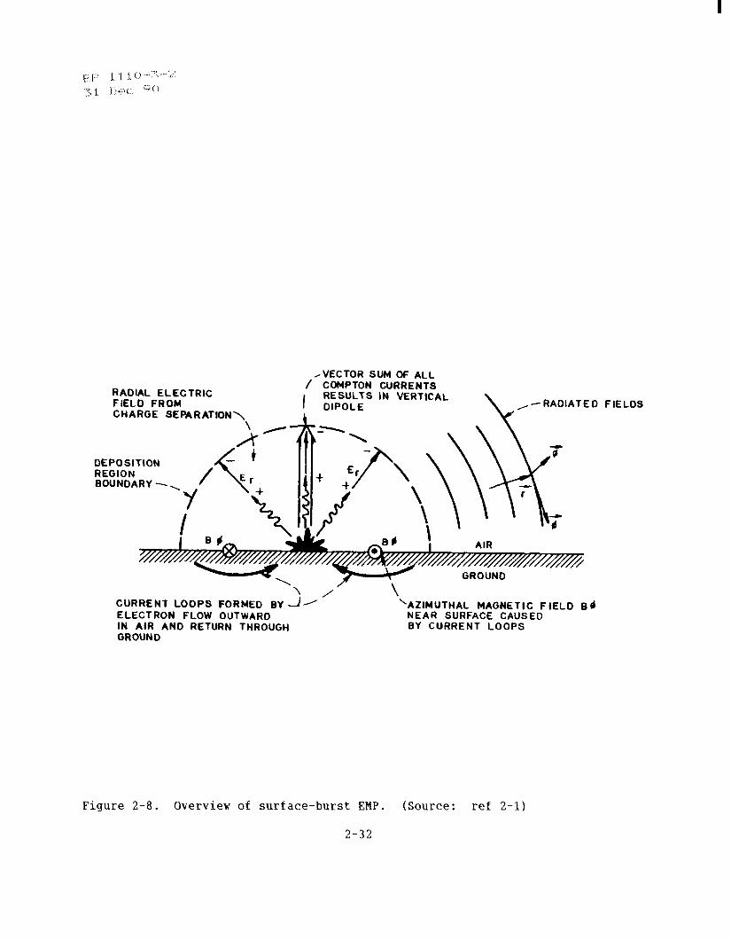
(1) Source region. The generation of EMP by a surface burst starts when the gamma rays travel out radially from the burst. These rays scatter Compton electrons radially, leaving behind relatively immobile positive ions (fig 2-8). This charge separation produces radial electric fields (Er) with amplitudes over 100 kilovolts per meter (amplitudes may approach 1 megavolt per meter) and risetimes as short as a few nanoseconds. Since the -ground conducts better than the air at early times, the strong radial electric field causes a ground current to flow in a direction opposite to the radial Compton current in the air. The resulting current loops produce azimuthal magnetic fields. Magnetic fields are strongest at the Earth’s surface and diffuse both upward and downward from the interface. The discontinuity due to the air- Earth interface also generates strong vertical electric fields in the source region. Source region fields depend strongly on factors such as weapon yields (gammas and neutrons), HOB, and distance from the burst. The interaction with a system is very complex: besides the EM fields, the system may be exposed to nuclear radiation, in addition to being located in a region of time-varying currents and conductivity. In specifying a source region environment for a system, then, the concept of balanced survivability is useful, as it is with all EMP environments. If a facility is designed to withstand ionizing radiation and other nuclear effects at a specified range from a given burst, it should also be designed to withstand the EMP effects generated at that range.

(2) Electric and magnetic field relationship. The time-varying currents and conductivity of the surface-burst source region imply a complex relationship between electric and magnetic fields, which does not show the simple magnitude and direction relationships of a plane wave. Determination of these relationships is beyond the scope of this manual.

(3) Radiated region. Outside the source region, the most important feature of the charge distribution produced by a surface burst is the asymmetry due to the air--earth interface (fig 2-R). In an infinite uniform

2-6

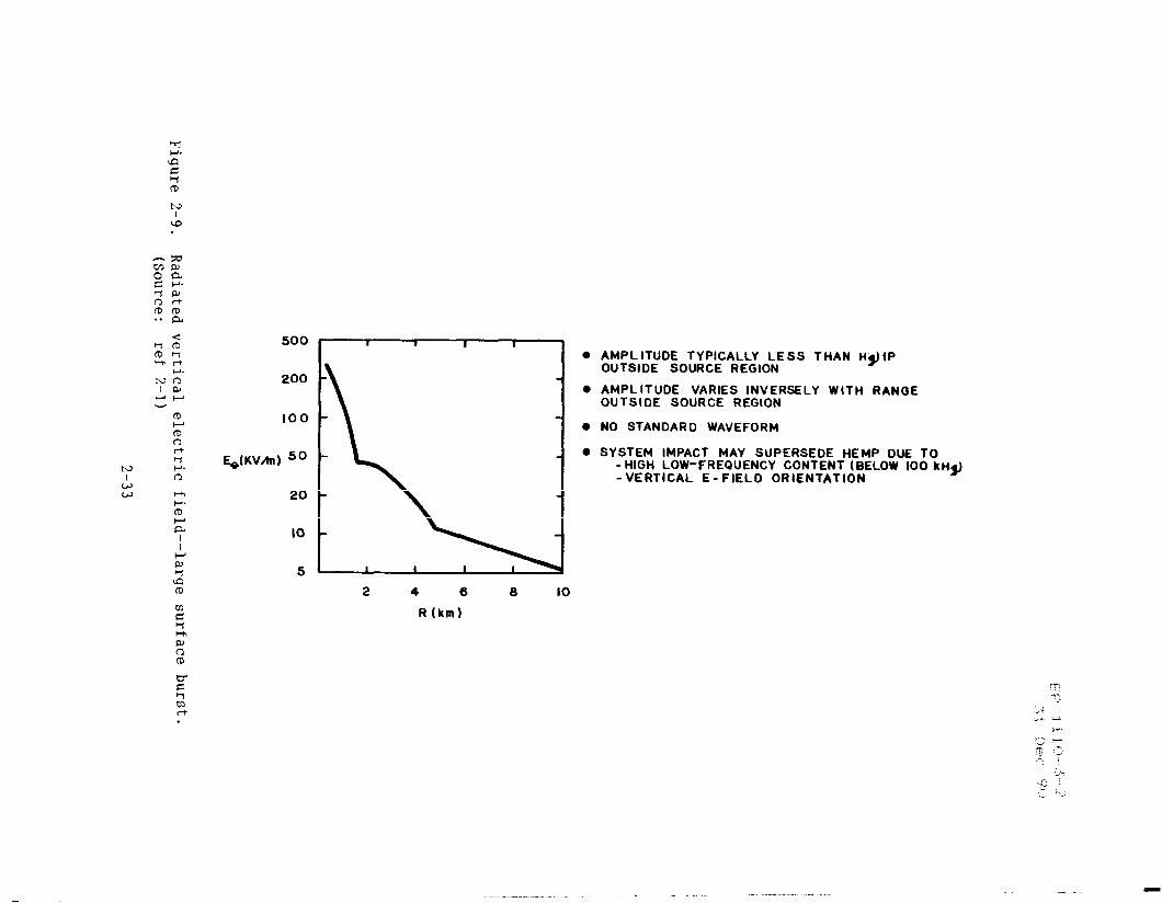
atmosphere, Compton electrons would travel out radially in all directions. However, for SBEMP, the earth interferes with down-flowing electrons, which results in a net vertical flow of Compton current. This produces a tirne-vary- ing vertical dipole that radiates outside the source region. The main components of the radiated field are the vertical electric field and the azimuthal magnetic field.The field amplitude has a l/R dependence with range, as is typical of electric dipole radiation. The field rises quickly to its first peak [electric field vector vertically upward), with a second peak of opposite sign following some tens of microseconds later. More of the energy occurs at lower frequencies than for HEMP. Figure 2-9 shows the calculated electric field amplitude as a function of range for a large surface burst. As the figure shows, radiated surface burst field amplitudes most often are smaller than HEMP fields outside the source region. However, field amplitudes can still. be significant at ranges of 10 kilometers or more. The riqht portion of the curve shows the inverse relationship between amplitude and range beyond 5 kilometers. This is typical of electric dipole radiation in the far-field region. There is no standard waveform as there is for HEMP. Thus, the very concept of a standard waveform is less likely to be useful for SBEMP because of the variation in amplitude and waveform with range and weapon yield (output) . Radiated SBEMP typically gives off most of its energy at lower frequencies (below 100 kilohertz). The increase in low frequency content and the vertical electric field orientation mean that the system impact of radiated SBEMP may be more important than that of HEMP for some systems, even though HEMP field magnitudes are generally larger.

b. Air-burst EMP.

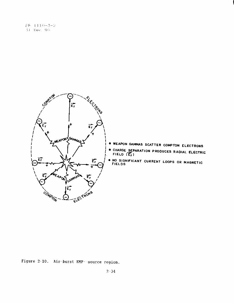
(1) Source region. Air-burst EMP results from a nuclear explosion at intermediate altitudes--2 to 20 kilometers. The EMP produced by a burst at heights between 0.2 and 2 kilometers will share characteristics of air and surface bursts, and a burst between 20 and 40 kilometers will cause EMP sharing characteristics of air-burst and high-altitude EMP. The source region resembles the surface-burst source region in that weapon gammas scatter Compton electrons radially outward (fig 2-10). Positive ions are left behind, producing charge separation and radial electric fields. For ai.r-burst EMP, there is no return path through the ground. Due to ionization, however, increased air conductivity enables a conduction current to flow opposite the Compton current in the air. Still, no significant current loops are formed, and the large azimuthal magnetic fields typical of a surface burst do not result.

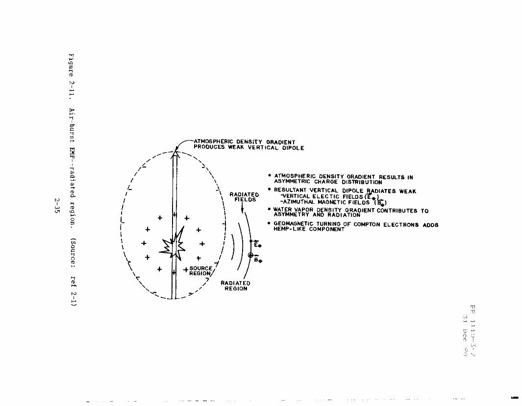
(2) Radiated region. Outside the source region, the radial charge separation resulting from the Compton current will produce some radiated fields because a slight asymmetry exists. At intermediate altitudes, the atmospheric density gradient permits Compton electrons to move farther up than down. This asymmetry results in electric dipole radiation (fig 2-11). The water vapor density will also vary with height, though this variation depends on the weather. A typical decrease in water vapor density with altitude will reinforce the asymmetry produced by the atmospheric density gradient. Even

2-7

with these two effects combined, the asymmetry is much weaker than for a surface burst. The typical field strengths produced are on the order of 300 volts per meter at 5 kilometers from the burst. Pulse waveforms vary significantly with burst altitude and assumed water vapor gradient, with typical risetimes in the l- to 5-microsecond range. The recoil Compton electrons can also produce a radiated signal by the same geomagnetic turning mechanism that gives rise to HEMP. This is called magnetic dipole radiation. At low altitudes, electron paths are short so that peak amplitudes are limited to hundreds of volts per meter, mainly to the east and west of the burst. The peak amplitude increases with burst height until it reaches tens of kilovolts per meter as the burst approaches the high-altitude region. Rise and decay times are similar to those for HEMP--on the order of tens of nanoseconds.

C . System generated EMP (SGEMP) . SGEMP results from the direct interaction of nuclear weapon gammas and X-rays with the system. Because weapon gammas and X-rays are attenuated by the atmosphere at low altitudes, SGEMP has special importance for systems outside the atmosphere, such as satellites in space and missiles in flight. These can receive significant gamma and X--ray exposures at considerable distances from a nuclear burst. SGEMP involves complex modes of field and current generation that strongly depend on the system's physical and electrical configuration. As a result, there is no standard threat. The field amplitudes generated can be as large as 100 kilovolts per meter, making SGEMP a significant threat to exposed systems.

(1) Coupling modes. The initial physical process is the generation of energetic free electrons by Compton and photoelectric interactions of weapon X-rays and gammas with the system materials. Emitted electrons produce space- charge fields that turn back later electrons or, at higher gas pressures, cause appreciable ionization. Emission of the electrons from internal walls results in current generation and, hence, EM fields inside cavities. This effect is termed internal EMP (IEMP). Coupling occurs both by electric and magnetic field coupling directly onto signal cables and by induced current flow on cable shields and ground systems. The asymmetric displacement of electrons from a cable shield and from internal conductors and dielectrics inside a single cable or cable bundle produces a distributed current generator over the whole exposed region of the cable. Electron emission from the outer skin of the subject system generates whole body interaction effects that produce charge displacement and direct field coupling. These effects also can influence internal EMP if there are penetrations or openings to the inside.

(2) Transient radiation effects on electronics. The direct impingement of radiation (e.g., X-rays, gamma rays, neutrons) can also change the performance of semiconductor electronics through atomic interactions. Operating thresholds, junction voltages, and the crystalline structure of solid-state materials can be affected, thus changing the way devices and cir- cuits using such materials operate. TREE normally is important only when modern electronics might be exposed to the nuclear detonation source region with a high in-flow of nuclear radiation.

2-8

d. Summary e Table 2-2 out lines the EMP waveforms important for cr itical systems. HEMP is the most difficult threat to harden against because of its large spatial extent, high amplitude, and broad frequency coverage. It is also the simplest threat to describe using the waveform definition in equation 2-2 and the plane wave approximation. The source region for an air or surface burst combines intense fields with significant time-varying conductivities and environments. Source-region EMP is important for systems that can withstand other nuclear environments present in the source region. EMP radiated from a surface burst usually has lower amplitude than HEMP and can affect systems more due to the vertical field orientation and lower frequency. Air-burst radiated fields have lower amplitudes and are less likely to be important (a system hardened to survive HEMP will survive radiated air-burst EMP). SGEMP is characterized by very high amplitudes, very fast risetimes, and importance to systems outside the atmosphere. MHD-EMP has low amplitude but can damage the interface circuits of long landlines or submarine cables.

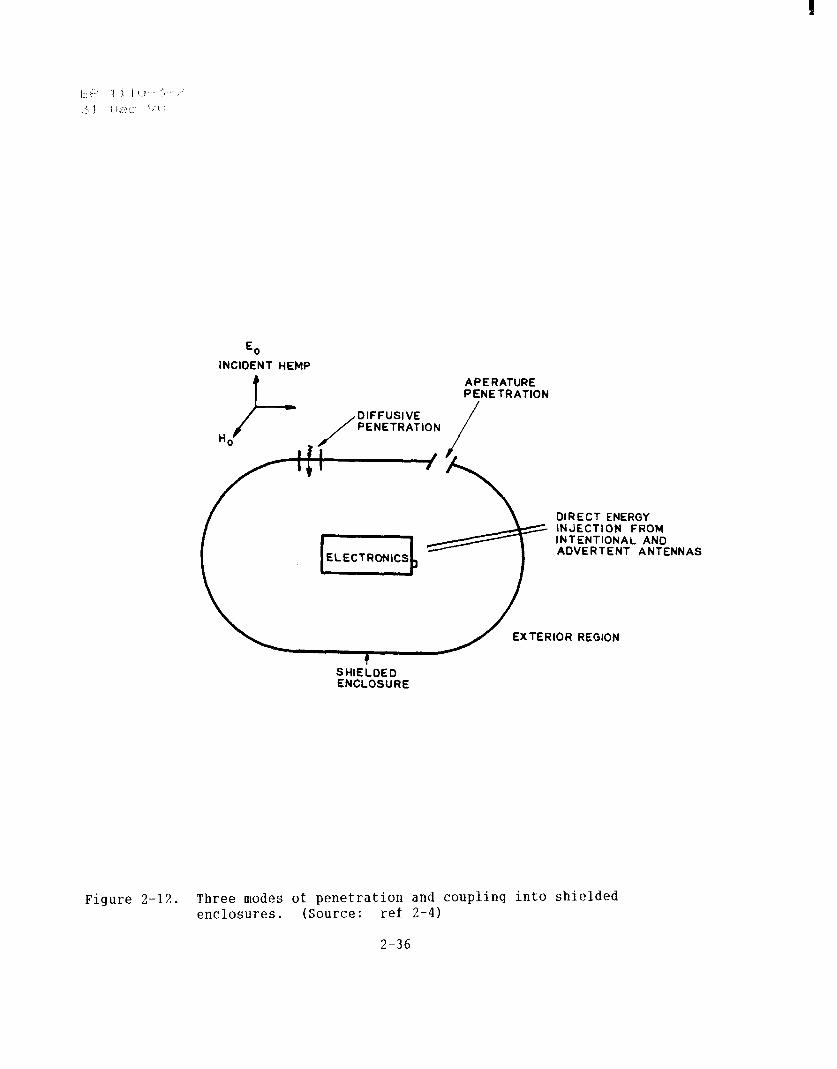
2-4. Environment-to-facility coupling. To analyze how HEMP will affect facilities and electronic equipment, the exterior free field threats must be related to system, subsystem, and circuit responses. The functional relationship between external causes and internal effects is often called a “transfer function.” The analysis involves learning how the system collects energy from the incident HEMP field. The result is usually a matrix of internal fields and transient voltages and currents that may flow in circuits and subsystems. This is called a “determination of the coupling interactions between the external threat and the system." Generally, HEMP enters shielded enclosures by three different modes: diffusion through the shield; leakage through apertures such as seams, joints, and windows; and coupling from inten- tional or inadvertent antennas. These different modes are shown in figure 2- 12 and are discussed next.

a. Modes of HEMP entry.

(1) Diffusion through the shield. HEMP fields diffuse through imperfectly conducting walls of shielded enclosures. The diffusion is greatest for magnetic fields and is a low-pass filtering event, as shown by the magnetic shielding effectiveness curve for an ideal enclosure (fig 2-13). Thus, the field that reaches the inner region of a shielded enclosure is basically a low-frequency magnetic field. This effect is greatest in an enclosure with solid metal walls. It is also seen somewhat in enclosures with metal rebar or wire mesh reinforcement. The shielding effectiveness (SE) for an enclosure with rebar is also shown in figure 2-13. The reduced SE at high frequencies for rebar and wire mesh structures allows a significant fraction of the incident HEMP environment to penetrate to electronics inside the enclosure.

(2) Leakage through apertures. Openings and other shielding compromises include doors, windows, holes for adjustments and display units, seams, improperly terminated cable shields, and poorly grounded cables.

2-9

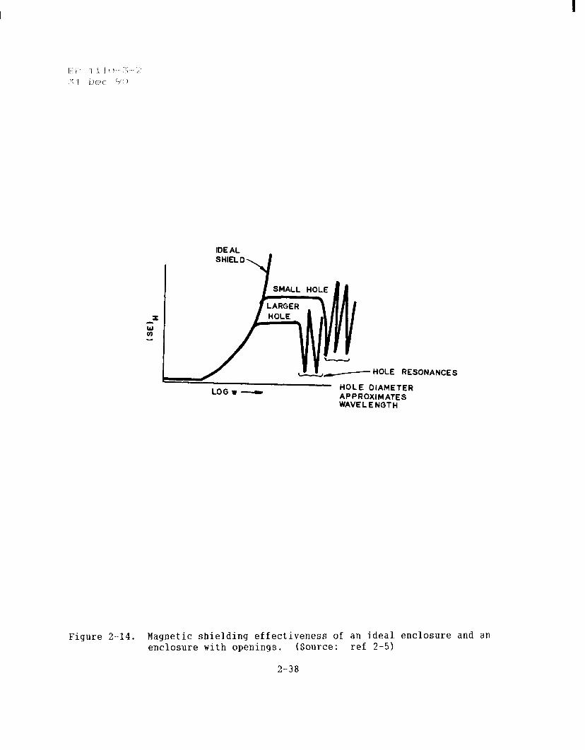
Unless properly treated, each opening is a leak through which the HEMP field can couple directly into the shielded enclosure. Leakage through an aperture depends on its size, the type of structure housing it, and its location. The aperture responds to both total magnetic and electric fields at the site of the leak. The effect of apertures on the magnetic SE of an ideal enclosure is shown in figure 2-14.

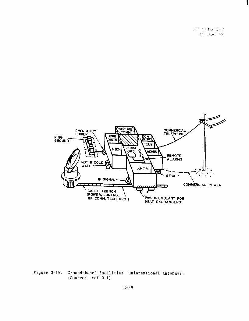
i3) Intentional and inadvertent antennas. Intentional antennas are designed to collect EM energy over specified frequency bands. However, there will also be an out-of-band response to HEMP. Because the incident HEMP field has a broad frequency spectrum and high field strength, the antenna response must be considered both in and out of band. Analytical models are available for determining the different antennas’ responses to HEMP. These models, along with the incident field, yield the HEMP energy that appears at the con- necting cable. This energy later reaches the electronic systems inside the enclosure at the other end of the connecting cable. Inadvertent antennas are electrically conducting, penetrating external structures, cables, and pipes that collect HEMP energy and allow its entry into the enclosure. As a rule, the larger the inadvertent antenna, the more efficient energy collector it is in producing large, transient levels in the enclosure. Figure 2-15 shows some inadvertent antennas for a ground-based structure. The coupling for inadver- tent antennas can be analyzed using transmission line and simple antenna models. These analyses, however, are complex and beyond the scope-of this manual. The reader is directed to references 2-2 and 2-6 for guidance on these analyses.

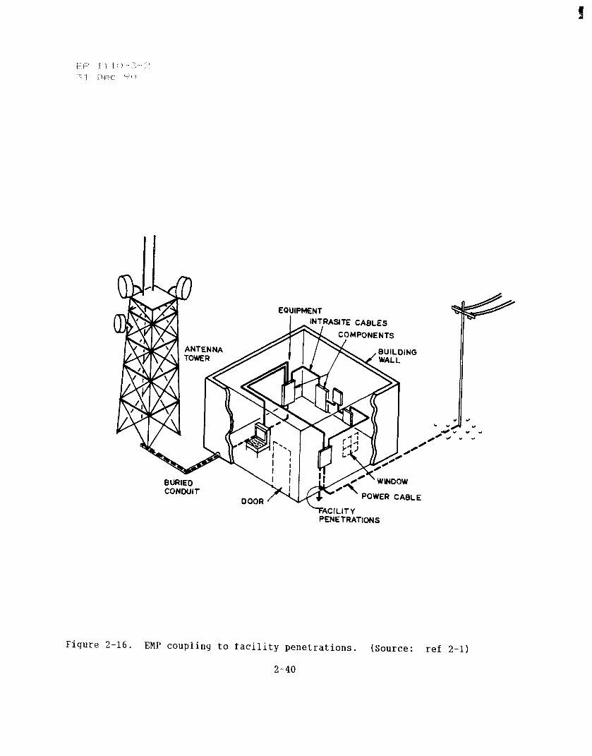
b. Conductive penetrations. Many factors affect the coupling of EM energy to penetrating conductors. The EMP waveform characteristics, such as magnitude, rate of rise, duration, and frequency, are each important. Further, the observer’s position with respect to the burst is a factor. Because the interaction between fields and conductors is a vector process, the direction of arrival and polarization is also important. Conductor character- istics also affect HEMP coupling. These include conductor geometry (length, path, terminations, distance above or below the earth’s surface), physical and electrical properties that determine series impedance per unit length (including diameter, resistivity, and configuration), and the presence and effectiveness of shielding. For overhead or buried conductors, the electrical properties of soil affect coupling. Though dielectric permittivity and magnetic permeability may be significant, soil conductivity is usually the greatest determining factor for coupling. This is because both HEMP attenuation in the ground and reflection from the ground increase with greater soil conductivity. The soil skin effect also varies. An EM wave in a conduc- tive medium ttenuates to 0.369 of its initial amplitude in a distance d = (2/pwc) l/8 where d is the skin depth, p is the magnetic permeability of the medium, w’ is the angular frequency, and c is the conductivity. Because the skin depth is greater at lower frequencies, lower frequency field components attenuate less and the pulse risetime increases. Many elements of a facility can act as efficient collectors and provide propagation paths for EMP energy. As shown in figure 2-16, EMP can couple to structures such as

2-10

power and telephone lines, antenna towers, buried conduits, and the facility grounding system. Actual antennas, nonelectrical penetrators such as waterpipes, and any other conducive penetration can couple EMP energy into a structure. In addition, if the structure is not shielded or is not shielded well enough, EMP can couple to the cables between equipment inside. Paragraphs (1) through (3) below briefly describe coupling mechanisms, including theory, and give rough values for the currents and voltages that can arise from a typical EMP event.

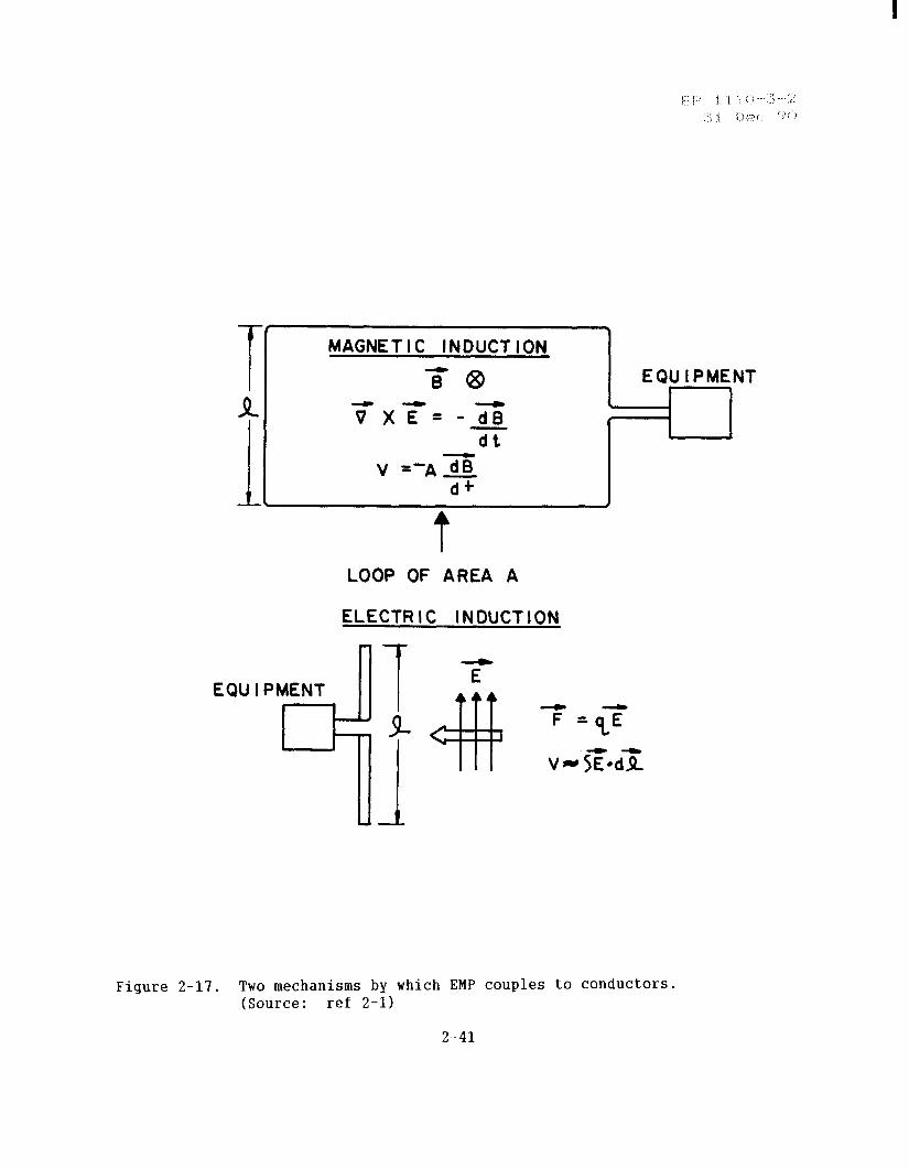
(1) Basic coupling mechanisms. Figure 2-17 shows two basic modes by which currents and voltages are induced in conductors. One mechanism shown is that for inducing voltage in conductors by electric field. The electric field exerts forces on the “mobile” electrons in the conductor, which results in a current. The voltage associated with the force is the integral of the tangen- tial component of E along the length of the wire. This assumes the electric fieldis constant over the length of the wire and is parallel to it. The other mechanism by which currents are induced on conductors is through changes in the magnetic field, also shown in figure 2-17. Faraday’s Law is the mathe- matical expression that describes this phenomenon. This law relates the time rate of change of the magnetic field to the production of an associated electric field. This electric field “curls” around the changing magnetic field and causes a voltage if a loop is present. The voltage for the loop of area A in the figure is V = A(dB/dt), where B is normal to the loop and has the same magnitude over the whole loop. This can give a good approximation with HEMP when the magnetic field can be considered uniform over the area of the loop. The fast rise rate of the magnetic field can produce large currents and voltages. A sample calculation is helpful. Assume the following--

A = loop area = 0.1 meter squared (m2)

E(t) = Ce-t’a where C = 50,000 volts/meter

a = 0.5 x lo6 (time constant)

(Note: a simple exponential is used for this example.)

H = E/377 (a plane wave)

- e-t’a(C/377) -.~

U = u. (loop antenna in free space)

U 0

= 4(pi) x 1O-7 Webers/amp-meter

Then :

= 50,000/377 eet’Oe5 ’ lo -6

H amps/meter

= 132.6 e -t/o.5 x lo6

amps/meter

2-11

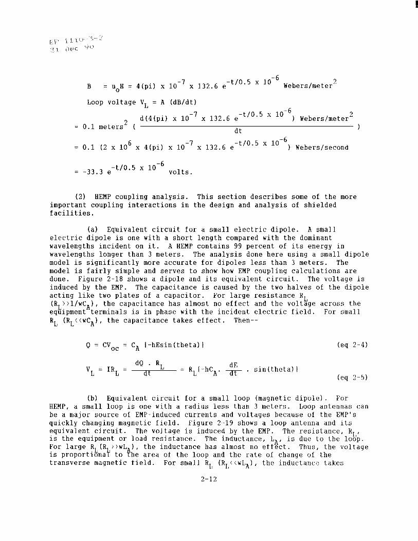
B = u,H = 4(pi) x 10 -7

x 132.6 e -t’0*5 ’ lov6 Webers/meter2

Loop voltage VL = A (dB/dt)

d(4(pi) x 10 -7

= 0.1 meters2 ( x 132.6 e

-t/0.5 x lo6 1 Webers/meter2

dt 1

= 0.1 (2 x lo6 x 4(pi) x 10e7 x 132.6 e -t/o.5 x 1o-6

) Webers/second

= -33.3 e -t/0.5 x lo+ volts

.

(2) HEMP coupling analysis. This section describes some of the more important coupling interactions in the design and analysis of shielded facilities.

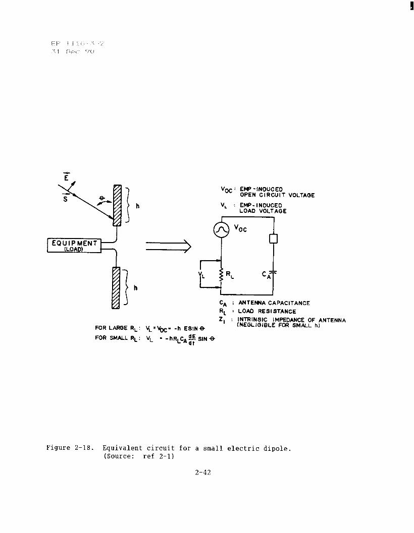
(a) Equivalent circuit for a small electric dipole. A small electric dipole is one with a short length compared with the dominant wavelengths incident on it. A HEMP contains 99 percent of its energy in wavelengths longer than 3 meters. The analysis done here using a small dipole model is significantly more accurate for dipoles less than 3 meters. The model is fairly simple and serves to show how EMP coupling calculations are done. Figure 2-18 shows a dipole and its equivalent circuit. The voltage is induced by the EMP. The capacitance is caused by the two halves of the dipole acting like two plates of a capacitor. For large resistance RL (RL)>l/wCA), the capacitance has almost no effect and the voltage across the equipment terminals is in phase with the incident electric field. For small RL (RL(<wCA), the capacitance takes effect. Then--

Q = CV oc = CA (-hEsin(theta) 1 (eq 2-4)

dQ . RL VL IRL dt~ RLI-hCA. . f

2-5)

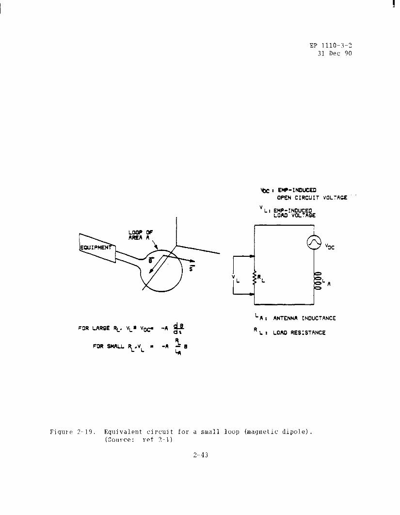
Equivalent for small (magnetic For a loop one a less 3 Loop can

a source EMP-induced and because the quickly magnetic Figure shows loop and equivalent The is by EMP.

the or resistance. resistance,

For RL(Rk))wLt), inductance, is to loop.

inductance almost effect. the is to area the and rate change the

magnetic For RL the takes

, j. /I..J j , \ ( ! .:: /.... ,,:

..!, ‘, (,!pf” ‘..;s :I

effect and the current in the loop is proportional to the magnetic field. The current will flow in a way that makes the magnetic flux through the loop due to the current cancel the magnetic flux through the loop due to the field.

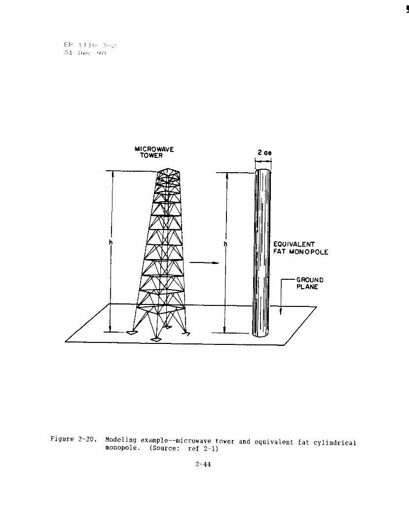
(c) Typical coupling model. In actual coupling calculations, it is often hard to depict a structure using the small dipole circuits just described. For example, the microwave tower in figure 2-20 is not small compared to a 3-meter wavelength, and it would be hard to represent it by superimposing loops of different sizes, shapes, and orientations. Instead, such a structure can be electrically approximated by a monopole of the same height and of some effective radius, a,. An upper bound on the effective radius is given by the tower dimensions at the base. The effect of ground is approximated by assuming an infinitely conducting ground plane. For a worst- case vertical orientation, the equivalent fat monopole over an infinitely conducting ground plane is equal to a dipole of the same radius and twice the height in free space. Models such as this can be used to find bounds or orders of magnitude for coupling to large or complex structures. Model validity or accuracy depends on the amount and kind of approximation used and on how well results agree when compared empirically with experimental or complex analytical data.

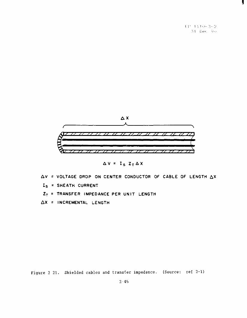
(d) Shielded cable coupling. To analyze the transients induced on cables by EMP, two calculations usually are needed to find the coupling onto the cable sheath and the voltage and resultant currents induced on the internal wires. The calculation of coupling onto the cable sheath depends on cable construction and location, and will be discussed for some typical cases later. Figure 2-21 shows the calculated voltage induced on a wire inside a shielded cable. The transfer impedance can be found theoretically, especially for simple cable shields such as solid metallic conduits. For example, the transfer impedance of a thin-walled tubular shield is given by--

1 (l+j)T/d ZT = . (eq 2-6)

2 (pi 1 rcT sinh(l+j)T/d

where r is the radius of the shield, c is its conductivity, T is the wall thickness, j is the unit imaginary number, and d is the skin depth. Some geometries, however, such as braided coaxial cables, are too complex for theoretical treatment. Thus, it is often preferable to determine the transfer impedance by experiment. For braided coaxial cables, the transfer impedance is typically expressed as--

ZT = R. ( (ltj's'd- ) = jwME

sinh(l+j)s/d (es 2-7)

where R, is the d.c. resistance per unit length, j is the unit imaginary number, s is the shield wire diameter, d is the skin depth, w is the angular frequency, and Ml2 is the leakage inductance per unit length. For typical

2-13

braided coaxial cables, R, ranges from 1 to 25 milliohms per meter and Ml2 ranges from 0.1 to 1 nanohenry per meter. At low frequencies, s/d (< 1 and wMl2 (( R, and ZT reduces to R,. For example, for an RG-58 coaxial cable at f = 104hertz, d = 0.24 << 1 and wMl2 = 0.01 milliohms per meter (( R, = 14.2 milliohms per meter so the transfer impedance is about equal to R,. A 500-amp current on a cable length of 100 meters will therefore induce a voltage drop on the center conductor of 500 amps(100 meters) (14.2 milliohms per meter) = 710 volts.

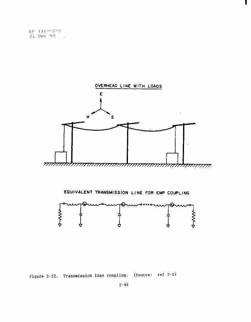
(e) Transmission line coupling. Transmission line theory is the chief method used to calculate EMP coupling to aerial and buried conductors, simple cables, and other long penetrators (e.g., pipes, ducts). A transmission line picks up EMP from both the electric field and the changing magnetic field. The loop formed by the line, its terminations, and the ground behaves much like a loop antenna and picks up EMP from the transverse changing magnetic field. The links between the line and ground behave much like dipole antennas and pick up EMP from the vertical electrical field. The line also picks up EMP from the longitudinal electric field. Though this last source seems the most clearcut, it does not cause as much of the total current and voltage as the other two. The transmission line theory involves many points that were ignored in the analyses of small dipole and loop antennas. First, the conductor is long compared to the incident wavelengths. This means that currents and voltages will differ everywhere on the line. Also, there will be reflection from the ground plane. With all such factors taken into account, an analytical solution can be, obtained, often with the help of a computer. This solution usually involves the short circuit current and the open circuit voltage at the line’s termination. Figure 2-22 shows an approximate model of this EM coupling. The transmission line is broken into N sections. N is chosen based on the bandwidth needed in the model. One- to three-foot sections are typical. Each inductor and capacitor in the model is chosen such that L = Z,T/2 and C = T/Z,, where Z, is the characteristic impedance and T is the transit time in each section. The voltage source in each section depends on the incident fields. This theory also applies to transmission lines with multiple cables. In this case, a source and load impedance will exist between each cable and ground and between each cable and every other cable. Current and voltages will be induced between the cables. This is caused by the changing magnetic field component transverse to the loop formed by two cables and by the electric field component pointing between them. This kind of EMP pickup is called the differential mode. EMP pickup causing currents and voltages between each cable and ground is called the common mode. These two modes are often treated separately and both create a need for protection.

(f) Aerial conductors. Long, straight, horizontal aerial conductors include pole-mounted power distribution lines and signal-carrying cables. Figure 2-23 shows how the peak coupled current and the time-to-peak depend on the line length. The peak current and time-to-peak also depend on the line’s height above ground, its size and construction, the soil conductivity, and other factors. The figure shows peak currents calculated for a pulse of the form Eoewt/xl where E, is the peak field amplitude of 50 kilovolts per meter

2-14

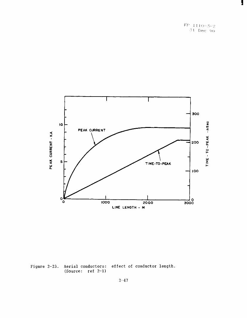
and x is an exponential decay constant of 250 nanoseconds. This waveform looks much like the standard double exponential discussed earlier. It is used here to make calculations easier. Grazing, end-on incident is assumed with a polarization of about 16 degrees from the horizontal. The vertical field component for this polarization angle is 15 kilovolts per meter. The horizontal field component is much larger (about 48 kilovolts per meter), but it gives rise to a smaller induced current because of transmission line behavior. This polarizat.ion is typical of that expected at latitudes in the United States where the magnetic dip angle is more vertical than horizontal. A worst-case angle of incidence is assumed. Figure 2-23 shows how peak current as a function of the line length approaches a limiting value, in this case about 10 kiloamps. The point at which the limiting value is reached is called the critical line length. The time required for the current to reach its peak value also increases with line length until a limiting value is reached. Figure 2-23 also shows the bulk current that will be induced on the aerial conductor. If the conductor is a shielded cable, the values shown will correspond to the sheath current. The currents induced on conductors inside the shield will depend on the transfer impedance.

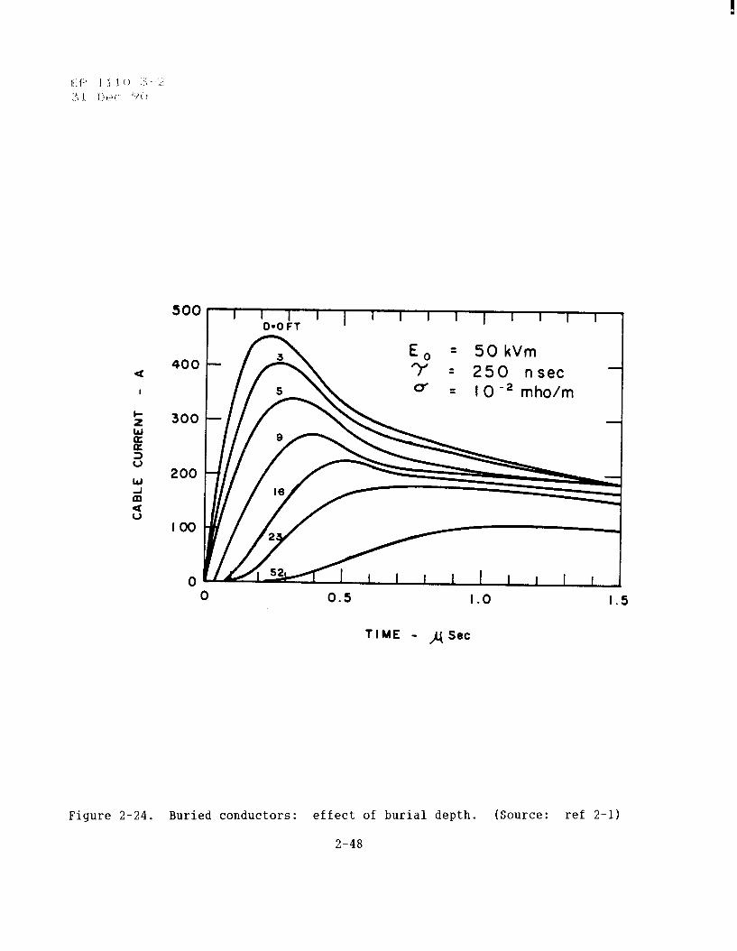
(g) Buried conductors, Buried conductors can be significant EMP collectors because low-frequency components of EMP fields are not greatly attenuated for typical soil conductivities and burial depths. The amplitude of the induced current varies inversely with the square root of the soil conductivity, which ranges from 10-4 to 10-2 mhos per meter. Figure 2-24 shows the variation in induced cable current with burial depth. The effect of deeper burial is both to reduce the amplitude of the induced current and to increase the risetime to peak current because of increased skin depth. (See para 2-4b above.) Figure 2-24 is for a semi-infinite cable. A finite cable will show a different response, especially near the cable ends. The differences in response are related to the cable sheath material and the way the cable is grounded. The cable’s induced current also depends on the amplitude, waveform, and direction of the incident pulse. It will be proportional to the amplitude of the incident pulse (Eo). It will also be proportional to the square root of the decay time constant (T) of the incident pulse for an assumed exponential waveform E(t) = Eoe-t/T. This constant is nearly the same as beta in the standard double exponential waveform. In the figure, the pulse is incident from directly overhead with the electric field parallel to the cable. This is a worst-case orientation. The current given in the figure corresponds to the total current induced on the cable, mainly

sheath current, that can be related to the current on conductors inside the shield in terms of the transfer impedance.

(h) Ringing. As discussed earlier, the incident HEMP pulse is a broadband signal with a time waveform approximated by very fast risetime and exponential decay. If all coupling paths had broadband frequency responses, EMP-induced transients would show similar waveforms. However, inductance, capacitance, and resistance are inherent in any cable, cable shielding, and grounding system, and give rise to frequency dependence. Any LRC system will

have characteristic resonant frequencies. EMP-induced transients thus will

2-15

tend to oscillate, or “ring,” at these dominant frequencies, with the decay rate of the oscillation ruled by the width gf the resonance in the frequency domain (fig 2-25) . A very narrow resonance can cause a long-lived oscillation. This increased energy is added to the system and the likelihood of damage increases. Typical ringing frequencies range from 1 to 15 mega- hertz, depending on the physical and electrical details of the shielding and grounding systems.

(i) Conductive penetrations. Pipes and other penetrators with nonelectrical functions act very much like the shield of a shielded cable. Most often such penetrators are buried. For these buried conductors, transmission line theory can be used to calculate HEMP coupling, with the soil acting as the return path. Both nonelectric penetrators and components with an electrical function can couple EMP energy by acting in a mode other than that for which they were designed. For example, waveguides usually are designed to guide waves of a much higher frequency than HEMP; however, currents can be coupled onto the exterior of waveguides and conducted to the sensitive equipment. Conductive penetrations not only can collect HEMP energy, they also can serve as low-impedance paths to ground for currents induced elsewhere in a facility.

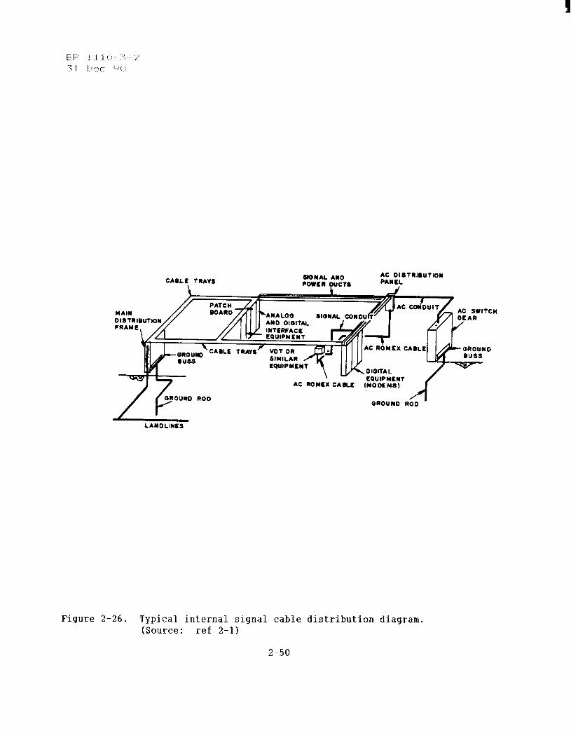
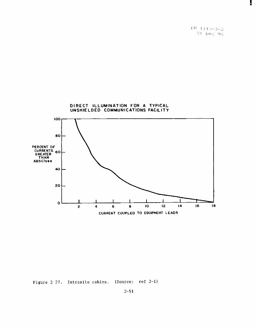
(3) Intrasite cables. Intrasite or internal cables at a structure may connect to mission-essential equipment. EMP-induced transients on these cables result partly from direct interaction with EMP fields that reach the structure’s interior. These internal EMP fields couple to long, internal cable runs and internal cable loops (fig 2-26). EMP-induced transients on internal cables may also result from “cross talk.” Typically, a cable that penetrates a facility will branch into many smaller cables (e.g., low-current power cables, individual telephone lines). These penetrators run alongside other internal cables so that penetrating EMP-induced transients tend to be shared. This especially occurs when cables run together in the same cable tray or conduit, but it can also happen to some degree if the cables pass within a few meters of each other. The result is that all cables linked to a piece of mission-essential equipment must be seen as potential sources of harmful voltage and currents. Figure 2-27 shows the distribution of currents at equipment leads for a typical unshielded telephone communications facility when subjected to a 50-kilovolt per meter EMP, polarized 16 degrees from the horizontal and coming from a worst-case direction. The structure has an incoming power line on which a peak current of 4 kiloamps is seen. Nineteen waveguides with a total peak current of 5 kiloamps also penetrate the structure. The waveguides come from a microwave tower and are grounded as they enter the structure.

2-5. Equipment susceptibility. System damage or upset from EMP is caused by currents and voltages induced in conductors exposed to a free-field or a

‘The narrow resonance results from circuits of high Q (quality factor) which have low resistive dissipation of energy.

2-16

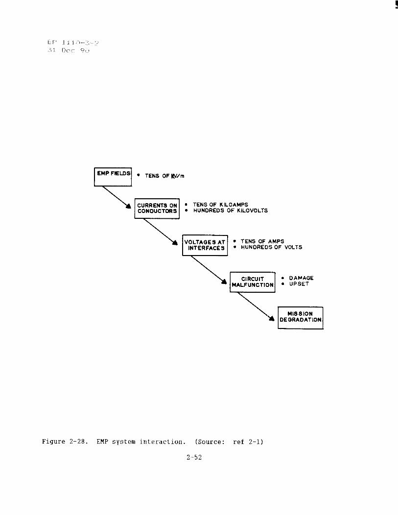
partly attenuated EM pulse coupled to circuits. External conductors, structures, and internal conductors act as unintentional receiving antennas and “coupling” paths. They can deliver the resulting EMP-induced currents and voltages to sensitive components of electronic equipment. The HEMP-induced currents on exterior long-line penetrators, such as power and telephone lines, can have amplitudes as high as thousands of amperes. Currents induced on internal cable runs can be as high as hundreds of amperes for most structures and even higher in facilities with lower SE. It is important to note that exterior voltage transients can be in the megavolt range, and it would be normal to expect an order of thousands of volts from internal coupling. Transients of these magnitudes can be delivered to electronic circuits, such as integrated semiconductor circuits, which can be damaged by only a few tens of volts, a few amperes, or less. These circuits also operate at relatively low levels (e.g., 5 volts and tens of milliamperes) and can be upset by EMP currents of similar values. If the large exterior coupled transients were allowed to enter a structure that had no HEMP protection treatment, even relatively “hard” devices, such as relay coils and radio frequency interference (RF11 filters, would likely be damaged. Figure 2-28 shows this potential EMP interaction leading to mission degradation.

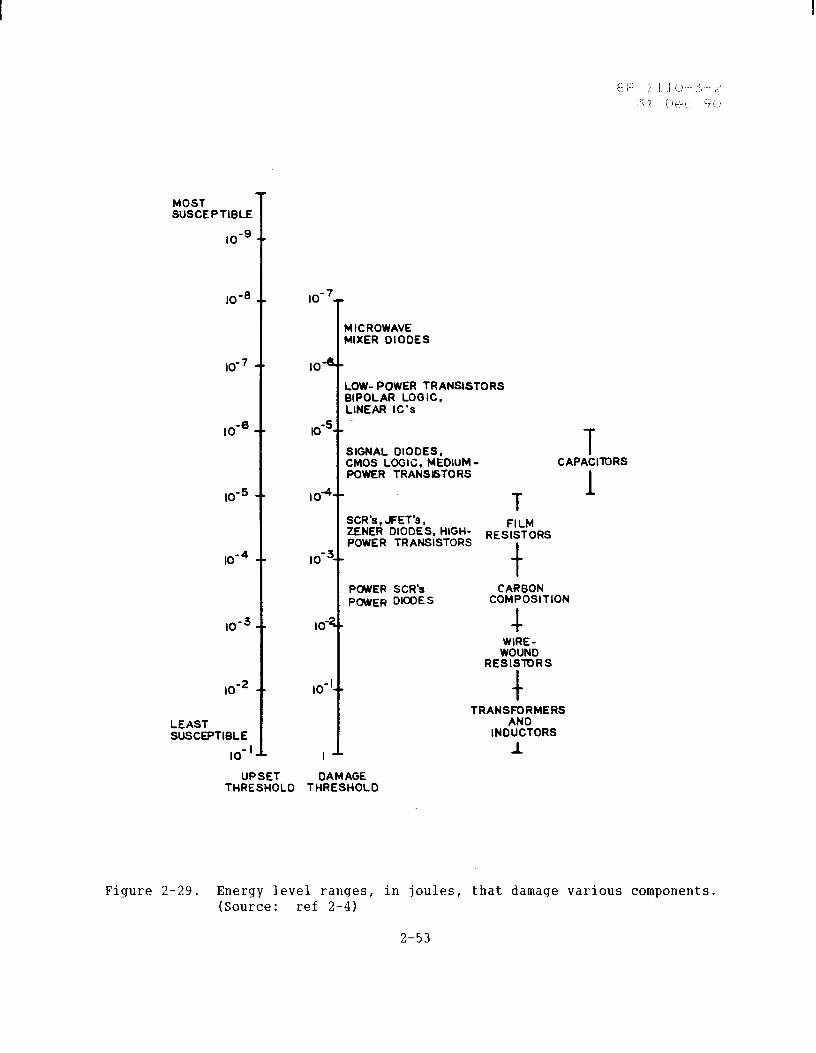
a. Equipment response. HEMP produces two distinct responses by equipment and system components: upset and damage. Upset is a nonpermanent change in system operation that is self-correcting or reversible by automatic or manual means. Damage is an unacceptable permanent change in one or more system parts. The spectrum of thresholds for some system components is shown in figure 2-29. The figure clearly shows that semiconductors are highly susceptible to HEMP and thus need protection.

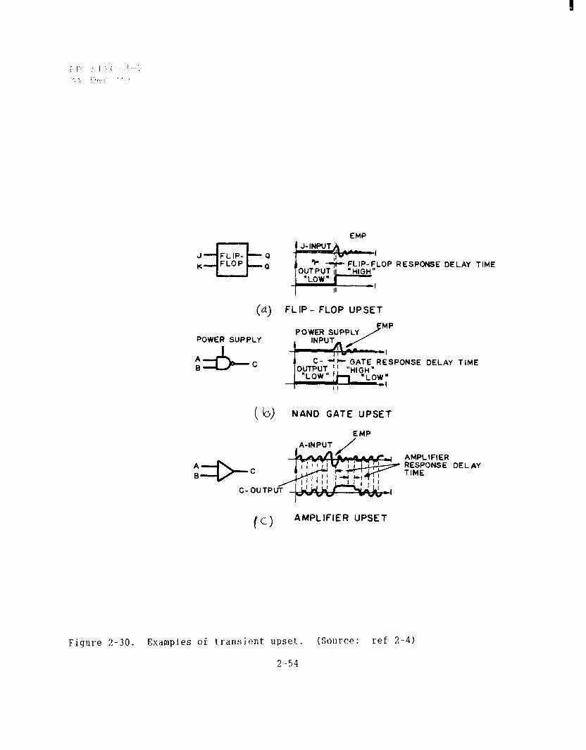
(1) Upset. Transient upset has a threshold about one order of magnitude below the damage thresholds. It occurs when an induced HEMP transient exceeds the operating signal level. It has a time scale that falls within the circuit’s time response. Figure 2-30 shows some examples of upset. Figure 2-30(a) shows a flip-flop changing state due to a HEMP transient on the trigger input. Figure 2-30(b) shows a NAND gate with a temporary change in its output logic level from a HEMP transient on the power supply line. Figure 2-30(c) shows an amplifier driven to saturation by a HEMP transient superimposed on its signal input.

(2) Damage.

(a) Semiconductors. Damage to semiconductors due to applied transients is typically some form of thermal-related failure and therefore is related to the total energy applied to the device. For discrete devices (transistors, diodes), the predominant failure mode appears to be localized melting across the junction. The melted regions form resistive paths across the junction which short out the junction or mask any other junction action (ref 2-7). Metallization burnout resulting in open circuits has also been identified as a failure mode in integrated circuits (ref 2-8). A convenient

2-17

approach for failure analysis is the concept of the power failure threshold (Pth) (ref 2-I). The power failure threshold is defined as--

‘th = At-b (eq 2-8)

where A is the damage constant based on the device material and geometry, and b is the time-dependence constant. The constants A and b can be determined empirically for every device of interest by the least-squares curve fit to experimental pulse test data. In general, it will be more convenient to use the Wunsch model (ref 2-7) for the power failure threshold with previously determined values of the Wunsch model damage constant for any analysis. This theoretical model has a time-dependence constant of b = l/2. Empirical data for a wide range of devices fits the model within the experimental data spread in the midrange of pulse widths, approximately 100 nanoseconds to 100 microseconds (ref 2-l). The Wunsch model theoretical equation is--

‘th = Kt-1’2 Kw/cm2 (eq 2-9)

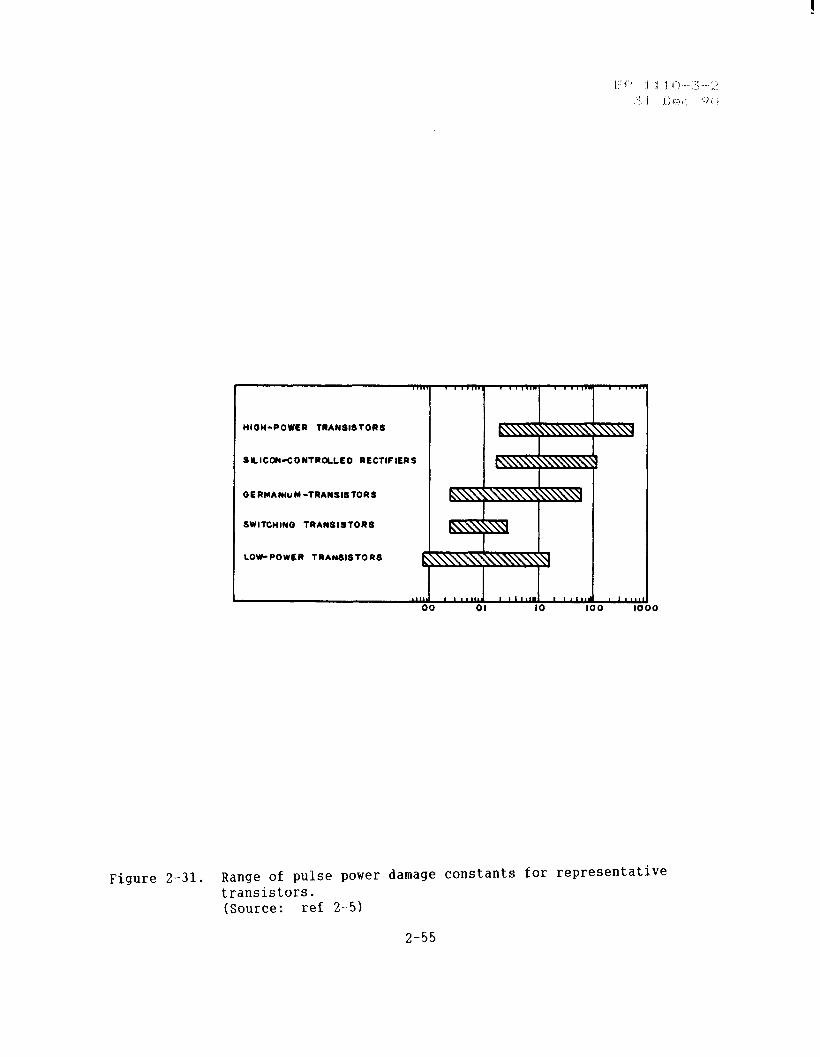
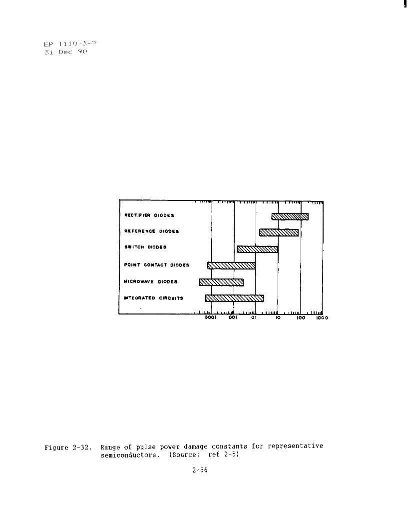
where t is the pulse width in microseconds and K is the Wunsch model damage constant in kW - (microsecondlI/2. K is expressed in these units since the numerical value of K is then equal to the power necessary for failure when a l-microsecond pulse is applied to the junction. Figures 2-31 and 2-32 show typical ranges for K for various semiconductors. Multiplication of this factor by te1j2 will yield the pulse power threshold.

(b) Passive elements. The passive elements most susceptible to damage from HEMP-induced currents are those with very low voltage or power ratings and precision components for which a small change is significant. Resistor failures due to high-level pulsed currents are caused by energy- induced thermal overstress and voltage breakdown. Resistor failure threshold can be calculated from the resistor’s parameters and the empirical relation given in reference 2-9. Exposure of capacitors to transient currents sets up a voltage across the capacitor that increases with time. For nonelectrolytic capacitors, this voltage keeps rising until the capacitor’s dielectric breakdown level is reached. That point is typically 10 times the d.c. voltage rating. For electrolytic capacitors, the voltage relationship holds until the zener level of the dielectric is reached. After that, damage can occur. The damage threshold for electrolytic capacitors in the positive direction is 3 to 10 times their d.c. voltage rating. For the negative direction it is one-half their positive failure voltage (ref 2-10). Transformer and coil damage due to HEMP-induced currents results from electric breakdown of the insulation. The pulse-breakdown voltage is typically 5500 volts for power supply transformers and 2750 volts for small signal transformers (ref 2-11).

b. Equipment sensitivity. Localizing responses of specific circuits or components within equipment or a system often is not possible for complex equipment. Therefore, when estimating system response, it is often more

2-18

realistic to deal with the thresholds at the equipment level instead of at the circuit or component level. Using the equipment thresholds approach usually requires that the applicable systems have had their thresholds analyzed or measured. Measured thresholds for some types of communications equipment are given in table 2-3.

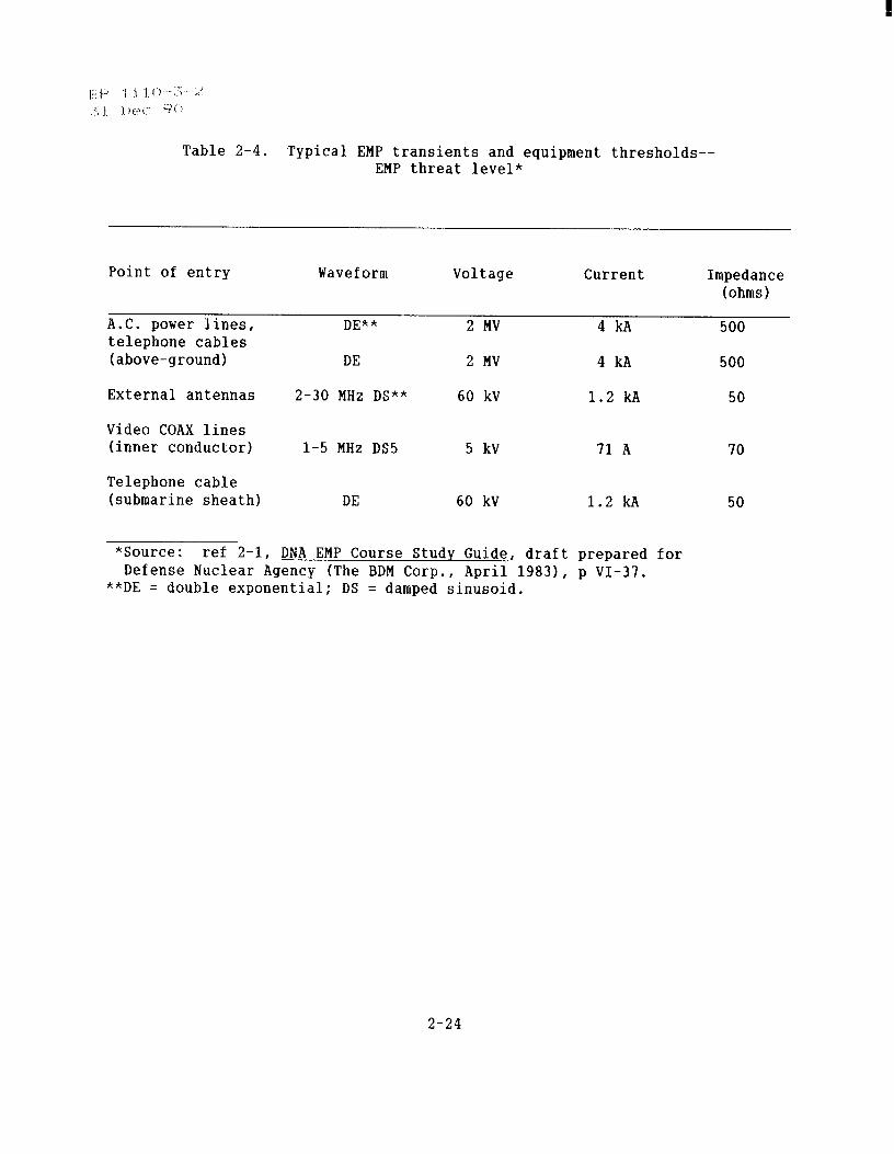
C. Typical damage and upset levels. Table 2-4 gives typical HEMP-induced transient levels as observed in tests and analyses at operational facilities. The largest voltage value is 2 megavolts and the largest current is 4 kiloamps. Much smaller values may also result. This is especially true for the inner conductor of the coaxial line because of the shielding protection provided by the outer conductor. The data in Table 2-4 were obtained with the equipment under test in a parallel plate EMP simulator. The simulator excitation approximated the 50-kilo- volt/meter double exponential waveform with risetime of 5 to 10 nanoseconds and e-fold of approximately 0.5 microseconds. A current probe was then used to measure the peak-to-peak current on a power supply lead. The current measured was typically a damped sinusoid with frequency dependent on equipment type and lead length.

2-6. Cited references.

2-l. DNA EMP Course Study Guide, draft prepared for Defense Nuclear Agency (The BDM Corporation, April 1983).

2-2. Ghose, Rabindra N., EMP Environment and System Hardness Design, Library of Congress Catalog Card Number 83-51062 (Don White Consultants, Inc., Gainesville, VA, 1984).

2-3. DOD-STD-2169, (U) High-Altitude Electromagnetic Pulse (HEMP) Environment (DOD, June 1985) (5).

2-4. Prototype HEMP Design Practice Handbook, prepared for Defense Communications Agency, Contract No. DCA 100-77-C-0040 (IRT Corporation, 31 May 1978).

2-5. EMP Awareness Course Notes, DNA 2772T (HQ, Defense Nuclear Agency, August 1971).

2-6. Lee, K. S. H., EMP Interaction: Principles, Techniques, and Reference Data, AFWL-TR-80-402, (Dikewood Industries, Albuquerque, NM, December 1980).

2-7. Wunsch, D. C., and R. R. Bell, “Determination of Threshold Failure Levels of Semiconductor Diodes and Transistors due to Pulse Voltages,” IEEE Transactions on Nuclear Science, NS-15, No. 6 (Institute of Electrical and Electronic Engineers, December 1968).

2-19

2-8. Jenkins, C. R., and D. L. Durgin, “EMP Susceptibility of Integrated Circuits,” IEEE Transactions on Nuclear Science NS-22, No. 6 (Institute of Electrical and Electronic Engineers, December 1975).

2-9. Tasca, D. M., D. C. Wunsch, and H. Domingos, “Device Degradation by High Amplitude Currents and Response Characteristics of Discrete Resistors, ” IEEE Transactions on Nuclear Science, NS-22, No. 6 (Institute of Electrical and Electronic Engineers, December 1975).

2-10. Tasca, D. M., H. B. O’Donnell, and S. J. Stokes III, Pulse Power Responses and Damaqe Characteristics of Capacitors, Final Report, Contract F29601-75-C-0130 (General Electric, December 1976).

2-11. Dunbar, W., and J. Lambert, “Power System Component EMP Malfunction/Damage Threshold,” paper presented at DNA EMP Seminar IIRI, Chicago, IL, 14-16 May 1974.

2-7. Uncited references.

DNA EMP Handbook, DNA 2114H-2, Vol 2 (Defense Nuclear Agency, November 1971).

Lee, K. S. H., T. K. Liu, and L. Morins, “EMP Response of Airdraft Antennas, ” IEEE Transactions on Antenna Properties, AP-26, No. 1 (Institute of Electrical and Electronic Engineers, January 1978).

EMP Design Guidelines for Naval Ship Systems, ITTR NSWC/WOL/TR-75- 193, Naval Surface Weapons Center, 22 August 1975.

EMP Engineering and Design Principles, Bell Laboratories, PEM-37 (Lawrence Livermore Laboratory, 1975).

MIL-STD-461C, Electromagnetic Emission and Susceptibility Requirements for the Control of Electromaqnetic Interference (DOD, 4 August 1986).

2-20

Table 2-l. Important features of EMP environments*

Type Features Systems impact

HEMP

Surface-burst

Source region

Radiated region

Air-burst

Source region

Radiated region

SGEMP

MHD-EMP

Large extent, high amplitude, broad frequency band, plane wave

Large amplitude, limited Important for systems which extent includes varying are hard to other nuclear conductivity, currents effects

Large amplitude varies inversely with distanc,e

Can supersede HEMP if vertical orientation or low freqs. important

Similar to surface-burst

Amplitude less than HEMP

Very high amplitude and fast rise time

Very low frequency, low amplitude, large extent

Most widely specified threat

See surface burst

Superseded by HEMP

Important for exoatmospheric systems

May affect long-land or submarine cables

*Source : ref 2-1, DNA EMP Course Study Guide, draft prepared for Defense Nuclear Agency (The BDM Corp., April 19831, p I-51.

2-21

Table 2-2. EMP waveform summary*

Type

Peak amplitude Timeframe

HEMP

Surface-burst

Source region

Radiated region

Air-burst

Source region

Radiated region

SGEMP 100 kV/m

MHD-EMP 30 V/km

50 kV/m Few nanosec to 200 nanosec

1 MV/m

10 kV/m

10 kV/m

Few nanosec to 1 microsec

1 microsec to 0.1 set

1 microsec to 100 microsec

Similar to surface- burst

300 V/m at 5 km, typical (highly dependent on HOB

10 nanosec to 5 microsec

Few nanosec to 100 nanosec

0.1 set to 100 set

*Source: ref 2-1, DNA EMP Course Study Guide, draft prepared for Defense Nuclear Agency (The BDM Corp., April 1983), p I-49.

2-22

Table 2-3. Response thresholds*

Equipment Lead**

Max. stress Upset level, Damage level, level,

p-p*** P-P P-P (A) (A) (A)

Primary frequency supply (PFS-2A) -24 V 0.4 --+ -9

A5 channel bank (solid state modem) -24 V 80

input --

gain --

Multiplex WELMX-1 (tube) WELMX-2 (solid-state) WEMMX-1 (tube) WEMMX-2 (solid-state)

130 v 0.07 -24 V 0.02 130 v 2 -24 V --

Wireline entrance link, 3A (amplifier) -24 Vl 1 35

100-A protection switch (switching unit)

+24 V 0.2 -- 0.9

TM-1 radio-27 V .- 25 25

L4 cable system Trigger A equalizer Protection switch

-24 V 8 -24 V 16

WE TD3 radio dc power input 50 WE TH3 radio dc power input 60 Farinon FM 2000 radio dc power input 208 Lenkurt 778A2 radio dc power input 35 Collins MW608D radio dc power input 50‘

--

150 75

--

60 --

--

--

240 --

150 150

75

1 60

2 50

110 110

--

*Source : ref 2-4, Prototype HEMP Design Practice Handbook, prepared for Defense Communications Agency (IRT Corp., Contract No. DCA 100-77-C-0040, May 1978).

**Point where induced current was measured. ***Induced peak-to-peak (damped sinusoid) on indicated lead.

+Data not measured.

2-23

,;i, I.:.’ ./ ., :, (:) ,.::, t-’

: i:; :, !, 1 (,i (1; ‘“i ( !

Table 2-4. Typical EMP transients and equipment thresholds-- EMP threat level*

Point of entry Waveform Voltage Current Impedance (ohms)

A.C. power lines, telephone cables (above-ground)

DE** 2 MV 4 kA 500

DE 2 MV 4 kA 500

External antennas 2-30 MHz DS** 60 kV 1.2 kA 50

Video COAX lines (inner conductor) l-5 MHz DS5 5 kV 71 A 70

Telephone cable (submarine sheath) DE 60 kV 1.2 kA 50

*Source : ref 2-1, DNA EMP Course Study Guide, draft prepared for Defense Nuclear Agency (The BDM Corp., April 19831, p VI-37.

**DE = double exponential; DS = damped sinusoid.

2-24

CHARGE SEPARATION

SECONDARY ELECTRONS COMPTON

A I R MOLECULE ELECTRON

- BURST

SCATTERED T RAY

THE COMPTON PROCESS PRODUCES CHARGE SEPARATION HIGHLY ENERGETIC FREE ELECTRONS

Figure 2-l. The Compton process. (Source : ref 2-l)

2-25

This page not used.

2-26

TANGENT RADIUS

SURFACE ZERO

REGION OF MAXIMUM PEAK ELECTRIC FIELD

Figure 2-3. Variations in high-altitude EMP peak electric field strength as a function of direction and distance from surface zero. (Source: ref 2-l)

2-27

FOURIER AMPLITUDE OF ELECTRIC FIELD

KV-S/M

cn F r

ELECTRIC FIELD ( KWM I

0

0

kb

b “ccnap~- 0000,~

MAGNETIC FIELD (A/M)

ELECTRIC FIELD ( KV/M 1

MAGNETIC FIELD (A/M)

/

I

IO”

EARLY-TIME INTERMEDIATE -TIME I LATE- TIME

PROMPT GAMMA SIGNAL

SCATTERED GAMMA SIGNAL

NEUTRON INELASTIC SIGNAl

MHD SIGNAL

TIME (S)

Figure 2-5. Qualitative time domain example of HEMP. (Source: ref 2-l)

2-29

I HIGH FREOUENCY (HEMP)

1

-3 IO I IO3 IO

8 lOa

FREOUENCY (Hz)

Figure 2-6. Qualitative frequency domain example of HEMP. (Source: ref 2-l)

2-30

i-’ j .,’ ./ / \ I /... :; .-‘,::

:!< ! ,...I, i ,:,.,>,.

SURFACE BURST EMP

* SOURCE REGION F IEL DS AND CURRENTS ARE SIGNIFICANT FOR HARDENED SYSTEMS

l SIGNIFICANT RADIATEIJ FIELDS EXTEND 0114 ‘10 MORE THAN IO Km

Figure 2-7. Surface-burst EMP showing source region and radiated region. (Source : ref 2-l)

2-31

DEPOSITION REGION BOUNDARY - ~

.VECTOR SUM OF ALL

RAOIAL ELECTRIC FIELD FROM CHARGE SEPARATION\

/ COMPTON CURRENTS

I RESULTS IN VERTICAL DIPOLE

\ /’ \ CURRENT LOOPS FORMED BY J-’ ‘AZIMUTHAL MAGNETIC FIELD 84 ELECTRON FLOW OUTWARD NEAR SURFACE CAUSED IN AIR AND RETURN THROUGH BY CURRENT LOOPS GROUND

Figure 2-8. Overview of surface-burst EMP. (Source : ref 2-l)

2-32

c! N 4. I t-2

I I I I 0 AMPLITUDE TYPICALLY LESS THAN HglP

OUTSIDE SOURCE REGION

l AMPLITUDE VARIES INVERSELY WITH RANGE OUTSIDE SOURCE REGION

0 NO STANDARD WAVEFORM

_ 0 SYSTEM IMPACT MAY SUPERSEDE HEMP DUE TO - HIGH LOW-FREQUENCY CONTENT (BELOW 100 kH$ -VERTICAL E-FIELD ORIENTATION

2 4 6 0 IO

R (km)

._

Y. + .._

y$ .‘- -. :-: j

: : .’ .: _.-

<;-;

.f ‘)..‘

L

/i:, j:-. 1, , ‘, < ‘j .:I; ,,:

,‘, 1 , !c.;,(’ I:.)!, ,

0

0

WEAPON GAMMAS

CHARGE SEPARAT FIELO (-Efr)

NO SIGNIFICANT FIELDS

SCATTER COMPTON ELECTRONS

‘ION PROOUCES RADIAL ELECTRIC

CURRENT LOOPS OR MAGNETIC

Figure 2-10. Air-burst EMP--source region.

2-34

+

+

+ ’ .

+ -

+

r ATMOSPHERIC DENSITY GRADIENT PRODUCES WEAK VERTICAL DIPOLE

\ \ ,;

1, RP

\ F \ \

-1

1

rDlA :IEL

c \

l ATMOSPHERIC DENSITY GRADIENT RESULTS IN ASYMMETRIC CHARGE DISTRISUTION

rTED l RESULTANT VERTICAL DIPOLE DIATES WEAK

.DS -VERTICAL ELECTIC FIELDS ( -AZIMUTHAL MAGNETIC FIELDS? ,J k

. WATER VAPOR DENSITY GRADIENT CONTRIBUTES TO ASYMMETRY AND RADIATION

. GEOMAGNETIC TURNING OF COMPTON ELECTRONS ADDS HEMP- LIKE COMPONENT

-. -

/;, c .’ ! i l/I .!( ,.:

.:, ‘! i,i!..ai, I :. 2, :

EO

INCIDENT HEMP APERATURE PENETRATION

DIRECT ENERGY INJECTION FROM INTENTIONAL AND ADVERTENT ANTENNAS

EXTERIOR REGION

SHIELDED ENCLOSURE

Figure 2-12. Three modes of penetration and coupling into shielded enclosures. (Source: ref 2-4)

2-36

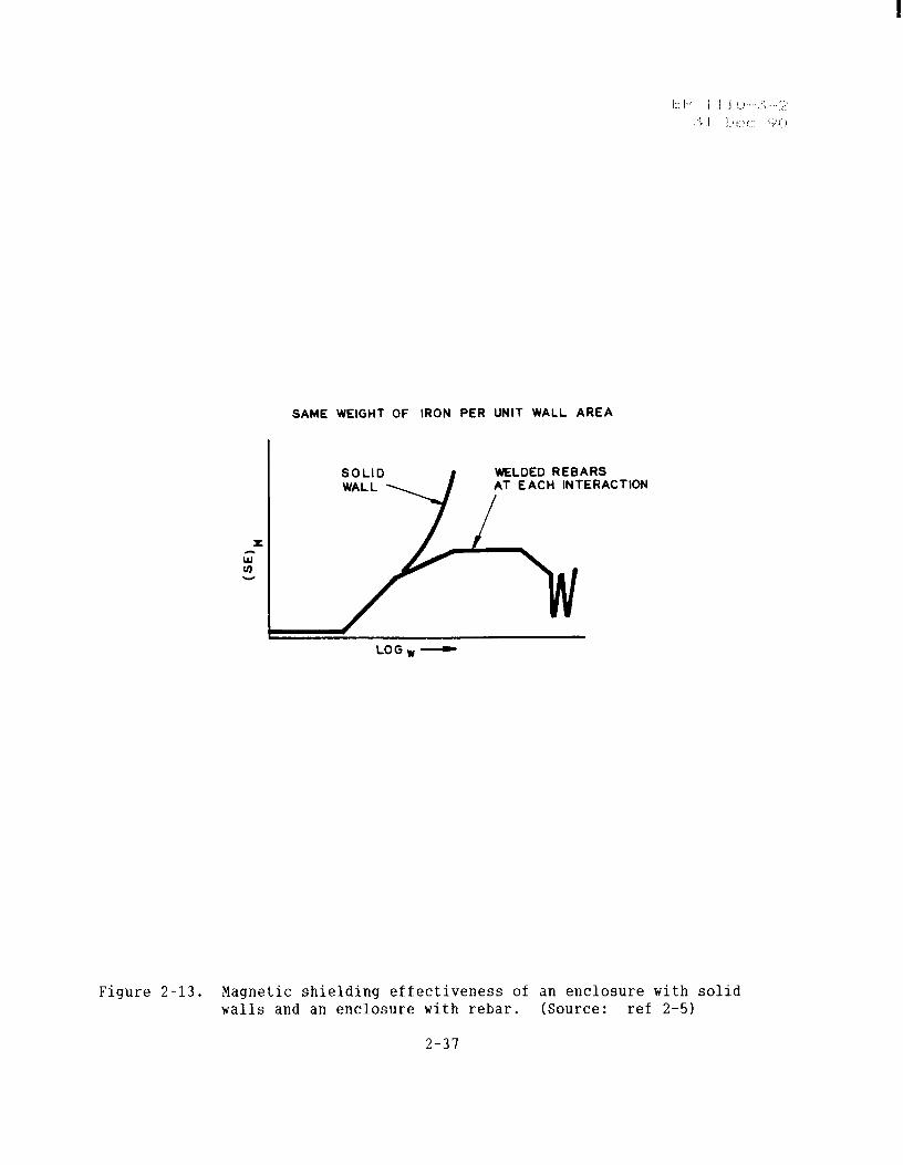
SAME WEIGHT OF IRON PER UNIT WALL AREA

WELDED REBARS

LOGw-

Figure 2-13. Magnetic shielding effectiveness of an enclosure with solid walls and an enclosure with rebar. (Source : ref 2-5)

2-37

IOE AL

HOLE RESONANCES

LOG w - HOLE OIAMETER APPROXIMATES WAVELENGTH

Figure 2-14. Magnetic shielding effectiveness of an ideal enclosure and an enclosure with openings. (Source: ref 2-5)

2-38

\ I \

‘YY .d -Ld d Y ”

7

v 99

COMMERCIAL POWER

WR a COCLANT FOR HEAT EXCHANGERS

Figure 2-15. Ground-based facilities--unintentional antennas. (Source : ref 2-l)

2-39

DOOR

BURIED CONDUIT

-FACILITY PENETRATIONS

Figure 2-16. EMP coupling to facility penetrations. (Source : ref 2-l)

2-40

EQUIP

MAGNETIC INDUCTION

738 - - -

EQUIPMENT

I VXE=-dB

dt f

t

LOOP OF AREA A

ELECTRIC INDUCTION

WENT

- A

Figure 2-17. Two mechanisms by which EMP couples to conductors. (Source: ref 2-l)

2-41

1 h

FOR LARGE RL:

FOR SMALL RL:

Voc : EW -INOUCED OPEN C I RCU I T VOLTAGE

VL : EMP - I NOUCED LOAD VOLTAGE

f w L

u RL CA T CA ; ANTENNA CAPACITANCE

RL : LOAD RESISTANCE

2, : INTRINSIC IMPEDANCE OF ANTENNA

VL:\bc’ -h ESlN0 (NEGLGIBLE FOR SMALL h)

VL l -hRLC,$$ SIN8

Figure 2-18. Equivalent circuit for a small electric dipole. (Source : ref 2-l)

2-42

EP 1110-3-11 31 Dee 90

FOR LARGE RL, VL’ VOy -A , P

F\. FOR SHALL y.VL - -A - B bl

y)c 1 EMP-INDUCED OPEN CIRCUIT VOLTAGE .

’ L : EHP-INDUCED LOAD VOLTAGE

LA I ANTENNA INDUCTANCE

R L : LOAD RESISTANCE

Figure 2- 19. Equivalent circuit for a mall loop (magnetic dipole). (Source: ref Z--l)

2-43

EQUIVALENT FAT MON 0 POLE

r GROUND PLANE

Figure 2-20. Modeling example--microwave tower and equivalent fat cylindrical monopole. (Source: ref 2-l)

2-44

AV = Is ZTAX

AV = VOLTAGE DROP ON CENTER CONDUCTOR OF CABLE OF LENGTH AX

IS = SHEATH CURRENT

ZT = TRANSFER IMPEDANCE PER UNIT LENGTH

AX = INCREMENTAL LENGTH

Figure 2-21. Shielded cables and transfer impedance. (Source : ref 2-l)

2-45

OVERHEAD LINE WITH LOADS

E

A H S

EQUIVALENT TRANSMISSION LINE FOR EMP COUPLING

Figure 2-22. Transmission line coupling. (Source : ref 2-l)

2-46

LINE LENGTH - M

Figure 2-23. Aerial conductors: effect of conductor length. (Source : ref 2-l)

2-47

a I

= 250 nsec = IO -2 mho/m

200

loo

0

0 0.5 1.0 I 5

TIME - J,(Sec

Figure 2-24. Buried conductors: effect of burial depth. (Source: ref 2-l)

2-48

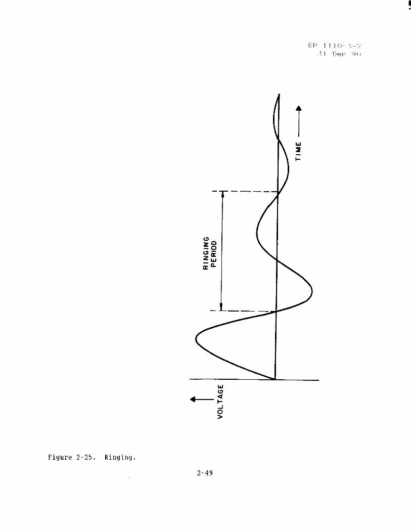
Figure 2-25. Ringing.

2-49

CABLE TRAY8 \

ANAL ANO POWER pUCT8

AC OlSTRlBUTlON PANEL

I

P, MAIN 0 DISTRIEI

/h=== UTlON//

“‘..vA

AND DIOITAL

/ 1 w :“pfu:%iA$T

.I I \ ROMEX CABLE OROUWD~CABLE TRAYS7 VOT OR SIMILAR -

OlOlTAL EOuiPt4E~t

AC ROWEX CABLE (MODEMS)

@ROUND ROD

Figure 2-26. Typical internal signal cable distribution diagram. (Source : ref 2-l)

2-50

DIRECT ILLUMINATION FOR A TYPICAL UNSHIELDED COMMUNICATIONS FACILITY

THAN ABSClssa

40-

20 -

2 4 6 0 IO 12 14 16

CURRENT COUPLED TO EOUPMENT LEADS

Figure 2-27. Intrasite cables. (Source: ref 2-l)

2-51

I EMP FLLbS l TENS OF w/m I

. TENS OF KILOAMPS CONDUCTORS . HUNDREDS OF KILOVOLTS

. TENS OF AMPS l HUNDREDS OF VOLTS

DEORADATION

Figure 2-28. EMP system interaction. (Source : ref 2-l)

2-52

i::. 1.‘. / ‘, ,/ , j .I /..... ,..a

,::, ‘1 (!(L( ‘.,, ,’ .,

MOST SUSCEPTlBLE

iO-g

10-a

10-7

lo-6

10-S

10-4

10-3

10-2

LEAST SUSCEPTl8LE

10-l

UPSET THRESHOLD

MICROWAVE MIXER DIODES

LOW- POWER TRANSISTORS BIPOLAR LOGIC, LINEAR IC’s

I SIGNAL DIODES, CMOS LOGIC. MEDIUM - POWER TRANSISTORS

T CAPACITORS

I

T ’ SCR’s, #ET’s, ZENER DIODES, HIGH- R&+;RS POWER TRANSISTORS

t

POWER SCR’s CARSON POWER DIODES COMPOSITION

m 4 WIRE- WOUND

RESISTORS

TRANSFORMERS AND

INOUCTORS

OAMAGE THRESHOLD

Figure 2-29. Energy level ranges, in joules, that damage various components. (Source : ref 2-4)

2-53

EMP

LOP RESPONSE DELAY TIME

(“1 FLIP - FLOP UPSET

POWER SUPPLY

;t&rT jgk”IpoNsE OELAY TIME

( Q i NAND GATE UPSET

EMP

A-INPUT /

AMPLIFIER RESPONSE DELAY TIME

C-OUTP

4”) AMPLIFIER UPSET

Figure 2--30. Examples oi transient Upset. (Source : ref 2-4)

2--54

;.:: ,::.. / / ‘, < .! ,:; ‘;I

::. i , ),:;q- ‘.:!; 1: ,,

HIOH-POWER TRANSISTORS

SiLlCOR-CONtROLLED RECTIFIERS

OERMANIUY-TRANSISTORS

SWITCHINO TRANSI8TORS

LOW-POWER TRAN8lSTORS

I 00 01 IO 100 1000

Figure 2-31. Range of pulse power damage constants for representative transistors. (Source: ref 2-5)

2-55

RECTIFIER OIOOES

RtFERENCL OIOOES

SW ITCN DIODES

POINT CONTACT OIOOCS

YlcROWAVE OlOOES

INTEORATED CIRCUITS

L loo la

Figure 2-32. Range of pulse power damage constants for representative semiconductors. (Source : ref 2-5)

2-56