Chapter 2 Computer Modeling of Transport Layer Effects

Chapter 2Computer Modeling of TransportLayer Effects

André Richter

Abstract This chapter introduces the reader into optical signal representationsand the major physical layer effects causing system degradations in the WDMtransport layer. Suitable modeling approaches are presented, and typical simula-tion results are demonstrated. Finally, the chapter focuses on performancedegrading effects due to fiber propagation, optical amplification, and signalgeneration.

2.1 The Value of System-Level Simulation

System-level simulations are now routinely used to theoretically evaluate theperformance of transmission systems based on the parameters of existing opticalequipment, and to define performance requirements for new equipment to ensurerobust operation for all required application scenarios. In a sense, system simu-lation is used as a virtual prototyping tool that reduces cost by shortening thesystem construction cycle. Furthermore, simulations prove valuable for investi-gating possible upgrade scenarios, understanding the nature and sources forsystem-limiting effects, determining the full effect of component limitations, anddeveloping new technological approaches. The most critical part in designingaccurate and reliable system simulation scenarios is selection of the rightparameters and accurate transport effect models.

A. Richter (&)VPIphotonics Division, VPIsystemsBerlin, Germanye-mail: [email protected]

N. (Neo) Antoniades et al. (eds.), WDM Systems and Networks, Optical Networks,DOI: 10.1007/978-1-4614-1093-5_2, � Springer Science+Business Media, LLC 2012

13

2.2 Simulation Domains and Signal Representations

For computer simulation to be effective, optical signals need to be represented intothe computer. Optical signal representations with different degrees of abstractionare important in providing flexibility for modeling various aspects of photonicnetworks. Since the initial publications of the fundamental concept as in Loweryet al. [1], many improvements have been introduced supporting the modelingrequirements of the ever-evolving advances in optical technologies and networkarchitectures [2].

Time-domain simulations that propagate individual time samples on an iteration-by-iteration basis between modeling blocks have been used to investigate, forinstance, the properties of integrated photonic circuits, high-speed transmitters, andreceivers, where the analysis of bidirectional interactions in the picoseconds rangeare of key importance [3]. For optical systems and networking applications mixed-domain simulations (i.e. including both, the time- and frequency-domains) are moresuitable where arrays of signal samples are passed between modeling blocks.Applications are mainly unidirectional propagation scenarios and bidirectionalscenarios where time delays are longer than the array duration (e.g., opticalswitching scenarios in bidirectional ring networks), or where bidirectional inter-actions can be averaged in time (e.g., bidirectional Raman pumping of optical fiber).

The simulation efficiency of mixed-domain simulations can be controlled byrepresenting optical signals either by their complex, polarization-dependent sam-pled waveform (time-dynamic or spectral representation), or by time-averagedparameters only. Depending on the modeling scope of interest, the time-dynamicrepresentation can be applied to a single frequency band (SFB), or to multiple(non-overlapping) frequency bands (MFBs) for which the appropriate propagationequations describe the evolution of individual frequency bands, while interactingterms are approximated using frequency decomposition (FD) techniques.

Although waveform-dependent propagation effects are ignored when using aparameterized representation of optical signals, this approach provides significantsimulation speed-up while keeping sufficient modeling accuracy when investi-gating, for instance, the impact of ‘far-away’ WDM channels or optical pumps.Parameterized Signals (PS) can also be used to track important properties along thetransmission path such as power, principal states of polarization (PSP), as well asaccumulated amounts of noise, chromatic dispersion (CD), self-phase modulation(SPM), differential group delay (DGD), and thus easily assess signal characteris-tics over topology and frequency. Additive noise that is generated by lumped ordistributed optical amplifiers can be tracked separately from the optical signal,disregarding nonlinear interaction effects between noise and signal, or accountingfor them at the receiver using deterministic system performance estimation algo-rithms. In that case, optical noise can be described by its wavelength-dependentpower spectral density (PSD), which could be step-wise approximated by so-calledNoise Bins (NBs) of constant PSD. Further on, the parameterized representation isuseful for keeping parasitic terms resulting from optical amplification, crosstalk,

14 A. Richter

and scattering processes (collectively called Distortions) separate from theoptical signal, and thus, allowing the investigation of their impact on the signalquality.

2.3 Device Modeling

Different levels of abstraction in device modeling help to address the tradeoffsbetween the model complexity, simulation accuracy and computation speed [4]thus allowing the researcher to choose the required depth of detail. Typically,detailed models require in-depth parameters, whereas behavioral models operateon measured characteristics, or information from data sheets. At one extreme,detailed physical models represent components based on material and structuralparameters. These parameters may be difficult to obtain, being proprietary,or difficult to derive from external measurements of a packaged device. Detailedphysical models may require intensive computation, but can be used to design newdevices and predict their performance. Black-box models are based on the physicsof the device, but can be described in terms of behavioral parameters (instead ofin-depth parameters), which can be directly derived from external measurements.Linear devices (such as filters) or well-specified devices (such as transmitters witha digital input) can be represented by their measured performance alone. Althoughnovel devices cannot be designed directly using these models, the system per-formance of a module is easily and accurately assessed using these methods. Datasheets often provide characteristics as a series of parameters fitted to measure-ments (such as rise-time, spectral width). Although such data are often gatheredusing long-term measurements, their wide availability makes it useful for systems-level simulation. Attention should be given so that long-term averages do notmisrepresent the worst case.

2.4 Fiber Propagation

Transmission effects influencing signal propagation over single-mode optical fibercan be grouped into several general categories arising from the fiber propertiesitself. There are first optical power loss effects, which are either regarded as beingequally distributed along the fiber distance (e.g., power attenuation) or occur atisolated points along the fiber due to discrete events such as splices and fiber ends.Further on, the velocity of light traveling through the fiber depends on thewavelength, which results into dispersive effects of information-carrying opticalsignals. The so-called group velocity dispersion (or CD) is a linear propagationeffect, which could theoretically be reversed after fiber propagation by means thatare independent of the transmitted signal, for example, using components withopposite dispersion such as using dispersion compensating fiber (DCF) or fiber

2 Computer Modeling of Transport Layer Effects 15

Bragg gratings (FBG). Additionally, power loss and dispersive propagationeffects might be dependent on the local polarization state in time and frequencydue to manufacturing imperfections, stress or other effects changing the prop-erties of the perfectly circular optical single-mode fiber. Important effectsare polarization mode dispersion (PMD) and polarization-dependent loss/gain(PDL/PDG).

In addition to the above-mentioned linear effects linear scattering processessuch as Rayleigh scattering, spontaneous Raman- and Brillouin- scattering arealso important to consider. Rayleigh scattering can be understood as distributedreflection of the light wave on microscopic in-homogeneities of the fiber med-ium. This effect significantly contributes to the fiber loss. Furthermore, doubleRayleigh scattering leads to a reflected lightwave propagating in the samedirection as the originating signal and therefore interferes with it. While thereflection strength is typically small, the effect may become significant in highamplifying media (for instance Raman amplifiers with high pump power).Spontaneous Brillouin and Raman scattering effects are caused by the scatteringof the lightwave on thermally induced acoustic waves or molecular oscillationsof the fiber medium (also referred to as acoustic and optical phonons, respec-tively). The importance of these effects results from the fact that the spontane-ously scattered signal becomes a seed for further amplification by the muchstronger nonlinear (stimulated) scattering effects, which are considered below.

Besides polarization-independent or dependent linear effects, signal trans-mission over optical fiber may suffer from effects, which result from the non-linear interactions of the fiber material and the light traveling through it.Nonlinear propagation effects can generally be categorized as effects involvinginstantaneous or almost instantaneous electronic contributions—the optical Kerreffect and its various manifestations as SPM, cross-phase modulation (XPM), andfour-wave mixing (FWM) as well as nonlinear effects with a noticeable timeresponse: stimulated Brillouin and Raman scattering (SBS and SRS) respectively.Depending on the response time the spectral bandwidth of these nonlinear effectsvaries from almost unlimited (in telecommunications terms) for the Kerr effect,intermediate for the Raman effect (in the vicinity of 13 THz) and rather small forthe Brillouin effect (linewidth of about 100 MHz and a Stokes shift of about10 GHz).

Finally, it is important to note that the nonlinear propagation effects occur incoexistence to CD, polarization effects, and attenuation, and may produce complexdegradations or beneficial interactions (depending on the system parameters underinvestigation). For example, the FWM efficiency depends strongly on the CD ofthe fiber; SPM can support very stable pulse propagation in the presence of theright amount of CD; the impact of PMD can be reduced by nonlinear fiberinteractions; the polarization dependence of SRS may introduce PDG. Thus,accurate fiber modeling needs to include nonlinear and linear phenomena, so thatdetrimental and beneficial interactions between these characteristics are predictedcorrectly.

16 A. Richter

2.4.1 Linear Propagation Effects

2.4.1.1 Attenuation

Fiber attenuation is mainly caused by absorption and scattering processes. It deter-mines the resulting exponential decay of optical input power propagating through thefiber. Absorption arises from impurities and atomic effects in the fiber glass. Scat-tering is mainly due to intrinsic refractive index variations with distance (Rayleighscattering) and imperfections of the cylindrical symmetry of the fiber. The usablebandwidth ranges from approximately 800 nm (increased Rayleigh scattering scaleswith k-4 [5, 6]) to approximately 1,620 nm (infrared absorption due to vibrationaltransitions). Older types of single-mode fiber show additionally an attenuation peakat approximately 1,400 nm due to the absorption of water molecules.

Typically being specified in logarithmic units as dB/km, sometimes it is usefulto work with attenuation values in linear units so:

a ¼ loge 10ð Þ10

� �adB=km � 0:23026adB=km ð2:1Þ

For single channel applications a can be assumed to be wavelength-indepen-dent. However, for applications covering a large spectral range, such as multi-bandWDM or Raman amplification, the spectral dependency of fiber attenuation shouldbe accounted for accurately in simulations.

The effective length Leff defines the equivalent fiber interaction length withrespect to constant power [7] so that:

Leff ¼Zz

0

e�az1 dz1 ¼1� e�az

að2:2Þ

In the above, Leff is an important quality measure when rescaling the signalevolution to account for attenuation and periodic amplification, and helpful whenperforming quick system performance estimations.

2.4.1.2 Chromatic Dispersion

The CD or group velocity dispersion (GVD) represents a fundamental linearpropagation limitation in optical fiber. It describes the effect that different spectralcomponents propagate with different group velocities. CD alone causes spreadingof chirp-less pulses along the fiber, although this statement is not true in general.For instance, in combination with nonlinear propagation effects other pulsepropagation characteristics are detectable. Note that CD is a collective effect ofmaterial and waveguide dispersion [6, 8]. Depending on the manufacturing processand the radial structure of the fiber, different fiber types with various CD profilescan be designed. In standard single-mode fibers (SSMF) the GVD is positive(i.e. shorter wavelengths propagate faster) for wavelengths longer than


approximately 1.3 lm and negative for shorter wavelengths. Thus, 1.3 lm is thepoint of zero GVD for SMFs. The fiber design allows shifting the point of zerodispersion and production of zero-dispersion fibers at 1.5 lm called dispersion-shifted fibers (DSF) or fibers with low positive or negative dispersion at thatwavelength called non-zero dispersion-shifter fibers (NZ-DSF), as well as fiberswith high negative dispersion values for dispersion compensation called DCF.

The impact of GVD on pulse propagation becomes clearer when expanding themodal propagation constant b(x) in a Taylor series around an arbitrary frequencyx0 as shown in Agrawal [9]:

b xð Þ ¼ n xð Þxc¼ b0 þ b1 x� x0ð Þ þ 1

2b2 x� x0ð Þ2þ 1

6b3 x� x0ð Þ3 ð2:3Þ

where n(x) is the effective refractive index of the fiber, c is the speed of lightin a vacuum, and bk ¼ ok=o xkbðxÞ at x ¼ x0 for k ¼ 0; 1; 2; 3 ði:e: partialderivative of bðxÞ with respect to x evaluated at x0Þ

In the above:

• b0 accounts for a frequency-independent phase offset during propagation cor-responding to the propagation constant at a certain reference frequency.

• b1 defines the inverse of the group velocity vg determining the speed of energypropagated through the fiber.

• b2 defines the GVD and describes the frequency dependence of the inverse of vg.It is responsible for the broadening of an initially chirp-less pulse due to the factthat its Fourier components propagate with different group velocities. This alsoleads to pulse chirp when the leading and trailing edges of the pulse contain lightwith different frequencies. Equivalently, it defines the different propagationspeeds of pulses in frequency-separated channels (such as in WDM systems).

• b3 is known as the slope of the GVD or second order GVD. This term accounts forthe frequency dependence of the GVD and therefore for the different broadeningproperties of signals or signal portions propagating at different frequencies. Thisterm is critical for wideband transmission systems, for systems operating in fre-quency regions where b2 is close to zero as well as systems utilizing DCFs tocompensate dispersion for multiple WDM channels simultaneously.

In general, it is of more interest to determine the dependence of the inverse ofthe group velocity vg on wavelength rather than on frequency. This dependence isdescribed by the dispersion parameter D and its slope with respect to wavelength,S. The following relationships inter-relate the above parameters:

D ¼ ddk

1vg¼ � 2pc

k2 b2 ð2:4Þ

S ¼ dD

dk¼ ð2pcÞ2

k3

1kb3 þ

1pc

b2

� �ð2:5Þ

18 A. Richter

b2 ¼d

dx1vg¼ � k2

2pcD ð2:6Þ

b3 ¼db2

dx¼ k3

ð2pcÞ2kSþ 2Dð Þ ð2:7Þ

D is typically measured in ps/nm-km and can be interpreted as describing thebroadening DT of a pulse with bandwidth Dk after propagation over a distance z, orequivalently, the time offset DT of two pulses after distance z that are separated inthe spectral domain by Dk.

DT is given below as:

DT � DkdT

dk¼ Dkz

ddk

1vg¼ DkzD ð2:8Þ

From the above, the walk-off length Lw can be defined as the distance it takesfor one pulse with duration T0 traveling at frequency x1 to overtake another pulsetraveling at frequency x2 and is thus given by:

LW ¼T0

b1 x2ð Þ � b1 x1ð Þj j �T0

DkDj j ð2:9Þ

The dispersion length LD characterizes the distance over which dispersiveeffects become important in the absence of other effects. Specifically, it defines thedistance over which a chirp-free Gaussian pulse broadens by a factor of

ffiffiffi2p

due toGVD and is given by:

LD ¼T2

0

b2j j¼ 2pc

k2

T20

Dj j ð2:10Þ

However, LD can also be applied as an approximation to determine the rele-vance of CD effects on other intensity modulated pulses. Since LD is inverselyproportional to the square of the signal bandwidth, as an example, the CDrequirement increases by a factor of 16 when increasing the signal bitrate from 10to 40 Gbit/s using the same modulation format and filter bandwidths that areproportional to the signal rate. In consequence, CD limits uncompensated 40Gbit/s NRZ transmission over SSMF to approximately 4 km and over NZ-DSF toapproximately 20 km. Additional dispersion variations due to changes in tem-perature along the link accumulate fluctuations as shown in Kato et al. [10] thathave to be compensated adaptively, especially in long-haul applications.

So it would be natural to think that low- or zero-dispersion fibers are theoptimum choice for WDM systems design. However, instead of using DSFs withvery small local GVD values, it is more appropriate to use transmission fibers withlarger local dispersion values (e.g., SSMF or NZ-DSF) and place DCFs at regulardistances along the link compensating for all or part of the accumulated CD theoptical signal experienced up to that point. If optical fiber were a purely linear


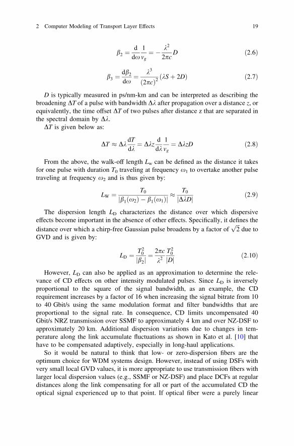
transmission medium it would not matter at which point along the link CD iscompensated. However, as will be described in the following section, fiberpropagation is slightly dependent on the intensity of the light traveling through it,thus resulting in nonlinear propagation effects. In modern WDM transmissionsystems with channel symbol rates of 10 Gbit/s and beyond, dispersion manage-ment taking care of the careful adjustment of local CD values (not too small) andmaximum accumulated CD before dispersion compensation (not too large) helpsto control these nonlinear fiber impairments (Fig. 2.1).

2.4.2 Nonlinear Propagation Effects

2.4.2.1 Kerr Effect

The Kerr effect denotes the phenomenon in which the refractive index of an optical

fiber n(x, t) is slightly dependent on the intensity of the optical signal IðtÞ ¼ EðtÞj j2,with E(t) being the electric field, passing through the fiber. As a result:

n x; tð Þ ¼ n0 xð Þ þ n2I tð Þ ð2:11Þ

where n0 is the linear refractive index and n2 is the nonlinear refractive index ofthe fiber.

When the electric field intensity of the transmitted signal bit stream varies intime it induces an intensity-dependent modulation of the refractive index, andhence, modulation of the phase of the transmitted signal. Compared to othernonlinear media, n2 is very small (typically on the order of 10-20 [m2/W]).However, even this weak fiber nonlinearity becomes fairly relevant for signalpropagation as field intensities of several mWs are focused in a small fiber core(in the order of several tens of lm2) over interaction lengths of tens to hundreds ofkilometers. As a result, effects such as nonlinear interaction between signal pulsesmight accumulate during transmission and become of system limiting importance.

In conclusion, the Kerr nonlinearity results in several intensity-dependentpropagation effects, with the most important ones being SPM, XPM, and FWM.

Fig. 2.1 Dispersionmanagement for a long-haultransmission experimentwhere dispersioncompensation is placed atregular intervals along thefiber as described inLiu et al. [11]

20 A. Richter

Self- and Cross-Phase Modulation

SPM and XPM occur when a temporal variation of the optical signal intensityinduces a temporal phase shift on the originating signal (SPM) or on otherco-propagating signals at different wavelengths (XPM).

For example, in the case where several optical signals at different wavelengthseach with intensity I(t) and initial phase u0 are launched into a fiber, the phasemodulation of the signal corresponding to channel m depends on the local powerdistribution of all other channels as follows:

um t; zð Þ � u0;m ¼ ulin;m þ uSPM;m þ uXPM;m

¼ 2pk

n0;mzþ 2pk

n2zImðtÞ þ4pk

n2zXk 6¼m

IkðtÞ ð2:12Þ

where um(t, z) is the phase modulation of channel m, u0, m is the initial phase ofchannel m, n0, m is the linear refractive index of channel m, n2 is the nonlinearrefractive index, and k is an index denoting the neighboring WDM channels ofchannel m.

Furthermore:

• ulin, m corresponds to the accumulated linear phase shift due to transmission.• uSPM, m corresponds to the accumulated nonlinear phase shift due to SPM in

channel m. The SPM-induced phase shift is proportional to the local signalintensity. It induces chirp (time-varying frequency shift) and spectral broaden-ing, so as an example, pulses behave differently in the presence of GVD andoptical filtering.

• uXPM, m corresponds to the accumulated nonlinear phase shift due to XPM inchannel m describing the phase modulation that is induced by intensity fluctu-ations in neighboring WDM channels. XPM introduces additional nonlinearphase shifts that interact with the local dispersion as well.

It must be noted that XPM occurs only over distances where optical intensitiesat different frequency components co-propagate, e.g. pulses propagating in dif-ferent WDM channels are overlapping. In general, the XPM effect reduces withincreased CD as pulses at different frequencies propagate faster through eachother, e.g. Lw (as defined in Sect. 2.4.1.2) becomes smaller. For the same reason,XPM scales inversely with the channel spacing. Lw is also called the collisionlength Lc as it accounts for the distance where two pulses at different frequenciescollide (and thus, interact nonlinearly due to XPM) during propagation.

Four-Wave Mixing

Parametric interactions between optical field intensities at different frequenciesmight induce the generation of inter-modulation products at new frequencieswhen propagating optical signals over wide spectral ranges through the fiber.


This nonlinear effect is called FWM. FWM can occur between channels in WDMsystems, between optical noise and channels, and between the tones within onechannel. More generally noted, FWM occurs for instance when two photons atfrequencies x1 and x2 are absorbed to produce two other photons at frequenciesx3 and x4 satisfying the relation below:

x1 þ x2 ¼ x3 þ x4 ð2:13Þ

It could also be understood as mixing of three waves producing a fourth oneaccording to the electrical field equations below:

Eklm ¼EkElE�m

¼ Ekj j Elj j Emj jej xkþxl�xmð Þte�j b xkð Þþb x1ð Þ�b xmð Þ½ �z ð2:14Þ

where Ei is the electric field of the wave propagating at frequency xi, b(xi) is themodal propagation constant at xi, and xklm = xk ? xl-xm is the carrier fre-quency of Eklm. The energy of Eklm is given as the superposition of mixingproducts of any three waves for which xklm = xk ? xl-xm holds (with thedegenerate case for xk = xl). Note that the propagation constant is frequency-dependent, so efficient interactions only occur if contributions to Eklm given atdifferent times add up over distance, e.g., the phase mismatch Db between theinter-modulating fields tends to go to zero (phase matching condition):

Db! 0; Db xð Þ ¼ b xkð Þ þ b xlð Þ � b xmð Þ � b xklmð Þ ð2:15Þ

The power of the newly created wave is proportional to the power of the threeinteracting waves assuming no pump depletion due to FWM occurs [12] resultingin:

Iklm zð Þ ¼ Eklm zð Þj j2¼ gc2klm Ek zð Þj j2 El zð Þj j2 Em zð Þj j2e�azL2

eff ð2:16Þ

where cklm is the nonlinear index of the fiber at xklm, a is the fiber attenuation, z isthe propagation distance, Leff is the effective length, and g is the so-called FWMefficiency given by:

g ¼ a2

a2 þ Db1þ 4e�az sin2ðDbz=2Þ

1� e�azð Þ2ð2:17Þ

FWM between the WDM channels scales inversely with channel spacing incase of non-zero GVD. Increasing the local dispersion results in an increased walk-off of the Fourier components and thus, it results in phase mismatch after shorterpropagation distances, which leads to an even steeper decrease of the FWM effi-ciency with channel separation.

Fig. 2.2 presents the results of a case study where four 10 Gbit/s NRZ signalsare propagated over 50 km of DSF and NZ-DSF fiber segments, respectively.Figure 2.2a shows the spectrum after transmission over 10 km of DSF, whileFig. 2.2b shows the corresponding spectrum after transmission over 10 km of

22 A. Richter

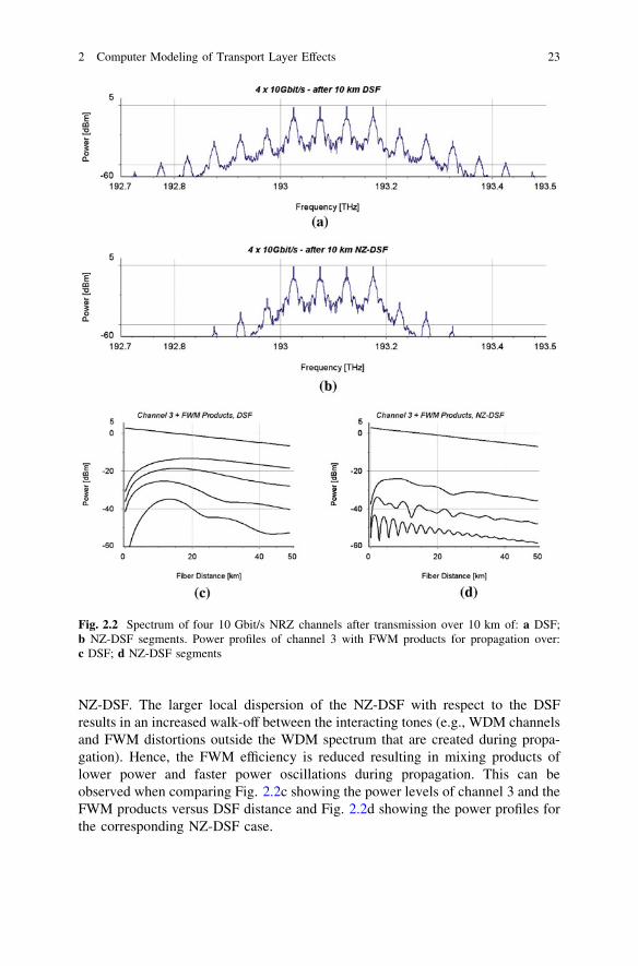
NZ-DSF. The larger local dispersion of the NZ-DSF with respect to the DSFresults in an increased walk-off between the interacting tones (e.g., WDM channelsand FWM distortions outside the WDM spectrum that are created during propa-gation). Hence, the FWM efficiency is reduced resulting in mixing products oflower power and faster power oscillations during propagation. This can beobserved when comparing Fig. 2.2c showing the power levels of channel 3 and theFWM products versus DSF distance and Fig. 2.2d showing the power profiles forthe corresponding NZ-DSF case.

Fig. 2.2 Spectrum of four 10 Gbit/s NRZ channels after transmission over 10 km of: a DSF;b NZ-DSF segments. Power profiles of channel 3 with FWM products for propagation over:c DSF; d NZ-DSF segments


The number of generated FWM components that are created when signalsat N wavelengths mix together grows with N2(N-1)/2. Using a sampled signalrepresentation, all important components that fall into the simulation band-width are automatically included when solving the fiber propagation equations(see Sect. 2.4.4.1). Note that the simulation bandwidth should be chosen wideenough in order to avoid misleading results due to aliasing effects of the generatedFWM components [13].

When accounting for FWM distortions using parametric modeling, the numberof calculated FWM components shall be limited to avoid excessive numericaleffort by considering only FWM distortions that would reach a certain powerthreshold, and thus, are important to be accounted for in system performanceanalysis.

Kerr Nonlinearities and CD

Similar to the dispersion length LD, a scale length for Kerr nonlinearities in opticalfiber could be defined: the nonlinear length LNL is given as the distance over whichthe phase of a pulse with intensity I changes by one rad due to the Kerr nonlin-earity in a fiber with a nonlinear coefficient c

LNL ¼1

cI2ð2:18Þ

LNL denotes the distance where nonlinear effects become important (in theabsence of other effects), also called nonlinear scale length. The ratio between LD

and LNL describes the dominating behavior for signal evolution in optical fiber. ForLD \ LNL linear effects dominate the signal propagation. In these quasi-linearsystems pulse powers change rapidly in time due to dispersion-induced pulsespreading and compression over LNL, and thus, the impact of nonlinear propaga-tion effects is averaged [14]. Those nonlinear pulse-to-pulse interactions can bebest described by time-equivalent terms of FWM and XPM, namely intra-channelfour-wave mixing (I-FWM) and intra-channel cross-phase modulation (I-XPM) asdescribed in Essiambre et al. [15], Mamyshev and Mamyshev [16]. Typically,I-FWM induces pulse echoes while I-XPM induces timing jitter. Pulse-to-pulseinteractions in quasi-linear systems become important for bitrates of 40 Gbit/s andhigher. With a careful selection of launch power, pre-chirp as well as the dis-persion map, degradations due to I-XPM and I-FWM can be drastically reduced(see for instance [17–19]).

Of special interest is also the case when LD * LNL. In these nonlinearity-supporting systems cancelation of dispersive and nonlinear effects can be observedfor carefully chosen system settings such as in soliton or dispersion-managedsoliton (DMS) systems. Choosing system parameters such as pulse width, sepa-ration, power, as well as dispersion map and amplifier position and separationcarefully, pulse chirp introduced by CD and SPM may combine and be used

24 A. Richter

advantageously for stabilizing pulse propagation over very long distances.However, XPM introduces timing jitter, which in addition to timing jitter inducedby added optical noise along the link is one of the ultimate limitations for suchsystems (see for instance [20]).

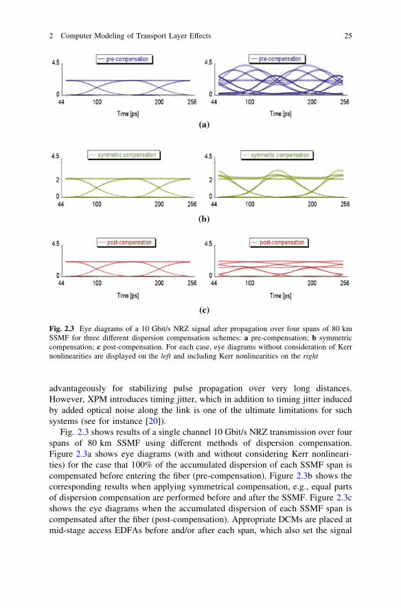
Fig. 2.3 shows results of a single channel 10 Gbit/s NRZ transmission over fourspans of 80 km SSMF using different methods of dispersion compensation.Figure 2.3a shows eye diagrams (with and without considering Kerr nonlineari-ties) for the case that 100% of the accumulated dispersion of each SSMF span iscompensated before entering the fiber (pre-compensation). Figure 2.3b shows thecorresponding results when applying symmetrical compensation, e.g., equal partsof dispersion compensation are performed before and after the SSMF. Figure 2.3cshows the eye diagrams when the accumulated dispersion of each SSMF span iscompensated after the fiber (post-compensation). Appropriate DCMs are placed atmid-stage access EDFAs before and/or after each span, which also set the signal

Fig. 2.3 Eye diagrams of a 10 Gbit/s NRZ signal after propagation over four spans of 80 kmSSMF for three different dispersion compensation schemes: a pre-compensation; b symmetriccompensation; c post-compensation. For each case, eye diagrams without consideration of Kerrnonlinearities are displayed on the left and including Kerr nonlinearities on the right


power into the transmission fiber at 10 dBm. Admittedly this value is rather large,though, it is chosen here in order to demonstrate the importance of consideringKerr nonlinearities when designing for an optimum dispersion map and amplifierplacement.

2.4.2.2 Scattering Effects

Stimulated Raman Scattering

Stimulated Raman scattering (SRS) is one of the most important scattering effects inoptical fiber. It denotes the inelastic process in which light is scattered by materialscattering centers, which causes vibrational excitation of molecules. As a result,energy is lost to the material with the effect that lower energy photons are createdfrom higher energy photons. Effectively, this means that signals at shorter wave-lengths are attenuated and signals at longer wavelength are amplified. SRS has animportant application for WDM systems, as relatively high distributed amplifica-tions may be achieved over the length of the transmission fiber. However, it may alsoinduce the Raman-induced tilt of WDM channel powers when the shorter wave-length channels become attenuated at the expense of longer wavelength channels.

Raman scattering is present at all optical frequencies, e.g., Raman amplificationcan be achieved at any wavelength (if an appropriate pump is available). Theamplification range using a single pump wavelength is broadband (about 6 THz at1.5 lm) but also strongly shaped. Raman amplifiers providing flat gain over largebandwidths require multiple pumps at different wavelengths [21] and a carefuladjustment of the individual pump powers [22, 23].

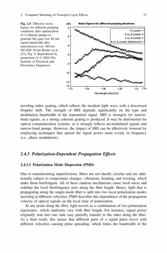
Besides stimulated Raman scattering, spontaneous Raman scattering occurs inthe fiber as well producing broadband optical noise that is strongly wavelength-and temperature-dependent. Additionally, double Rayleigh scattering may producesignificant amounts of additional noise. The pumping conditions (number andpower of co- and counter-propagating pumps) play an important role on the noisecharacteristics, as shown clearly in Figure 2.4.

Compared with EDFAs compensating fiber loss at the ends of links, Ramanamplification is low noise due to its distributed nature. Hence, Raman amplifica-tion allows lower launched powers while maintaining the OSNR, which reducesother nonlinear effects in the fiber.

Stimulated Brillouin Scattering

Stimulated Brillouin scattering (SBS) occurs when forward- and backward-propagating lightwaves induce an acoustic wave due to electrostriction with afrequency that equals the frequency difference of the optical waves, and apropagation constant that equals the sum of the propagation constants of theoptical waves (phase matching). In other words, the acoustic wave forms a

26 A. Richter

traveling index grating, which reflects the incident light wave with a downwardDoppler shift. The strength of SBS depends significantly on the type andmodulation bandwidth of the transmitted signal. SBS is strongest for narrow-band signals, as a strong coherent grating is produced. It may be detrimental foroptical communication systems, as it strongly reflects un-modulated signals andnarrow-band pumps. However, the impact of SBS can be effectively lowered byemploying techniques that spread the signal power more evenly in frequency(i.e., phase modulation).

2.4.3 Polarization-Dependent Propagation Effects

2.4.3.1 Polarization Mode Dispersion (PMD)

Due to manufacturing imperfections, fibers are not ideally circular and are addi-tionally subject to temperature changes, vibrations, bending, and twisting, whichmake them birefringent. All of these random mechanisms cause local stress andredefine the local birefringence axes along the fiber length. Hence, light that ispropagating along the single-mode fiber is split into two local polarization modestraveling at different velocities. PMD describes this dependence of the propagationvelocity of optical signals on the local state of polarization.

At any point along the fiber, light travels as a combination of two polarizationeigenstates, which randomly vary with fiber length. For instance, signal poweroriginally sent into one state may partially transfer to the other along the fiber.As a final result, this means that different parts of a signal pulse travel withdifferent velocities causing pulse spreading, which limits the bandwidth of the

Fig. 2.4 Effective noisefigures for different pumpingconditions after optimizationof 12 Raman pumps togenerate flat gain over 80 nmsignal bandwidth aftertransmission over 100 kmNZ-DSF (From Breuer et al.[21], Fig. 9. Reproduced bypermission of � 2004 TheInstitute of Electrical andElectronics Engineers)


transmission system. With this model, PMD at a fixed frequency can be describedby two PSPs representing the pair of orthogonal polarization states of slowest andfastest propagation resulting from the integrated polarization characteristics overthe whole fiber at that frequency.

The maximum difference between group delays of any polarization state(e.g., the delays of the two PSPs) is defined as the DGD Ds. The intrinsic PMDcoefficient DPMD,i determines the amount of Ds per unit length z for very shortfiber lengths where birefringence can be assumed to be uniform [24]. Using Taylorseries expansion with respect to frequency and considering the first two terms only,DPMD,i is given by

DPMD;i ¼Dsz¼ d

dxb1;s � b1;f

� �¼ ns � nf

cþ x

c

ddx

ns � nf

� �ð2:19Þ

where b1,s is the inverse of the group velocity in the slow PSP, and b1,f is theinverse of the group velocity in the fast PSP, where ns and nf are the effectiverefractive index for the slow and fast PSP, respectively. For transmission fiberlengths of interest, however, it cannot be assumed that the orientation and value ofbirefringence remain constant. The correlation length Lcorr provides a measure forthe strength of the accumulated random change in polarization states. It is definedas the distance where the average power in the orthogonal polarization mode, Porth,is within 1/e2 of the power in the starting mode, Pstart, when omitting the effect ofattenuation [25]

PstartðLcorrÞh i � PorthðLcorrÞh ij j ¼ Ptotal

e2ð2:20Þ

For typical transmission fibers, Lcorr is only several meters. Here, the randomlyand continuously varying DGD over z represents the characteristics for a randomwalk problem [26], and thus, scales with the square root of z (each incrementalsection may add or subtract to the effects of previous sections). In consequence, thePMD coefficient of transmission fibers DPMD determines the amount of averageDGD per

ffiffizp

[25]. The stochastic process of varying birefringence can be evalu-ated analytically with the result that Ds follows a Maxwellian probability densityfunction (PDF) [27]. The Maxwellian PDF originates from the quadratic additionof three Gaussian processes following an analogy with the statistical model ofBrownian motion [28]. It can be used to describe the random distribution of theDGD for fiber distances that are much larger than Lcorr as follows:

PðDsÞ ¼ p16

Ds2

Dsh i3e�

4pDs2= Dsh i2 ð2:21Þ

Note that DPMD,i is not only time-dependent due to the drift of the environ-mental parameters but shows also a frequency dependence, which is indicated bythe second term in Eq. 2.19. Using the Poincare Sphere as representation oflight polarization [29] the PMD vector is, by definition, a Stokes vector pointingin the direction of the slow PSP with a length equal to the DGD [26].

28 A. Richter

The frequency dependence of PMD can be described by introducing terms thatrepresent the n-th order dependencies of the PMD vector on frequency. Ignoringthird and higher order effects, second order PMD alone consists of twoorthogonal components in the frequency domain: polarization chromatic dis-persion (PCD) resulting from the linear frequency dependence of the DGD andpointing in the same direction as the PMD vector, and depolarization resultingfrom the linear frequency dependence of the PSPs and pointing in the orthogonaldirection to the PMD vector [24, 30].

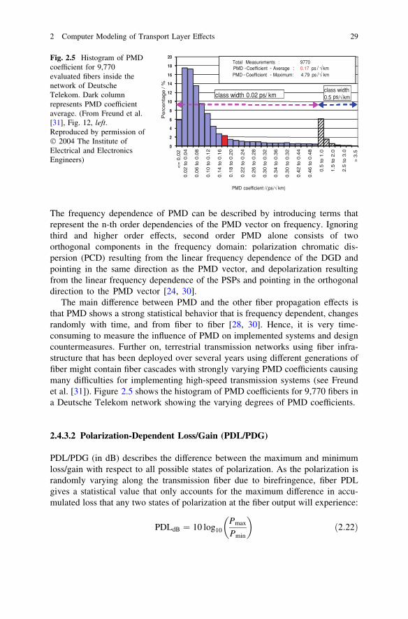
The main difference between PMD and the other fiber propagation effects isthat PMD shows a strong statistical behavior that is frequency dependent, changesrandomly with time, and from fiber to fiber [28, 30]. Hence, it is very time-consuming to measure the influence of PMD on implemented systems and designcountermeasures. Further on, terrestrial transmission networks using fiber infra-structure that has been deployed over several years using different generations offiber might contain fiber cascades with strongly varying PMD coefficients causingmany difficulties for implementing high-speed transmission systems (see Freundet al. [31]). Figure 2.5 shows the histogram of PMD coefficients for 9,770 fibers ina Deutsche Telekom network showing the varying degrees of PMD coefficients.

2.4.3.2 Polarization-Dependent Loss/Gain (PDL/PDG)

PDL/PDG (in dB) describes the difference between the maximum and minimumloss/gain with respect to all possible states of polarization. As the polarization israndomly varying along the transmission fiber due to birefringence, fiber PDLgives a statistical value that only accounts for the maximum difference in accu-mulated loss that any two states of polarization at the fiber output will experience:

PDLdB ¼ 10 log10Pmax

Pmin

� �ð2:22Þ

coefficient / km)

Total Measurements : 9770PMD-Coefficient Average 0.17 ps/PMD-Coefficient Maximum: 4.79 ps/ km

ps km

0

2

4

6

8

10

12

14

16

18

20

<=

0,0

2

0.0

2 t

o 0

.04

0.0

6 t

o 0

.08

0.1

0 t

o 0

.12

0.1

4 t

o 0

.16

0.1

8 t

o 0

.20

0.2

2 t

o 0

.24

0.2

6 t

o 0

.28

0.3

0 t

o 0

.32

0.3

4 t

o 0

.36

0.3

0 t

o 0

.32

0.4

2 t

o 0

.44

0.4

6 t

o 0

.48

0.5

to

1.0

1.5

to

2.0

2.5

to

3.0

> 3

.5

PMD (ps/√

Perc

enta

ge

/ %

Total Measurements : 9770PMD -Coefficient - Average : 0.17 ps / √kmPMD - Coefficient - Maximum: 4.79 ps /√ km

class width 0.02 ps/ kmclass width0.5 ps/√km

Fig. 2.5 Histogram of PMDcoefficient for 9,770evaluated fibers inside thenetwork of DeutscheTelekom. Dark columnrepresents PMD coefficientaverage. (From Freund et al.[31], Fig. 12, left.Reproduced by permission of� 2004 The Institute ofElectrical and ElectronicsEngineers)


with Pmax and Pmin being the measured output powers. Note that those two statesof polarization always represent orthogonal polarizations [32].

Although the PDL of modern transmission fibers is rather small, and mostlynegligible, the PDL of individual components or discrete events along the trans-mission line (such as couplers, splices, filters) can cause significant power fluc-tuations with respect to polarization. Furthermore, optical amplifiers such asErbium-doped fiber amplifiers (EDFA), semiconductor optical amplifiers (SOA)and fiber Raman amplifiers (FRA) or distributed Raman amplifiers (DRA) ascommonly referred to may provide unequal gain for all states of polarization, aneffect referred to as PDG. The definition for PDG is similar to that of PDL inEq. 2.22.

Generally, the PDL (or PDG) of concatenated components cannot be deter-mined by just adding the PDL of the individual components as the state ofpolarization of each PDL-element is different due to the random birefringence ofthe fiber links connecting these individual components. Consequently, thisapproximation would give a far too pessimistic number (as it assumes all PDLelements are polarization aligned). A statistical modeling approach is moreappropriate in order to estimate the average PDL value and its variation for agiven link. It has been found that for a link with many individual PDL elements,the PDF of the overall PDL at the output of that link can be approximated wellby a Maxwellian distribution [33]. Additionally, attention needs to be paid to thefact that in combination with PMD, PDL (and PDG) can produce significantamounts of signal distortions, and thus, limit the system reach (see for instance[34–37]).

2.4.3.3 Polarization-Dependent Kerr

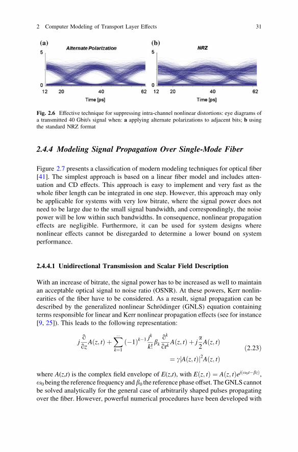
Fiber Kerr nonlinearities—resulting in inter-channel (SPM, XPM, FWM) andintra-channel (I-XPM, I-FWM) propagation effects—are actually polarization-dependent. For example, XPM causes nonlinear polarization rotation of theStokes vector of the propagating channels as shown in Wang and Menyuk [38].The knowledge of the polarization dependence of Kerr nonlinearities can also beused favorably in transmission system design (see for example [39, 40]).Figure 2.6 shows two eye diagrams demonstrating an effective technique forsuppressing intra-channel nonlinear distortions by sending adjacent bits inalternate polarizations. Here, results are shown for a 40 Gbit/s NRZ signal aftertransmission over a 2,500 km dispersion-compensated fiber link. Clearly, thecase using alternate polarization (see Fig. 2.6a) shows much less inter-symboldegradations (here mainly due to I-XPM) compared to the case using standardNRZ modulation (see Fig. 2.6b). Similarly, adjacent WDM channels are oftenlaunched in orthogonal polarizations to reduce inter-channel nonlinear interac-tions between them.

30 A. Richter

2.4.4 Modeling Signal Propagation Over Single-Mode Fiber

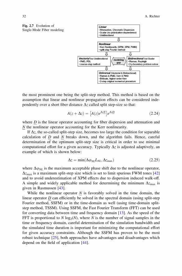
Figure 2.7 presents a classification of modern modeling techniques for optical fiber[41]. The simplest approach is based on a linear fiber model and includes atten-uation and CD effects. This approach is easy to implement and very fast as thewhole fiber length can be integrated in one step. However, this approach may onlybe applicable for systems with very low bitrate, where the signal power does notneed to be large due to the small signal bandwidth, and correspondingly, the noisepower will be low within such bandwidths. In consequence, nonlinear propagationeffects are negligible. Furthermore, it can be used for system designs wherenonlinear effects cannot be disregarded to determine a lower bound on systemperformance.

2.4.4.1 Unidirectional Transmission and Scalar Field Description

With an increase of bitrate, the signal power has to be increased as well to maintainan acceptable optical signal to noise ratio (OSNR). At these powers, Kerr nonlin-earities of the fiber have to be considered. As a result, signal propagation can bedescribed by the generalized nonlinear Schrödinger (GNLS) equation containingterms responsible for linear and Kerr nonlinear propagation effects (see for instance[9, 25]). This leads to the following representation:

jo

ozAðz; tÞ þ

X...

k¼1

ð�1Þk�1 jk

k!bk

ok

otkAðz; tÞ þ j

a2

Aðz; tÞ

¼ c Aðz; tÞj j2Aðz; tÞð2:23Þ

where A(z,t) is the complex field envelope of E(z,t), with Eðz; tÞ ¼ Aðz; tÞejðx0t�bzÞ,x0 being the reference frequency and b0 the reference phase offset. The GNLS cannotbe solved analytically for the general case of arbitrarily shaped pulses propagatingover the fiber. However, powerful numerical procedures have been developed with

Fig. 2.6 Effective technique for suppressing intra-channel nonlinear distortions: eye diagrams ofa transmitted 40 Gbit/s signal when: a applying alternate polarizations to adjacent bits; b usingthe standard NRZ format


the most prominent one being the split-step method. This method is based on theassumption that linear and nonlinear propagation effects can be considered inde-pendently over a short fiber distance Dz called split step-size so that:

Aðzþ DzÞ ¼ AðzÞeDzN� �

eDzD ð2:24Þ

where D is the linear operator accounting for fiber dispersion and attenuation andN the nonlinear operator accounting for the Kerr nonlinearity.

If Dz, the so-called split-step size, becomes too large the condition for separablecalculation of D and N breaks down, and the algorithm fails. Hence, carefuldetermination of the optimum split-step size is critical in order to use minimalcomputational effort for a given accuracy. Typically Dz is adjusted adaptively, anexample of which is shown below:

Dz ¼ min DuNLLNL;Dzmaxð Þ ð2:25Þ

where DuNL is the maximum acceptable phase shift due to the nonlinear operator,Dzmax is a maximum split-step size which is set to limit spurious FWM tones [42]and to avoid underestimation of XPM effects due to dispersion induced walk-off.A simple and widely applicable method for determining the minimum Dzmax isgiven in Rasmussen [43].

While the nonlinear operator N is favorably solved in the time domain, thelinear operator D can efficiently be solved in the spectral domain (using split-stepFourier method, SSFM) or in the time-domain as well (using time-domain split-step method, TSSM). Using SSFM, the Fast Fourier Transform (FFT) can be usedfor converting data between time and frequency domain [13]. As the speed of theFFT is proportional to N log2(N), where N is the number of signal samples in thetime or frequency domain, careful determination of the simulation bandwidth andthe simulated time duration is important for minimizing the computational effortfor given accuracy constraints. Although the SSFM has proven to be the mostrobust technique [25], both approaches have advantages and disadvantages whichdepend on the field of application [44].

Fig. 2.7 Evolution ofSingle-Mode Fiber modeling

32 A. Richter

For small simulation bandwidths and systems with low amounts of accumulateddispersions a TSSM that uses infinite impulse response (IIR) calculations to solveD is more efficient than the SSFM (see Fig. 2.4 in Carena et al. [45]) consideringsome modeling approximations. Generally, this applies also to other TSSM using,for instance, overlap-and-add (OAA) to solve D [46]. The main advantage ofTSSMs in an environment with an aperiodic representation of the time domain isthat the data sequence can be divided easily into small blocks which are handledsequentially. However, the Singleton method [47] can be applied in an SSFM todivide the size of Fourier Transforms into smaller blocks as well. Doing this,simulation speed can be increased by parallelizing the computation effort in bothcases. The walk-off between channels in a WDM system becomes significant forhigher amounts of accumulated CD and a large simulation bandwidth, and thus,a relatively long bit sequence must be chosen for system performance analysiswhen using time-domain approaches with aperiodic representations. One furtherproblem is associated with the buildup time of IIR filters or virtual signal delays incase of OAA methods. Simulation data generated during such buildup time mustbe removed before the system performance is estimated.

These problems do not exist in the case of the SSFM. Here, the problem withdifferent group velocities is eradicated because of the periodic time-domain rep-resentation of signals. For example, channels that are delayed in the simulationwill be ‘wrapped-around’ to the beginning of the data block: no energy is lost, andthe wrap-around represents exactly the data delayed from earlier in the actual datasequence. Note that this artificial periodicity may affect the measured signal sta-tistics, so one should carefully check potential correlations and select the simulatedtime duration to be long enough. Furthermore, the frequency-dependent phase shiftcaused by CD is exactly represented using SSFM, not only approximated by atruncated filter impulse response when using TSSM. In time domain, this can beunderstood as wrapping around an infinite impulse response within the periodicblock of samples. This is accurate over all frequencies, whereas TSSM introducesinaccuracies close to the edges of the modeled bandwidth due to truncation effects(Gibb’s phenomenon as shown in Oppenheim and Schafer [13]). SSFM also showsadvantages when modeling dispersion-limited optical systems with vanishingnonlinearity. Here only a single step (equal to the total fiber length) is required.This greatly accelerates computation effort compared to time-domain techniquesfor solving the linear operator D. Finally, the flexibility is a very important issuethat should be taken into account when choosing the simulation domain. Forexample, it is much more difficult to include a realistic dispersion dependency onfrequency or the Raman response function into the TSSM than to the SSFM. Anychanges of the equations adding higher order derivatives would usually lead to amajor rework of time-domain algorithms.

To make simulations of wideband systems even more effective, the SSFM canbe extended for the GNLS to accept PS and NBs, and to allow individual samplingof spectrally non-overlapping signals. This approach is often referred to as fre-quency decomposition (FD) method or mean-field approach [48] and can be usedas the main tool for multi-band WDM system simulations at moderate bitrates.


2.4.4.2 Unidirectional Transmission and Vectorial Field Description

An increase of the channel bitrate to more than 10 Gbit/s makes degradations dueto PMD noticeable. Modeling PMD in the fiber requires a vectorial approach,describing the electrical field of the propagating light by its Jones vector, and notonly by the SOP-averaged electrical field components. To simulate systemdegradations due to PMD is time-consuming, as PMD is a random phenomenonthat is varying in time and frequency. Special statistical treatments such as thecoarse-step model [49, 50] (possibly combined with the importance samplingtechnique [51]) can be applied to avoid an inefficient straightforward integrationwith very short steps accounting for the short scale length of PMD. Using thesetechniques, simulations of specific fiber conditions become possible in reasonabletime. However, many of those simulation runs are still required to determinestatistical information about polarization-dependent fiber characteristics.

Besides statistical modeling of all orders of PMD, the fiber model shall considerKerr nonlinearities and CD as well as their interplay, especially when investigatinghigh-speed transmission systems. For this purpose, a set of modified GNLSequations (similar to Eq. 2.23) for the two orthogonal polarization components ofthe electrical field E(z, t)x,y can be used to describe propagation mechanisms overbirefringent optical fibers [52]. Assuming rapidly varying birefringence and thatthe polarization states of light average over the whole Poincare sphere, theManakov equation has been derived from that [49], with the coarse-step methodbeing introduced as an efficient numerical method for solving it. Later work thenled to the Manakov-PMD equation [27, 50], which provides a closed-form andnumerically efficiently solvable description of the interplay between CD, Kerr, andPMD effects in optical fiber.

The widely used intuitive coarse-step model, introduced by Wai et al. [49]without strict mathematical reasoning, is based on the assumption that althoughbirefringence perturbations vary from position to position along the fiber length,their impact can be modeled by a concatenation of ‘coarse’ fiber sections, eachlonger than the correlation length Lcorr of the fiber, with randomly rotated PSPs andstep-wise constant birefringence values. For each of these fiber sections the SSFM,or alternatively, TSSM is used to numerically solve the propagation equations. Thelength of each polarization section should be much shorter than the total fiberdistance in order to model a sufficient number of randomly oriented sections.Studies such as Wai and Menyuk [27], Marcuse et al. [50] showed the validity of thecoarse-step model when applied with the correct weighting factors and scatteringoperations between sections for approximating solutions of the polarization-coupled GNLS equations with the precondition that Lcorr and Lb (describing the beatlength as a measure of fiber birefringence as in Kaminow and Li [24]) are muchshorter than LNL. This restriction ensures that the effect of fiber nonlinearity isaveraged over the quick oscillation of the signal state of polarization for eachpolarization section. Consequently, this precondition imposes limitations on thehighest possible signal intensity that can be simulated with this method. However,for typical signals used in telecommunications this condition is well satisfied.

34 A. Richter

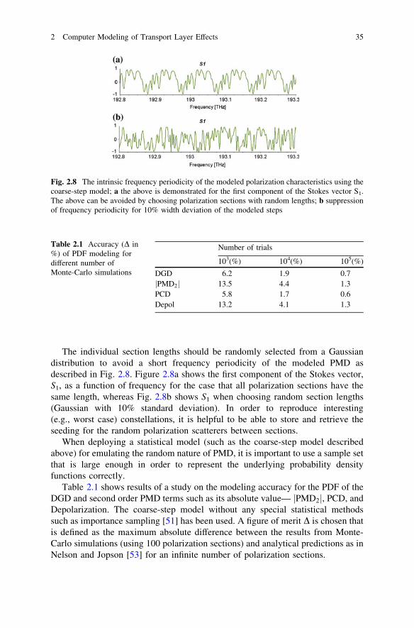
The individual section lengths should be randomly selected from a Gaussiandistribution to avoid a short frequency periodicity of the modeled PMD asdescribed in Fig. 2.8. Figure 2.8a shows the first component of the Stokes vector,S1, as a function of frequency for the case that all polarization sections have thesame length, whereas Fig. 2.8b shows S1 when choosing random section lengths(Gaussian with 10% standard deviation). In order to reproduce interesting(e.g., worst case) constellations, it is helpful to be able to store and retrieve theseeding for the random polarization scatterers between sections.

When deploying a statistical model (such as the coarse-step model describedabove) for emulating the random nature of PMD, it is important to use a sample setthat is large enough in order to represent the underlying probability densityfunctions correctly.

Table 2.1 shows results of a study on the modeling accuracy for the PDF of theDGD and second order PMD terms such as its absolute value— PMD2j j, PCD, andDepolarization. The coarse-step model without any special statistical methodssuch as importance sampling [51] has been used. A figure of merit D is chosen thatis defined as the maximum absolute difference between the results from Monte-Carlo simulations (using 100 polarization sections) and analytical predictions as inNelson and Jopson [53] for an infinite number of polarization sections.

Fig. 2.8 The intrinsic frequency periodicity of the modeled polarization characteristics using thecoarse-step model; a the above is demonstrated for the first component of the Stokes vector S1.The above can be avoided by choosing polarization sections with random lengths; b suppressionof frequency periodicity for 10% width deviation of the modeled steps

Table 2.1 Accuracy (D in%) of PDF modeling fordifferent number ofMonte-Carlo simulations

Number of trials

103(%) 104(%) 105(%)

DGD 6.2 1.9 0.7PMD2j j 13.5 4.4 1.3

PCD 5.8 1.7 0.6Depol 13.2 4.1 1.3


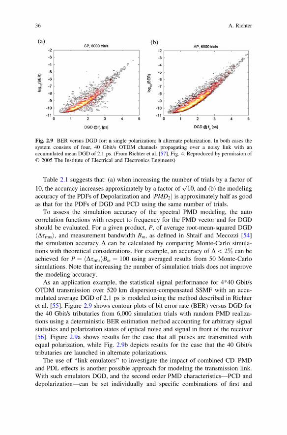
Table 2.1 suggests that: (a) when increasing the number of trials by a factor of10, the accuracy increases approximately by a factor of

ffiffiffiffiffi10p

, and (b) the modelingaccuracy of the PDFs of Depolarization and PMD2j j is approximately half as goodas that for the PDFs of DGD and PCD using the same number of trials.

To assess the simulation accuracy of the spectral PMD modeling, the autocorrelation functions with respect to frequency for the PMD vector and for DGDshould be evaluated. For a given product, P, of average root-mean-squared DGDDsrmsh i, and measurement bandwidth Bm, as defined in Shtaif and Mecozzi [54]

the simulation accuracy D can be calculated by comparing Monte-Carlo simula-tions with theoretical considerations. For example, an accuracy of D\ 2% can beachieved for P ¼ Dsrmsh iBm ¼ 100 using averaged results from 50 Monte-Carlosimulations. Note that increasing the number of simulation trials does not improvethe modeling accuracy.

As an application example, the statistical signal performance for 4*40 Gbit/sOTDM transmission over 520 km dispersion-compensated SSMF with an accu-mulated average DGD of 2.1 ps is modeled using the method described in Richteret al. [55]. Figure 2.9 shows contour plots of bit error rate (BER) versus DGD forthe 40 Gbit/s tributaries from 6,000 simulation trials with random PMD realiza-tions using a deterministic BER estimation method accounting for arbitrary signalstatistics and polarization states of optical noise and signal in front of the receiver[56]. Figure 2.9a shows results for the case that all pulses are transmitted withequal polarization, while Fig. 2.9b depicts results for the case that the 40 Gbit/stributaries are launched in alternate polarizations.

The use of ‘‘link emulators’’ to investigate the impact of combined CD–PMDand PDL effects is another possible approach for modeling the transmission link.With such emulators DGD, and the second order PMD characteristics—PCD anddepolarization—can be set individually and specific combinations of first and

Fig. 2.9 BER versus DGD for: a single polarization; b alternate polarization. In both cases thesystem consists of four, 40 Gbit/s OTDM channels propagating over a noisy link with anaccumulated mean DGD of 2.1 ps. (From Richter et al. [57], Fig. 4. Reproduced by permission of� 2005 The Institute of Electrical and Electronics Engineers)

36 A. Richter

second order PMD can be selected. Many other possible implementations havebeen proposed as in Francia et al. [58], Kogelnik et al. [59], Eyal et al. [60],Orlandini and Vincetti [61] which typically differ in the amount of residual thirdand higher order PMD terms that cannot be controlled by the emulator.

2.4.4.3 Bidirectional Transmission and Scalar Field Description

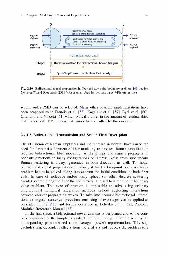
The utilization of Raman amplifiers and the increase in bitrates have raised theneed for further development of fiber modeling techniques. Raman amplificationrequires bidirectional fiber modeling, as the pumps and signals propagate inopposite directions in many configurations of interest. Noise from spontaneousRaman scattering is always generated in both directions as well. To modelbidirectional signal propagations in fibers, at least a two-point boundary valueproblem has to be solved taking into account the initial conditions at both fiberends. In case of reflective and/or lossy splices (or other discrete scatteringevents) located along the fiber the complexity is raised to a multipoint boundaryvalue problem. This type of problem is impossible to solve using ordinaryunidirectional numerical integration methods without neglecting interactionsbetween counter-propagating waves. To take into account bidirectional interac-tions an original numerical procedure consisting of two stages can be applied aspresented in Fig. 2.10 and further described in Poloyko et al. [62], PhotonicModules Reference Manual [63].

In the first stage, a bidirectional power analysis is performed and so the com-plex amplitudes of the sampled signals at the input fiber ports are replaced by thecorresponding parameterized (time-averaged power) representation. This stepexcludes time-dependent effects from the analysis and reduces the problem to a

Fig. 2.10 Bidirectional signal propagation in fiber and two-point boundary problem, [63, sectionUniversalFiber] (Copyright 2011 VPIsystems. Used by permission of VPIsystems Inc)


two-point boundary value problem for ordinary differential equations describingthe signal power propagation along the fiber. The corresponding two-pointboundary value problem can effectively be solved by an iterative algorithm.Simulation accuracy and speed depend strongly on the frequency discretizationthat is applied for this approximation process. It is useful in practical calculationsto specify different resolutions for frequency regions containing sampled datasignals and other regions, only containing optical noise.

In the second stage, the optical field analysis can be performed by firstsubstituting the power distributions in both directions along the fiber distance thathave been found after completing the first step into the full GNLS equation(see Eq. 2.23). With this substitution, terms including counter-propagating signalpowers become defined everywhere along the fiber. This approach is possibleassuming that dynamic (time and pulse shape-dependent) propagation effectsinduced by interactions of counter-propagating waves are negligible. As theirinteraction time is very short only the spatially resolved average power of counter-propagating signals is of relevance. Furthermore, it can be assumed that FWMbetween counter-propagating waves is negligible due to the phase mismatch. As aresult, the two-point boundary problem reduces to a problem similar to the uni-directional propagation, and the SSFM can be used for effectively solving it.Depending on the specific application, the field analysis performed in the secondstep could be done for frequency bands propagating in the forward, in the back-ward, or in both directions.

When modeling bidirectional propagation effects over heterogeneous fiber linksconsisting of several different fiber spans it is important to consider each span byits individual fiber characteristics (e.g., attenuation, CD, Rayleigh coefficient,nonlinear index, core area, Raman gain etc.) and to add information about lossesand reflections at fiber splices and fiber ends.

For an accurate modeling of wideband applications it is important to account forthe wavelength-dependence of relevant fiber properties as well. For instance, theRaman gain profile of the fiber needs to be known when modeling SRS. As theRaman gain depends on the pump frequency, either many profiles measured atdifferent pump wavelengths are to be supplied and the actual Raman gain at thefrequencies of interest is obtained by interpolation, or Raman gains at differentpump wavelengths should be approximated using correct frequency scaling [62, 64].

Even more care is needed when trying to adjust multiple pumps at differentwavelengths in order to achieve flat amplification over a wide spectral width.Special optimization algorithms are needed for this task due to the large number ofopen parameters [65, 66]. To make those optimization algorithms applicable forreal-world problems, it is essential that they consider not only all Raman-relatedpropagation effects, but also other power-related effects along the fiber. Forinstance, signal–signal Raman interactions, Rayleigh and Brillouin scattering, andpower-related variations of broadband pump sources can cause significantamplifier degradations [67].

The possibility to model the different physical effects individually or in com-bination, and to control their strengths is important for the assessment of sources

38 A. Richter

for system degradations (and saving computation time). Further on, adjustmentfactors could be introduced to scale the strength of nonlinear interactions due toSPM, XPM, and SRS between co-propagating bands. These factors can forinstance, account for the dependence of Raman interactions on the mutualpolarization of the interacting fields, for example: when using information that wasobtained by measuring the Raman gain coefficient for a short (*meters) fiber withco-polarized signal and pump, an adjustment factor of 0.5 should be used in orderto treat the Raman gain correctly; when simulating long (*100 km) fiber spans,the polarizations of pump and signals vary randomly with respect to each other dueto the frequency-dependence of PMD. As another example indicates, the SPMeffect can be scaled by the factor 8/9 to account for the averaging of Kerr non-linearities for applications where PMD and PDL can be neglected, if the value ofnonlinear index coefficient n2 used for the simulations has been measured withoutconsidering polarization averaging over long fibers [25]. Similarly, the XPM effectbetween orthogonally polarized signals propagating in different sampled bandsover high-birefringence fiber can be scaled accordingly to account for the fact thatXPM is much stronger for signals with aligned polarizations.

2.4.4.4 Bidirectional Transmission and Vectorial Field Description

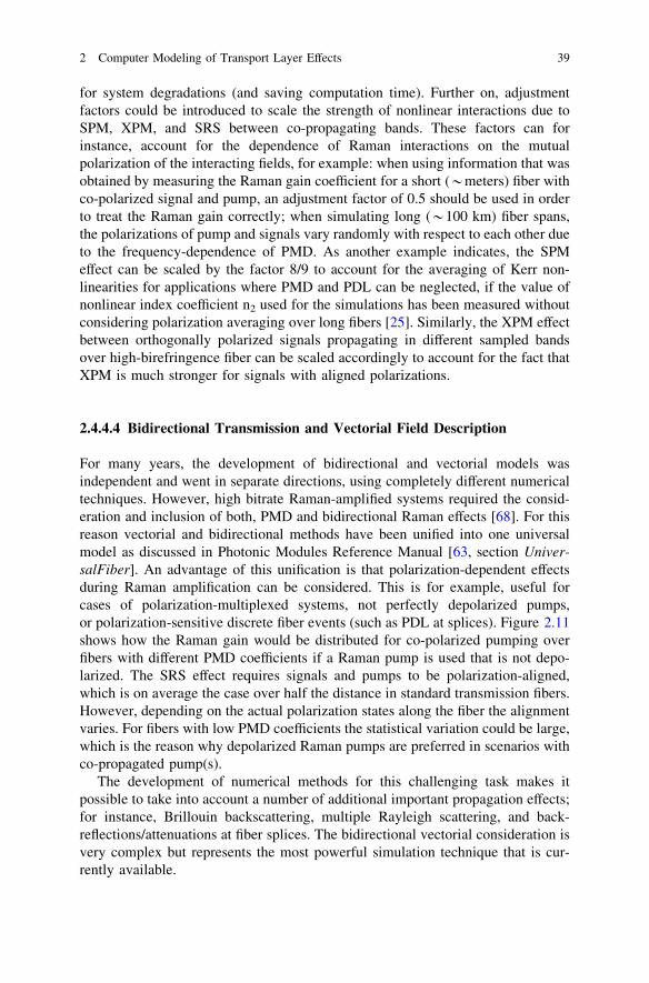
For many years, the development of bidirectional and vectorial models wasindependent and went in separate directions, using completely different numericaltechniques. However, high bitrate Raman-amplified systems required the consid-eration and inclusion of both, PMD and bidirectional Raman effects [68]. For thisreason vectorial and bidirectional methods have been unified into one universalmodel as discussed in Photonic Modules Reference Manual [63, section Univer-salFiber]. An advantage of this unification is that polarization-dependent effectsduring Raman amplification can be considered. This is for example, useful forcases of polarization-multiplexed systems, not perfectly depolarized pumps,or polarization-sensitive discrete fiber events (such as PDL at splices). Figure 2.11shows how the Raman gain would be distributed for co-polarized pumping overfibers with different PMD coefficients if a Raman pump is used that is not depo-larized. The SRS effect requires signals and pumps to be polarization-aligned,which is on average the case over half the distance in standard transmission fibers.However, depending on the actual polarization states along the fiber the alignmentvaries. For fibers with low PMD coefficients the statistical variation could be large,which is the reason why depolarized Raman pumps are preferred in scenarios withco-propagated pump(s).

The development of numerical methods for this challenging task makes itpossible to take into account a number of additional important propagation effects;for instance, Brillouin backscattering, multiple Rayleigh scattering, and back-reflections/attenuations at fiber splices. The bidirectional vectorial consideration isvery complex but represents the most powerful simulation technique that is cur-rently available.


In summary, the ultimate (universal) model for single-mode fiber propagationsupports

• the modeling of wideband bidirectional transmission and interaction of signals,pumps, and noise

• the representation of signals, pumps and noise by sampled waveforms or time-aver-aged parameters (e.g., to keep them separately and increase simulation efficiency), and

• the wavelength-dependent definition of all fiber parameters (attenuation, CD,effective mode area, nonlinear coefficient, Brillouin and Raman scatteringresponses, Rayleigh backscattering, birefringence profile, etc.)

The full vector model (Jones) for arbitrary polarization dependencies and thescalar model (SOP averaging) for a linear polarized approximation define the mainmodes of operation. In scalar mode, the universal model shall include attenuation,CD, Kerr nonlinearities with delayed-response terms, SRS between pumps, signalsand noise, point reflections and losses, Raman-induced changes of the nonlinearrefractive index, wideband noise generation due to spontaneous Raman scatteringat any temperature, stimulated and spontaneous Brillouin scattering including thelinewidth-dependence of the reflection coefficient, and multiple Rayleigh scatter-ing. In vectorial mode, the model shall additionally be able to account for all-orderPMD (with optional techniques to weight statistics and emphasize less likelyevents), and polarization dependencies of nonlinear Kerr and scattering effects.

Furthermore, it is very helpful to have the ability to switch individual propa-gation effects on/off and to define heterogeneous fibers consisting of multiplespans of different fiber types that are connected by lossy and reflective splices.Parameters that control the numerical accuracy and calculation speed of under-lying algorithms as well as means for visualizing fiber characteristics versusdistance or frequency and the numerical convergence of calculation algorithms arealso extremely important and helpful.

2.4.4.5 Parametric Analysis

While a high level of detail is important for component and subsystem design, rapidvisualization of important performance measures can aid in the overall understandingof systems, and thus, be very useful in system and network design. In conjunctionwith approximate design rules network engineers can access, without demonstrating

Fig. 2.11 Distributions ofRaman gain for fibers withdifferent PMD coefficientsusing a single co-propagatedRaman pump withoutdepolarization. (Note: 0 dBgain corresponds to perfectcompensation of fiber loss forthe case that a depolarizedpump is used)

40 A. Richter

very detailed photonics knowledge, whether a network (or sub-network) is likely tooperate properly or not. Such a quick performance assessment can be achieved usinga parametric approach that avoids time-consuming simulation runs when verifyingcomplex network configurations and identifying potential design flaws [69].

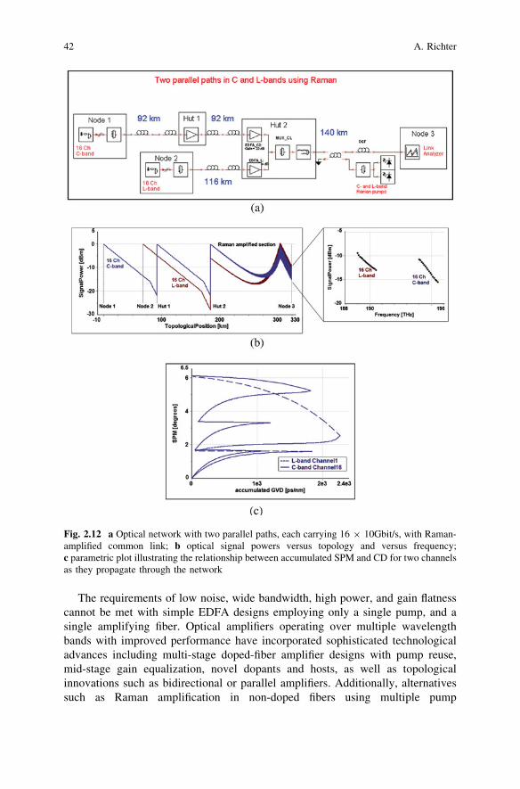
Figure 2.12 shows a sample network configuration and typical results of theparametric system validation process. Figure 2.12a depicts the simulation setup1

of a three-node network that consists of two parallel paths connecting N1 and N2with H2, and a common Raman-amplified 140 km link connecting H2 with N3.A total of 16 C-band channels each carrying 10 Gbit/s are used for communicationbetween N1 and N3, while 16 L-band channels are deployed between N2 and N3.The individual SSMF fiber spans are post-compensated by appropriate DCFs;EDFAs are placed at H1 and H2 accounting for the accumulated loss. Figure 2.12bshows optical signal powers versus topology (left) and versus frequency at N3(right). Figure 2.12c shows a parametric plot illustrating the relationship betweenaccumulated SPM and CD for two channels (one in C-band and one in L-band) asthey propagate through the network. Without the need to run detailed simulationsthe results depicted in Fig. 2.12 indicate that one Raman pump per band is notsufficient to achieve flat gain and the power in both bands is very unbalancedrequiring additional gain adjustments before entering into any possible links thatare following. Furthermore, the designer is able to locate places where largeamounts of accumulated CD and nonlinear phase shift occur simultaneously,something that can lead to significant penalties. Hence, the example discussedabove emphasizes quickly the limitations of the chosen amplification and dis-persion maps.

2.5 Optical Amplification

Several technologies for optical amplification have been introduced over theyears addressing different system requirements and applications: semiconductoroptical amplifiers (SOA), rare earth ion doped fiber (or waveguide) amplifiers(e.g., Erbium-doped fiber amplifier—EDFA), and discrete and distributed fiberRaman amplifiers (FRA). Especially with the invention of the EDFA in the late1980s the development of fiber-optic communication systems accelerated rapidly[70]. Electro-optic repeaters could be replaced by the more robust, flexible, andcost-efficient EDFAs. The main requirements on EDFA technologies from asystems design perspective are: operation over wide wavelength ranges, highoutput powers, equal gain to each channel, low-noise characteristics, negligiblecrosstalk between channels, mechanisms for gain control, high energy efficiency,and low cost.

1 using VPItransmissionMakerTMOptical Systems, Version 8.6.


The requirements of low noise, wide bandwidth, high power, and gain flatnesscannot be met with simple EDFA designs employing only a single pump, and asingle amplifying fiber. Optical amplifiers operating over multiple wavelengthbands with improved performance have incorporated sophisticated technologicaladvances including multi-stage doped-fiber amplifier designs with pump reuse,mid-stage gain equalization, novel dopants and hosts, as well as topologicalinnovations such as bidirectional or parallel amplifiers. Additionally, alternativessuch as Raman amplification in non-doped fibers using multiple pump

Fig. 2.12 a Optical network with two parallel paths, each carrying 16 9 10Gbit/s, with Raman-amplified common link; b optical signal powers versus topology and versus frequency;c parametric plot illustrating the relationship between accumulated SPM and CD for two channelsas they propagate through the network

42 A. Richter

wavelengths and cascaded pumping have been introduced to increase the ampli-fiable system bandwidth and required repeater spacing.

Obviously there are many combinations of amplifier topology, fiber, pump andpassive component technology that could produce a cost-effective, low-noise,wide-bandwidth, high-power, spectrally flat, and power-efficient amplifier.A detailed discussion on the theory and design of EDFAs is given in Desurvire[71], Becker et al. [72]. In what follows we present the main theoretical conceptsand underlying fundamental operating principles for these devices that are inten-ded to facilitate their modeling. In Chap. 3 a ‘‘black-box’’ approach for theirmodeling is also presented.

2.5.1 EDFA Theory

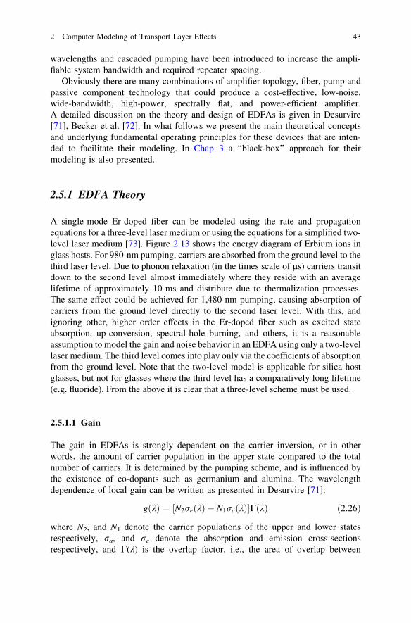
A single-mode Er-doped fiber can be modeled using the rate and propagationequations for a three-level laser medium or using the equations for a simplified two-level laser medium [73]. Figure 2.13 shows the energy diagram of Erbium ions inglass hosts. For 980 nm pumping, carriers are absorbed from the ground level to thethird laser level. Due to phonon relaxation (in the times scale of ls) carriers transitdown to the second level almost immediately where they reside with an averagelifetime of approximately 10 ms and distribute due to thermalization processes.The same effect could be achieved for 1,480 nm pumping, causing absorption ofcarriers from the ground level directly to the second laser level. With this, andignoring other, higher order effects in the Er-doped fiber such as excited stateabsorption, up-conversion, spectral-hole burning, and others, it is a reasonableassumption to model the gain and noise behavior in an EDFA using only a two-levellaser medium. The third level comes into play only via the coefficients of absorptionfrom the ground level. Note that the two-level model is applicable for silica hostglasses, but not for glasses where the third level has a comparatively long lifetime(e.g. fluoride). From the above it is clear that a three-level scheme must be used.

2.5.1.1 Gain

The gain in EDFAs is strongly dependent on the carrier inversion, or in otherwords, the amount of carrier population in the upper state compared to the totalnumber of carriers. It is determined by the pumping scheme, and is influenced bythe existence of co-dopants such as germanium and alumina. The wavelengthdependence of local gain can be written as presented in Desurvire [71]:

gðkÞ ¼ ½N2reðkÞ � N1raðkÞ�CðkÞ ð2:26Þ

where N2, and N1 denote the carrier populations of the upper and lower statesrespectively, ra, and re denote the absorption and emission cross-sectionsrespectively, and C(k) is the overlap factor, i.e., the area of overlap between


http://dx.doi.org/10.1007/978-1-4614-1093-5_3

http://dx.doi.org/10.1007/978-1-4614-1093-5_3

Erbium ions and the optical signal mode in the doped fiber. Note that the popu-lation inversion shows a strong local dependence so gain may differ over the lengthof the doped fiber.

Figure 2.14 shows simulation results characterizing the performance of a singlestage EDFA for different pumping schemes. Figure 2.14a shows amplifier gain asa function of population inversion around the 980 nm (pump) wavelength. Perfectinversion is possible as the emission cross-section is zero at 980 nm. This results insmall noise generation for 980 nm pumped EDFA configurations. Figure 2.14bshows gain as a function of population inversion at 1,480 nm (pump) and around1,550 nm (C-band). For the depicted inversion profile, the transparency point(g = 0 dB/m) for 1,480 nm pumping is at about 75% population inversion.So, perfect inversion is not possible, which results in increased noise generation.The figure depicts the strong wavelength dependence of the gain, which resultsfrom the wavelength dependence of population inversion.

Ignoring noise to begin with, the average signal power dependence on dopedfiber length is given by

dP

dz¼ gðk;PÞP ð2:27Þ

For small signal powers, the total amplifier gain is usually independent of theincoming power. If the power launched into the doped fiber is increased over acertain level, stimulated recombination starts to affect carrier population inversion.Every photon created by stimulated emission transfers one ion from the upper stateto the lower state. This results in gain reduction until absorption of pump powerand stimulated plus spontaneous emissions are balancing each other. This effect isknown as gain saturation. The saturation characteristic of an EDFA is verycomplex, as it is dependent on fiber distance. Assuming a homogeneous powerdistribution along the EDFA, the ratio of input power Pin and saturation power Psat

is given by Iannone et al. [25]

Fig. 2.13 Transitionsbetween energy levels in anEDFA as presented in User’sManual [74, pp. 12](Copyright 2011 VPIsystems.Used by permission ofVPIsystems Inc)

44 A. Richter

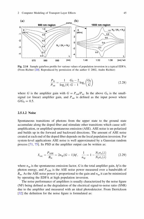
Pin

Psat

¼ 1logeð4Þ

G0 � 2G� 1

logeG0

G

� �ð2:28Þ

where G is the amplifier gain with G = Pout/Pin. In the above G0 is the small-signal (or linear) amplifier gain, and Psat is defined as the input power whereG/G0 = 0.5.

2.5.1.2 Noise

Spontaneous transitions of photons from the upper state to the ground stateaccumulate along the doped fiber and stimulate other transitions which cause self-amplification, or amplified spontaneous emission (ASE). ASE noise is un-polarizedand builds up in the forward and backward directions. The amount of ASE noisecreated at each end of the doped fiber depends on the local population inversion. Forsystem-level applications ASE noise is well approximated by a Gaussian randomprocess [71, 75]. Its PSD at the amplifier output can be written as:

SASE¼ PASE

Bm¼ 2nspðG� 1Þhf ;

1nsp

¼ 1� N1raðkÞN2reðkÞ

ð2:29Þ

where nsp is the spontaneous emission factor, G is the total amplifier gain, hf is thephoton energy, and PASE is the ASE noise power measured over a bandwidth ofBm. As the ASE noise power is proportional to the gain and nsp it can be minimizedby operating the EDFA at high population inversion.

The noise performance of amplifiers is usually characterized by the noise figure(NF) being defined as the degradation of the electrical signal-to-noise ratio (SNR)due to the amplifier and measured with an ideal photodetector. From Derrickson[32] the definition for the noise figure is formulated as:

Fig. 2.14 Sample gain/loss profile for various values of population inversion in a typical EDFA.(From Richter [20]. Reproduced by permission of the author � 2002, Andre Richter)


NF ¼ SNRin

SNRout

� 2nsp

G� 1Gþ 1

Gð2:30Þ

where it is assumed that the ASE–ASE beat noise component can be neglected[76]. With this, the noise PSD can be written as a function of the NF and the gain:

SASE � ðNF G� 1Þhf ð2:31Þ

where both values (NF and gain) are being calculated without knowledge of theinternal architecture of the optical amplifier. Practical EDFA designs consisttypically of multiple stages where the first stage operates as a low-noise pre-amplifier, preferably pumped at 980 nm to ensure small NF. This is advantageousas according to the chain rule, the noise figure of an amplifier cascade is mainlydetermined by the NF of the first amplifier in the chain [77]. The following stagesoperate as a power amplifier, preferably pumped at 1,480 nm as this conceptprovides higher power conversion efficiency. Isolators being placed betweenstages prevent saturation of the previous stages due to backward propagating ASEnoise from the following stage. Also, filters are used to suppress ASE noise outsidethe signal bandwidth and perform gain equalization.

2.5.1.3 Optical Signal-To-Noise Ratio

One important performance parameter is the optical signal-to-noise-ratio (OSNR)which is defined as the ratio of optical signal power and optical noise powerwithin a measurement bandwidth Bm. Using Eq. 2.31 above we can derive thefollowing:

OSNR ¼ Pout

SASEBm� Pin

ðNF � 1=GÞ hf Bm; Pout ¼ GPin ð2:32Þ

The OSNR can be directly related to system performance for applications thatare limited by optical noise. For a signal with perfect extinction ratio, assumingthat signal-ASE beat noise and ASE–ASE beat noise dominate the electrical noise(e.g., ignoring thermal and shot noise added by a direct-detection optical receiver)and further assuming that no other propagation effects, such as for example CD,Kerr, and others, deteriorate the eye opening, the Q factor can be easily related tothe OSNR at the input of the optical receiver [24] as follows:

Q ¼ 2 OSNR

ffiffiffiffiffiffiffiffiffiffiffiffiBo=Be

p1þ

ffiffiffiffiffiffiffiffiffiffiffiffiffiffiffiffiffiffiffiffiffiffiffiffi1þ 4OSNRp ð2:33Þ

In the above, Be is the electrical bandwidth of the receiver and Bo is thebandwidth of the optical filter in front of the receiver. For Bm = Bo, the OSNRvalue should be scaled by the factor Bo/Bm. before being used in the Q factor

46 A. Richter

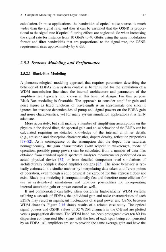
calculation. In most applications, the bandwidth of optical noise sources is muchwider than the signal rate, and thus it can be assumed that the OSNR is propor-tional to the signal rate if optical filtering effects are neglected. So when increasingthe signal rate for instance from 10 Gbit/s to 40 Gbit/s using the same modulationformat and filter bandwidths that are proportional to the signal rate, the OSNRrequirement rises approximately by 6 dB.

2.5.2 Systems Modeling and Performance

2.5.2.1 Black-Box Modeling

A phenomenological modeling approach that requires parameters describing thebehavior of EDFAs in a system context is better suited for the simulation of aWDM transmission line since the internal architecture and parameters of theamplifiers are typically not known at this level of design. For this purposeBlack-Box modeling is favorable. The approach to consider amplifier gain andnoise figure as fixed functions of wavelength is an approximate one since itignores for instance dependencies of pump and signal powers on the EDFA gainand noise characteristics, yet for many system simulation applications it is fairlyadequate.

More accurately, but still making a number of simplifying assumptions on thephysics in the doped fiber, the spectral gain and noise behavior of the EDFA can becalculated requiring no detailed knowledge of the internal amplifier details(e.g., emission and absorption characteristics, dopant density, reflection properties)[78–82]. As a consequence of the assumption that the doped fiber saturateshomogeneously, the gain characteristics (with respect to wavelength, mode ofoperation, possibly pump power) can be calculated from a number of data filesobtained from standard optical spectrum analyzer measurements performed on anactual physical device [32] or from detailed component-level simulations ofarchitecturally complex doped amplifier designs [83]. The noise behavior is typ-ically estimated in a similar manner by interpolating data taken at different pointsof operation, even though a solid physical background for this approach does notexist. Black-box modeling is computationally fast and therefore more efficient foruse in system-level simulations and provides possibilities for incorporatinginternal automatic gain or power control as well.

If not compensated carefully, when designing high-capacity WDM systemsutilizing a cascade of EDFAs, the individual gain and noise characteristics of eachEDFA may result in significant fluctuations of signal power and OSNR betweenWDM channels. Figure 2.15 shows results of a related case study. The opticalsignal powers and OSNR values of 32 WDM channels in the C-Band are plottedversus propagation distance. The WDM band has been propagated over ten 80 kmdispersion compensated fiber spans with the loss of each span being compensatedby an EDFA. All amplifiers are set to provide the same average gain and have the


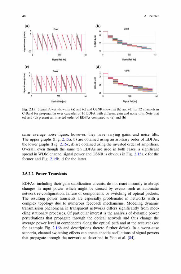
same average noise figure, however, they have varying gains and noise tilts.The upper graphs (Fig. 2.15a, b) are obtained using an arbitrary order of EDFAs;the lower graphs (Fig. 2.15c, d) are obtained using the inverted order of amplifiers.Overall, even though the same ten EDFAs are used in both cases, a significantspread in WDM channel signal power and OSNR is obvious in Fig. 2.15a, c for theformer and Fig. 2.15b, d for the latter.

2.5.2.2 Power Transients

EDFAs, including their gain stabilization circuits, do not react instantly to abruptchanges in input power which might be caused by events such as automaticnetwork re-configuration, failure of components, or switching of optical packets.The resulting power transients are especially problematic in networks with acomplex topology due to numerous feedback mechanisms. Modeling dynamictransmission phenomena in transparent networks differs significantly from mod-eling stationary processes. Of particular interest is the analysis of dynamic powerperturbations that propagate through the optical network and thus change theaverage power level at components along the optical path and at the receiver (seefor example Fig. 2.16b and descriptions thereto further down). In a worst-casescenario, channel switching effects can create chaotic oscillations of signal powersthat propagate through the network as described in Yoo et al. [84].

Fig. 2.15 Signal Power shown in (a) and (c) and OSNR shown in (b) and (d) for 32 channels inC-Band for propagation over cascades of 10 EDFA with different gain and noise tilts. Note that(c) and (d) present an inverted order of EDFAs compared to (a) and (b)

48 A. Richter

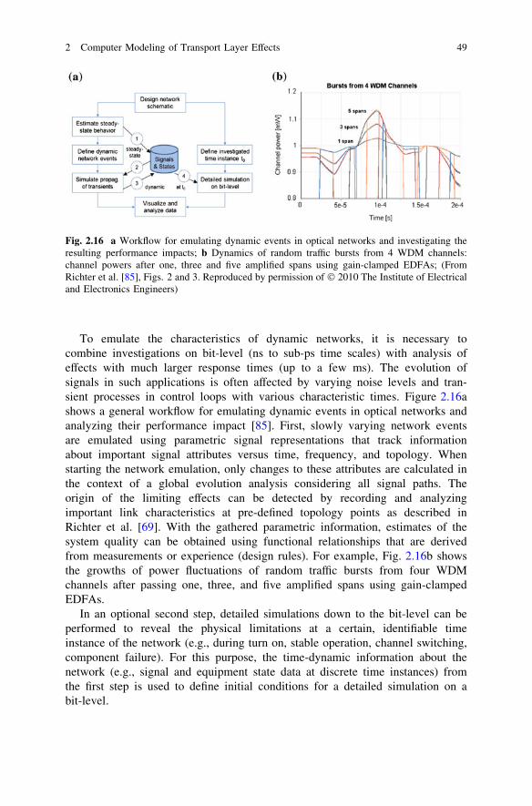
To emulate the characteristics of dynamic networks, it is necessary tocombine investigations on bit-level (ns to sub-ps time scales) with analysis ofeffects with much larger response times (up to a few ms). The evolution ofsignals in such applications is often affected by varying noise levels and tran-sient processes in control loops with various characteristic times. Figure 2.16ashows a general workflow for emulating dynamic events in optical networks andanalyzing their performance impact [85]. First, slowly varying network eventsare emulated using parametric signal representations that track informationabout important signal attributes versus time, frequency, and topology. Whenstarting the network emulation, only changes to these attributes are calculated inthe context of a global evolution analysis considering all signal paths. Theorigin of the limiting effects can be detected by recording and analyzingimportant link characteristics at pre-defined topology points as described inRichter et al. [69]. With the gathered parametric information, estimates of thesystem quality can be obtained using functional relationships that are derivedfrom measurements or experience (design rules). For example, Fig. 2.16b showsthe growths of power fluctuations of random traffic bursts from four WDMchannels after passing one, three, and five amplified spans using gain-clampedEDFAs.

In an optional second step, detailed simulations down to the bit-level can beperformed to reveal the physical limitations at a certain, identifiable timeinstance of the network (e.g., during turn on, stable operation, channel switching,component failure). For this purpose, the time-dynamic information about thenetwork (e.g., signal and equipment state data at discrete time instances) fromthe first step is used to define initial conditions for a detailed simulation on abit-level.

Fig. 2.16 a Workflow for emulating dynamic events in optical networks and investigating theresulting performance impacts; b Dynamics of random traffic bursts from 4 WDM channels:channel powers after one, three and five amplified spans using gain-clamped EDFAs; (FromRichter et al. [85], Figs. 2 and 3. Reproduced by permission of � 2010 The Institute of Electricaland Electronics Engineers)


2.6 Optical Signal Generation

2.6.1 Types of Modulation

The technology of optical transmitters can be divided into two broad categories:transmitters made of a laser that is modulated directly by the electrical drivingsignal carrying the information sequence called directly modulated laser (DML),and transmitters that are combinations of a laser delivering a continuous wave(CW) followed by an external modulator (called externally modulated laser orEML) or a cascade of such devices.

2.6.1.1 Direct Modulation

The applicability of directly modulated lasers in modern transmission systems islimited due to the narrow modulation bandwidth of lasers and the generation offrequency fluctuations with time (chirp) that are hard to control or eliminate.Chirp combined with CD critically affects the channel transmission performanceover fiber. Recent work on chirp-managed lasers (CMLs) has proven that highdispersion tolerance could be achieved when using the directly modulated laser incombination with a carefully tailored optical filter applied to counteract theadiabatic chirp from a laser [86].

The behavior of DMLs is most easily predicted using laser rate equation modelsrequiring physical parameters describing the internal cavity mechanisms of the laser.These physical parameters can be easily estimated by fitting theoretical curves tomeasured data for intensity modulation response, light–current characteristic, andtime-resolved chirp [87]. Simple rate equation models ignore the details of the opticalspectrum (assuming a single-mode, both in the longitudinal and transverse direc-tions). Specifically, distributed feedback (DFB) lasers are well suited for a descriptionby rate equations because the DFB design allows suppressing side modes efficiently.However, in order to evaluate such suppression and design optimal DFB structures,laser models that include the longitudinal structure of the laser such as the trans-mission-line laser model and its variants [88, 89] are required. If the variation of thecarrier density is represented longitudinally these detailed models can predict chirpdue to longitudinal spatial hole burning and even instabilities caused by this effect.

2.6.1.2 External Modulation

WDM transmission systems employing channel bitrates of 10 Gbit/s and highertypically deploy externally modulated transmitters. These provide a high wave-length-stability, small amount of distortions, high extinction ratio, and a definedfrequency chirp characteristic that can be controlled to counteract for fiber prop-agation degradations due to CD and SPM [90]. The laser in an externally

50 A. Richter

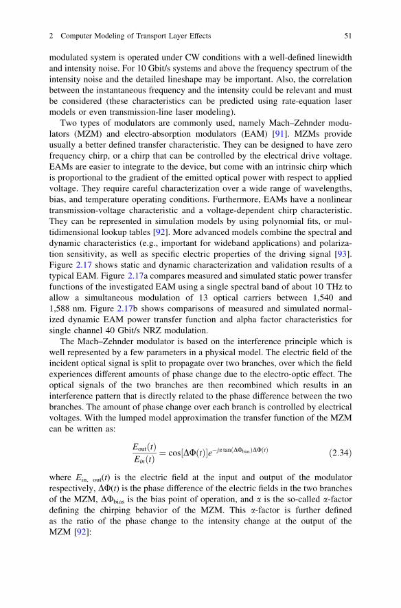
modulated system is operated under CW conditions with a well-defined linewidthand intensity noise. For 10 Gbit/s systems and above the frequency spectrum of theintensity noise and the detailed lineshape may be important. Also, the correlationbetween the instantaneous frequency and the intensity could be relevant and mustbe considered (these characteristics can be predicted using rate-equation lasermodels or even transmission-line laser modeling).

Two types of modulators are commonly used, namely Mach–Zehnder modu-lators (MZM) and electro-absorption modulators (EAM) [91]. MZMs provideusually a better defined transfer characteristic. They can be designed to have zerofrequency chirp, or a chirp that can be controlled by the electrical drive voltage.EAMs are easier to integrate to the device, but come with an intrinsic chirp whichis proportional to the gradient of the emitted optical power with respect to appliedvoltage. They require careful characterization over a wide range of wavelengths,bias, and temperature operating conditions. Furthermore, EAMs have a nonlineartransmission-voltage characteristic and a voltage-dependent chirp characteristic.They can be represented in simulation models by using polynomial fits, or mul-tidimensional lookup tables [92]. More advanced models combine the spectral anddynamic characteristics (e.g., important for wideband applications) and polariza-tion sensitivity, as well as specific electric properties of the driving signal [93].Figure 2.17 shows static and dynamic characterization and validation results of atypical EAM. Figure 2.17a compares measured and simulated static power transferfunctions of the investigated EAM using a single spectral band of about 10 THz toallow a simultaneous modulation of 13 optical carriers between 1,540 and1,588 nm. Figure 2.17b shows comparisons of measured and simulated normal-ized dynamic EAM power transfer function and alpha factor characteristics forsingle channel 40 Gbit/s NRZ modulation.

The Mach–Zehnder modulator is based on the interference principle which iswell represented by a few parameters in a physical model. The electric field of theincident optical signal is split to propagate over two branches, over which the fieldexperiences different amounts of phase change due to the electro-optic effect. Theoptical signals of the two branches are then recombined which results in aninterference pattern that is directly related to the phase difference between the twobranches. The amount of phase change over each branch is controlled by electricalvoltages. With the lumped model approximation the transfer function of the MZMcan be written as:

EoutðtÞEinðtÞ

¼ cos½DUðtÞ�e�ja tanðDUbiasÞDUðtÞ ð2:34Þ

where Ein, out(t) is the electric field at the input and output of the modulatorrespectively, DU(t) is the phase difference of the electric fields in the two branchesof the MZM, DUbias is the bias point of operation, and a is the so-called a-factordefining the chirping behavior of the MZM. This a-factor is further definedas the ratio of the phase change to the intensity change at the output of theMZM [92]:


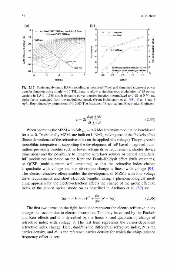
a ¼ 2Id/ðtÞ=dt

dIðtÞ=dtð2:35Þ

When operating the MZM withDUbias = p/4 ideal intensity modulation is achievedfor a = 0. Traditionally MZMs are built on LiNbO3 making use of the Pockels effect(linear dependence of the refractive index on the applied bias voltage). The progress inmonolithic integration is supporting the development of InP-based integrated trans-mitters providing benefits such as lower voltage drive requirements, shorter devicedimensions and the possibility to integrate with laser sources or optical amplifiers.InP modulators are based on the Kerr and Frank–Keldysh effect (bulk structures)or QCSE (multi-quantum well structures) so that the refractive index changeis quadratic with voltage and the absorption change is linear with voltage [94].The electro-refractive effect enables the development of MZMs with low voltagedrive requirements and short electrode lengths. Using a phenomenological mod-eling approach for the electro-refraction affects the change of the group effectiveindex of the guided optical mode Dn as described in Arellano et al. [89] as:

Dn ¼ r1V þ r2V2 þ dn

dNN � N0ð Þ ð2:36Þ

The first two terms on the right-hand side represent the electro-refractive indexchange that occurs due to electro-absorption. This may be caused by the Pockelsand Kerr effects and it is described by the linear r1 and quadratic r2 change ofrefractive index with voltage V. The last term represents the carrier-dependentrefractive index change. Here, dn/dN is the differential refractive index, N is thecarrier density, and N0 is the reference carrier density for which the chirp-inducedfrequency offset is zero.

Fig. 2.17 Static and dynamic EAM modeling. a measured (lines) and simulated (squares) powertransfer function using single *10 THz band to allow a simultaneous modulation of 13 opticalcarriers in 1,540–1,588 nm; b dynamic power transfer function (normalized to 0 dB at 0 V) andalpha factor extracted from the modulated signal. (From Koltchanov et al. [93], Figs. 1 and 3right. Reproduced by permission of � 2005 The Institute of Electrical and Electronics Engineers)

52 A. Richter

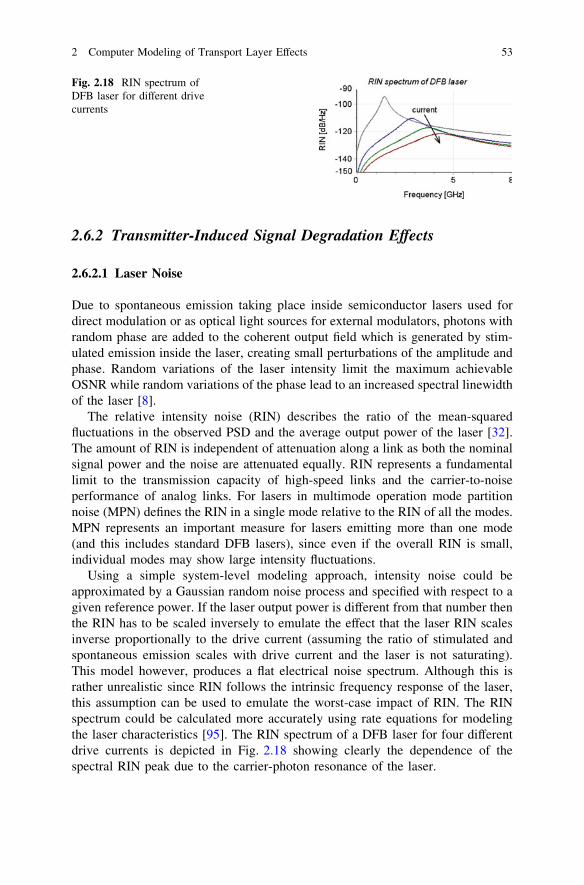
2.6.2 Transmitter-Induced Signal Degradation Effects

2.6.2.1 Laser Noise

Due to spontaneous emission taking place inside semiconductor lasers used fordirect modulation or as optical light sources for external modulators, photons withrandom phase are added to the coherent output field which is generated by stim-ulated emission inside the laser, creating small perturbations of the amplitude andphase. Random variations of the laser intensity limit the maximum achievableOSNR while random variations of the phase lead to an increased spectral linewidthof the laser [8].

The relative intensity noise (RIN) describes the ratio of the mean-squaredfluctuations in the observed PSD and the average output power of the laser [32].The amount of RIN is independent of attenuation along a link as both the nominalsignal power and the noise are attenuated equally. RIN represents a fundamentallimit to the transmission capacity of high-speed links and the carrier-to-noiseperformance of analog links. For lasers in multimode operation mode partitionnoise (MPN) defines the RIN in a single mode relative to the RIN of all the modes.MPN represents an important measure for lasers emitting more than one mode(and this includes standard DFB lasers), since even if the overall RIN is small,individual modes may show large intensity fluctuations.

Using a simple system-level modeling approach, intensity noise could beapproximated by a Gaussian random noise process and specified with respect to agiven reference power. If the laser output power is different from that number thenthe RIN has to be scaled inversely to emulate the effect that the laser RIN scalesinverse proportionally to the drive current (assuming the ratio of stimulated andspontaneous emission scales with drive current and the laser is not saturating).This model however, produces a flat electrical noise spectrum. Although this israther unrealistic since RIN follows the intrinsic frequency response of the laser,this assumption can be used to emulate the worst-case impact of RIN. The RINspectrum could be calculated more accurately using rate equations for modelingthe laser characteristics [95]. The RIN spectrum of a DFB laser for four differentdrive currents is depicted in Fig. 2.18 showing clearly the dependence of thespectral RIN peak due to the carrier-photon resonance of the laser.

Fig. 2.18 RIN spectrum ofDFB laser for different drivecurrents


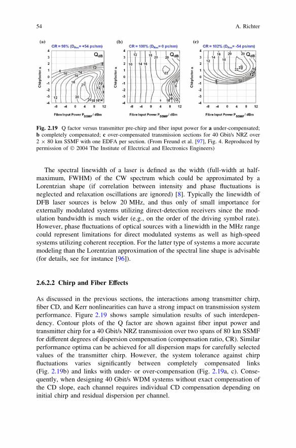
The spectral linewidth of a laser is defined as the width (full-width at half-maximum, FWHM) of the CW spectrum which could be approximated by aLorentzian shape (if correlation between intensity and phase fluctuations isneglected and relaxation oscillations are ignored) [8]. Typically the linewidth ofDFB laser sources is below 20 MHz, and thus only of small importance forexternally modulated systems utilizing direct-detection receivers since the mod-ulation bandwidth is much wider (e.g., on the order of the driving symbol rate).However, phase fluctuations of optical sources with a linewidth in the MHz rangecould represent limitations for direct modulated systems as well as high-speedsystems utilizing coherent reception. For the latter type of systems a more accuratemodeling than the Lorentzian approximation of the spectral line shape is advisable(for details, see for instance [96]).

2.6.2.2 Chirp and Fiber Effects

As discussed in the previous sections, the interactions among transmitter chirp,fiber CD, and Kerr nonlinearities can have a strong impact on transmission systemperformance. Figure 2.19 shows sample simulation results of such interdepen-dency. Contour plots of the Q factor are shown against fiber input power andtransmitter chirp for a 40 Gbit/s NRZ transmission over two spans of 80 km SSMFfor different degrees of dispersion compensation (compensation ratio, CR). Similarperformance optima can be achieved for all dispersion maps for carefully selectedvalues of the transmitter chirp. However, the system tolerance against chirpfluctuations varies significantly between completely compensated links(Fig. 2.19b) and links with under- or over-compensation (Fig. 2.19a, c). Conse-quently, when designing 40 Gbit/s WDM systems without exact compensation ofthe CD slope, each channel requires individual CD compensation depending oninitial chirp and residual dispersion per channel.

Fig. 2.19 Q factor versus transmitter pre-chirp and fiber input power for a under-compensated;b completely compensated; c over-compensated transmission sections for 40 Gbit/s NRZ over2 9 80 km SSMF with one EDFA per section. (From Freund et al. [97], Fig. 4. Reproduced bypermission of � 2004 The Institute of Electrical and Electronics Engineers)

54 A. Richter

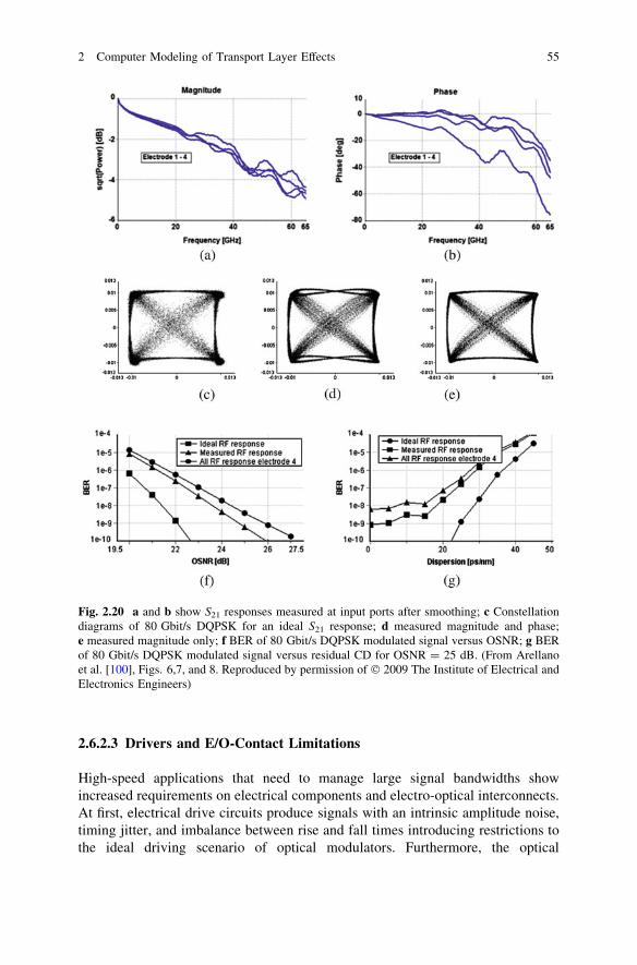
2.6.2.3 Drivers and E/O-Contact Limitations

High-speed applications that need to manage large signal bandwidths showincreased requirements on electrical components and electro-optical interconnects.At first, electrical drive circuits produce signals with an intrinsic amplitude noise,timing jitter, and imbalance between rise and fall times introducing restrictions tothe ideal driving scenario of optical modulators. Furthermore, the optical

Fig. 2.20 a and b show S21 responses measured at input ports after smoothing; c Constellationdiagrams of 80 Gbit/s DQPSK for an ideal S21 response; d measured magnitude and phase;e measured magnitude only; f BER of 80 Gbit/s DQPSK modulated signal versus OSNR; g BERof 80 Gbit/s DQPSK modulated signal versus residual CD for OSNR = 25 dB. (From Arellanoet al. [100], Figs. 6,7, and 8. Reproduced by permission of � 2009 The Institute of Electrical andElectronics Engineers)


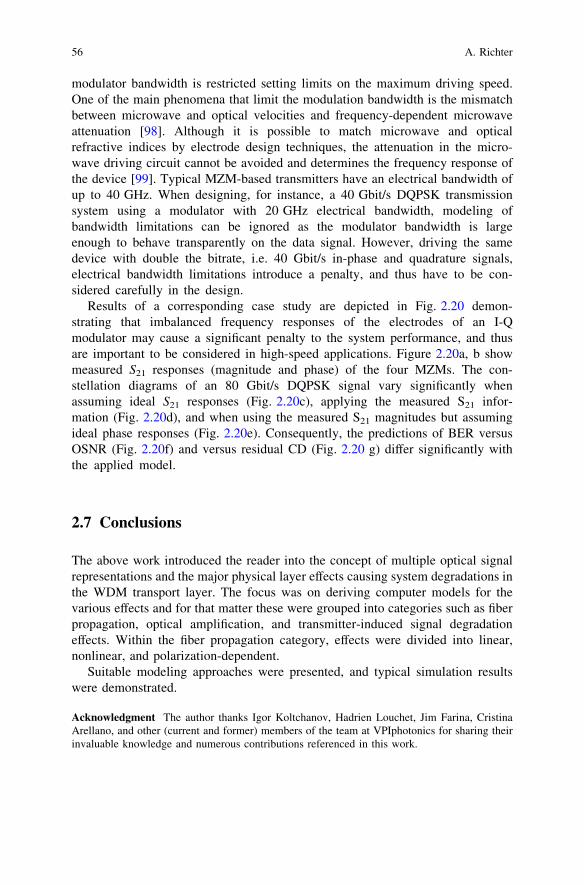
modulator bandwidth is restricted setting limits on the maximum driving speed.One of the main phenomena that limit the modulation bandwidth is the mismatchbetween microwave and optical velocities and frequency-dependent microwaveattenuation [98]. Although it is possible to match microwave and opticalrefractive indices by electrode design techniques, the attenuation in the micro-wave driving circuit cannot be avoided and determines the frequency response ofthe device [99]. Typical MZM-based transmitters have an electrical bandwidth ofup to 40 GHz. When designing, for instance, a 40 Gbit/s DQPSK transmissionsystem using a modulator with 20 GHz electrical bandwidth, modeling ofbandwidth limitations can be ignored as the modulator bandwidth is largeenough to behave transparently on the data signal. However, driving the samedevice with double the bitrate, i.e. 40 Gbit/s in-phase and quadrature signals,electrical bandwidth limitations introduce a penalty, and thus have to be con-sidered carefully in the design.

Results of a corresponding case study are depicted in Fig. 2.20 demon-strating that imbalanced frequency responses of the electrodes of an I-Qmodulator may cause a significant penalty to the system performance, and thusare important to be considered in high-speed applications. Figure 2.20a, b showmeasured S21 responses (magnitude and phase) of the four MZMs. The con-stellation diagrams of an 80 Gbit/s DQPSK signal vary significantly whenassuming ideal S21 responses (Fig. 2.20c), applying the measured S21 infor-mation (Fig. 2.20d), and when using the measured S21 magnitudes but assumingideal phase responses (Fig. 2.20e). Consequently, the predictions of BER versusOSNR (Fig. 2.20f) and versus residual CD (Fig. 2.20 g) differ significantly withthe applied model.

2.7 Conclusions

The above work introduced the reader into the concept of multiple optical signalrepresentations and the major physical layer effects causing system degradations inthe WDM transport layer. The focus was on deriving computer models for thevarious effects and for that matter these were grouped into categories such as fiberpropagation, optical amplification, and transmitter-induced signal degradationeffects. Within the fiber propagation category, effects were divided into linear,nonlinear, and polarization-dependent.

Suitable modeling approaches were presented, and typical simulation resultswere demonstrated.

Acknowledgment The author thanks Igor Koltchanov, Hadrien Louchet, Jim Farina, CristinaArellano, and other (current and former) members of the team at VPIphotonics for sharing theirinvaluable knowledge and numerous contributions referenced in this work.

56 A. Richter

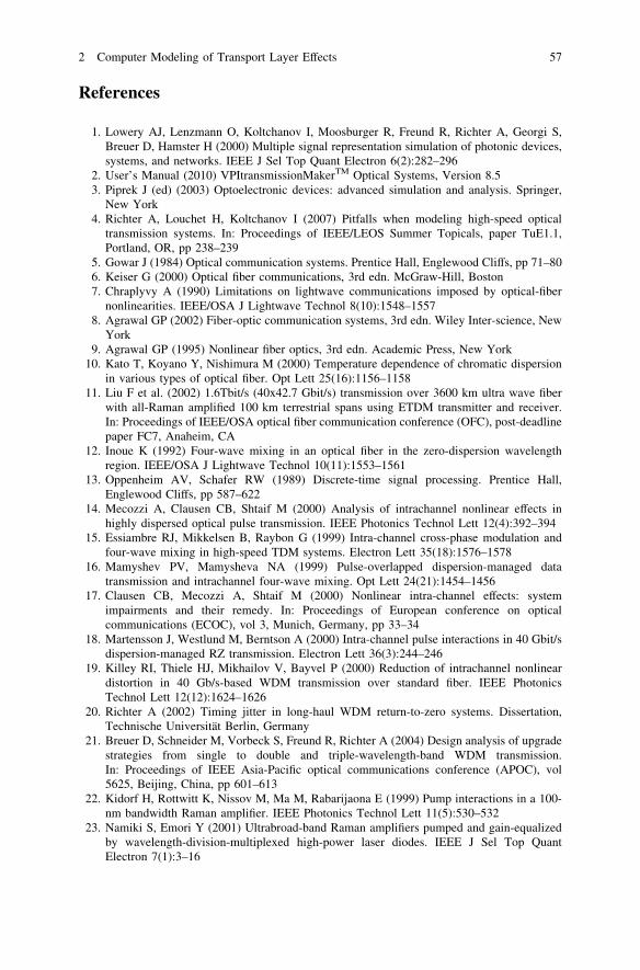
References

1. Lowery AJ, Lenzmann O, Koltchanov I, Moosburger R, Freund R, Richter A, Georgi S,Breuer D, Hamster H (2000) Multiple signal representation simulation of photonic devices,systems, and networks. IEEE J Sel Top Quant Electron 6(2):282–296

2. User’s Manual (2010) VPItransmissionMakerTM Optical Systems, Version 8.53. Piprek J (ed) (2003) Optoelectronic devices: advanced simulation and analysis. Springer,

New York4. Richter A, Louchet H, Koltchanov I (2007) Pitfalls when modeling high-speed optical

transmission systems. In: Proceedings of IEEE/LEOS Summer Topicals, paper TuE1.1,Portland, OR, pp 238–239

5. Gowar J (1984) Optical communication systems. Prentice Hall, Englewood Cliffs, pp 71–806. Keiser G (2000) Optical fiber communications, 3rd edn. McGraw-Hill, Boston7. Chraplyvy A (1990) Limitations on lightwave communications imposed by optical-fiber

nonlinearities. IEEE/OSA J Lightwave Technol 8(10):1548–15578. Agrawal GP (2002) Fiber-optic communication systems, 3rd edn. Wiley Inter-science, New

York9. Agrawal GP (1995) Nonlinear fiber optics, 3rd edn. Academic Press, New York

10. Kato T, Koyano Y, Nishimura M (2000) Temperature dependence of chromatic dispersionin various types of optical fiber. Opt Lett 25(16):1156–1158

11. Liu F et al. (2002) 1.6Tbit/s (40x42.7 Gbit/s) transmission over 3600 km ultra wave fiberwith all-Raman amplified 100 km terrestrial spans using ETDM transmitter and receiver.In: Proceedings of IEEE/OSA optical fiber communication conference (OFC), post-deadlinepaper FC7, Anaheim, CA

12. Inoue K (1992) Four-wave mixing in an optical fiber in the zero-dispersion wavelengthregion. IEEE/OSA J Lightwave Technol 10(11):1553–1561

13. Oppenheim AV, Schafer RW (1989) Discrete-time signal processing. Prentice Hall,Englewood Cliffs, pp 587–622

14. Mecozzi A, Clausen CB, Shtaif M (2000) Analysis of intrachannel nonlinear effects inhighly dispersed optical pulse transmission. IEEE Photonics Technol Lett 12(4):392–394

15. Essiambre RJ, Mikkelsen B, Raybon G (1999) Intra-channel cross-phase modulation andfour-wave mixing in high-speed TDM systems. Electron Lett 35(18):1576–1578

16. Mamyshev PV, Mamysheva NA (1999) Pulse-overlapped dispersion-managed datatransmission and intrachannel four-wave mixing. Opt Lett 24(21):1454–1456

17. Clausen CB, Mecozzi A, Shtaif M (2000) Nonlinear intra-channel effects: systemimpairments and their remedy. In: Proceedings of European conference on opticalcommunications (ECOC), vol 3, Munich, Germany, pp 33–34

18. Martensson J, Westlund M, Berntson A (2000) Intra-channel pulse interactions in 40 Gbit/sdispersion-managed RZ transmission. Electron Lett 36(3):244–246

19. Killey RI, Thiele HJ, Mikhailov V, Bayvel P (2000) Reduction of intrachannel nonlineardistortion in 40 Gb/s-based WDM transmission over standard fiber. IEEE PhotonicsTechnol Lett 12(12):1624–1626

20. Richter A (2002) Timing jitter in long-haul WDM return-to-zero systems. Dissertation,Technische Universität Berlin, Germany

21. Breuer D, Schneider M, Vorbeck S, Freund R, Richter A (2004) Design analysis of upgradestrategies from single to double and triple-wavelength-band WDM transmission.In: Proceedings of IEEE Asia-Pacific optical communications conference (APOC), vol5625, Beijing, China, pp 601–613

22. Kidorf H, Rottwitt K, Nissov M, Ma M, Rabarijaona E (1999) Pump interactions in a 100-nm bandwidth Raman amplifier. IEEE Photonics Technol Lett 11(5):530–532

23. Namiki S, Emori Y (2001) Ultrabroad-band Raman amplifiers pumped and gain-equalizedby wavelength-division-multiplexed high-power laser diodes. IEEE J Sel Top QuantElectron 7(1):3–16


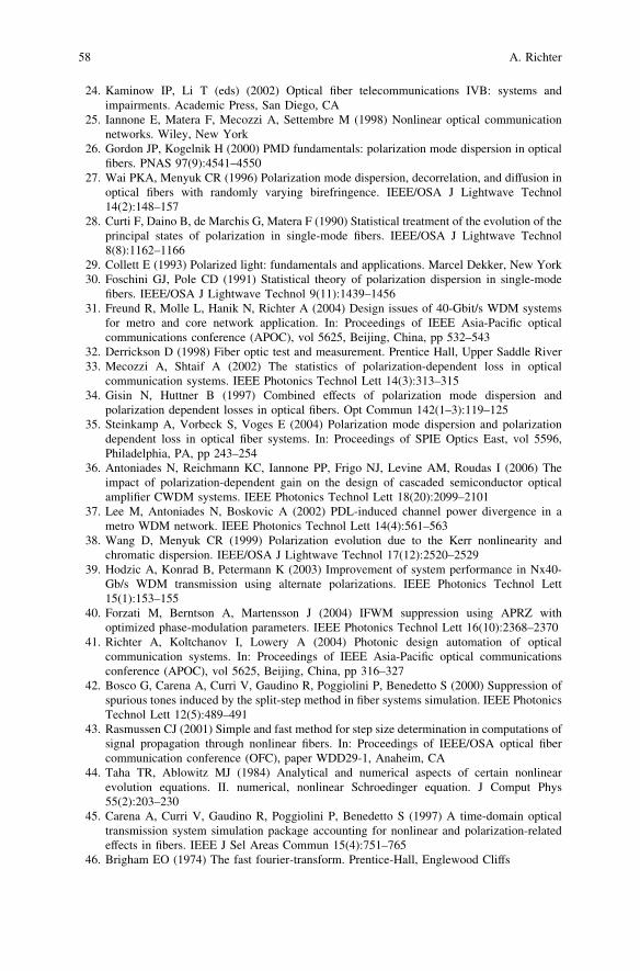
24. Kaminow IP, Li T (eds) (2002) Optical fiber telecommunications IVB: systems andimpairments. Academic Press, San Diego, CA

25. Iannone E, Matera F, Mecozzi A, Settembre M (1998) Nonlinear optical communicationnetworks. Wiley, New York

26. Gordon JP, Kogelnik H (2000) PMD fundamentals: polarization mode dispersion in opticalfibers. PNAS 97(9):4541–4550

27. Wai PKA, Menyuk CR (1996) Polarization mode dispersion, decorrelation, and diffusion inoptical fibers with randomly varying birefringence. IEEE/OSA J Lightwave Technol14(2):148–157

28. Curti F, Daino B, de Marchis G, Matera F (1990) Statistical treatment of the evolution of theprincipal states of polarization in single-mode fibers. IEEE/OSA J Lightwave Technol8(8):1162–1166

29. Collett E (1993) Polarized light: fundamentals and applications. Marcel Dekker, New York30. Foschini GJ, Pole CD (1991) Statistical theory of polarization dispersion in single-mode

fibers. IEEE/OSA J Lightwave Technol 9(11):1439–145631. Freund R, Molle L, Hanik N, Richter A (2004) Design issues of 40-Gbit/s WDM systems

for metro and core network application. In: Proceedings of IEEE Asia-Pacific opticalcommunications conference (APOC), vol 5625, Beijing, China, pp 532–543

32. Derrickson D (1998) Fiber optic test and measurement. Prentice Hall, Upper Saddle River33. Mecozzi A, Shtaif A (2002) The statistics of polarization-dependent loss in optical

communication systems. IEEE Photonics Technol Lett 14(3):313–31534. Gisin N, Huttner B (1997) Combined effects of polarization mode dispersion and

polarization dependent losses in optical fibers. Opt Commun 142(1–3):119–12535. Steinkamp A, Vorbeck S, Voges E (2004) Polarization mode dispersion and polarization

dependent loss in optical fiber systems. In: Proceedings of SPIE Optics East, vol 5596,Philadelphia, PA, pp 243–254

36. Antoniades N, Reichmann KC, Iannone PP, Frigo NJ, Levine AM, Roudas I (2006) Theimpact of polarization-dependent gain on the design of cascaded semiconductor opticalamplifier CWDM systems. IEEE Photonics Technol Lett 18(20):2099–2101

37. Lee M, Antoniades N, Boskovic A (2002) PDL-induced channel power divergence in ametro WDM network. IEEE Photonics Technol Lett 14(4):561–563

38. Wang D, Menyuk CR (1999) Polarization evolution due to the Kerr nonlinearity andchromatic dispersion. IEEE/OSA J Lightwave Technol 17(12):2520–2529

39. Hodzic A, Konrad B, Petermann K (2003) Improvement of system performance in Nx40-Gb/s WDM transmission using alternate polarizations. IEEE Photonics Technol Lett15(1):153–155

40. Forzati M, Berntson A, Martensson J (2004) IFWM suppression using APRZ withoptimized phase-modulation parameters. IEEE Photonics Technol Lett 16(10):2368–2370

41. Richter A, Koltchanov I, Lowery A (2004) Photonic design automation of opticalcommunication systems. In: Proceedings of IEEE Asia-Pacific optical communicationsconference (APOC), vol 5625, Beijing, China, pp 316–327

42. Bosco G, Carena A, Curri V, Gaudino R, Poggiolini P, Benedetto S (2000) Suppression ofspurious tones induced by the split-step method in fiber systems simulation. IEEE PhotonicsTechnol Lett 12(5):489–491

43. Rasmussen CJ (2001) Simple and fast method for step size determination in computations ofsignal propagation through nonlinear fibers. In: Proceedings of IEEE/OSA optical fibercommunication conference (OFC), paper WDD29-1, Anaheim, CA

44. Taha TR, Ablowitz MJ (1984) Analytical and numerical aspects of certain nonlinearevolution equations. II. numerical, nonlinear Schroedinger equation. J Comput Phys55(2):203–230

45. Carena A, Curri V, Gaudino R, Poggiolini P, Benedetto S (1997) A time-domain opticaltransmission system simulation package accounting for nonlinear and polarization-relatedeffects in fibers. IEEE J Sel Areas Commun 15(4):751–765

46. Brigham EO (1974) The fast fourier-transform. Prentice-Hall, Englewood Cliffs

58 A. Richter

47. Singleton RC (1967) A method for computing the fast Fourier transform with auxiliarymemory and limited high-speed storage. IEEE Trans Audio Electroacoustics 15(2):91–98

48. Yu T, Reimer WM, Grigoryan VS, Menyuk CR (2000) A mean field approach forsimulating wavelength-division multiplexed systems. IEEE Photonics Technol Lett12(4):443–445

49. Wai PKA, Menyuk CR, Chen HH (1991) Stability of solitons in randomly varyingbirefringent fibers. Opt Lett 16(16):1231–1233

50. Marcuse D, Menyuk CR, Wai PKA (1997) Application of the Manakov-PMD equation tostudies of signal propagation in optical fibers with randomly varying birefringence. IEEE/OSA J Lightwave Technol 15(9):1735–1746

51. Biondini G, Kath WL, Menyuk CR (2002) Importance sampling for polarization-modedispersion. IEEE Photonics Technol Lett 14(3):310–312

52. Menyuk CR (1987) Nonlinear pulse propagation in birefringence optical fibers. IEEE JQuant Electron 23(2):174–176

53. Nelson LE, Jopson R (2002) Introduction to polarization mode dispersion in lightwavesystems Venice Summer School on PMD, Venice, Italy, pp 24–26

54. Shtaif M, Mecozzi A (2000) Study of the frequency autocorrelation of the differential groupdelay in fibers with polarization mode dispersion. Opt Lett 25(10):707–709

55. Richter A, Dazert M, Koltchanov I, Myslivets E, Lowery A (2002) Performancedegradations in high-speed (40 Gbit/s +) transmission systems due to polarization modedispersion. In: Proceedings of IEEE/OSA national fiber optics engineers conference(NFOEC), paper 073, Anaheim, CA

56. Richter A, Koltchanov I, Kuzmin K, Myslivets E, Freund R (2005) Issues on bit-error rateestimation for fiber-optic communication systems. In: Proceedings of IEEE/OSA opticalfiber communication conference (OFC/NFOEC), paper NTuH3, Anaheim, CA

57. Richter A, Koltchanov I, Kuzmin K, Rukhlenko D (2005) Bit-error rate estimation forapplications using 40 Gbit/s and higher. In: Proceedings of IEEE workshop on opticaltransmission and equalization (WOTE), paper B3, Shanghai, China, pp 23–24

58. Francia C, Bruyere F, Penninckx D, Chbat M (1998) PMD second-order effects on pulsepropagation in single-mode optical fibers. IEEE Photonics Technol Lett 10(12):1739–1741

59. Kogelnik H, Nelson LE, Gordon JP, Jopson RM (2000) Jones matrix for second-orderpolarization mode dispersion. Opt Lett 25(1):19–21

60. Eyal A, Marshall WK, Tur M, Yariv A (1999) Representation of second-order polarizationmode dispersion. IEEE Electron Lett 35(19):1658–1659

61. Orlandini A, Vincetti L (2001) A simple and useful model for Jones matrix to evaluatehigher order polarization-mode dispersion effects. IEEE Photonics Technol Lett13(11):1176–1178

62. Poloyko I, Khilo A, Myslivets E, Volkov V, Koltchanov I, Richter A, Lowery A (2003)Photonic design automation of Raman amplified systems. In: Proceedings of IEEE/OSAnational fiber optics engineers conference (NFOEC), paper P29, Atlanta, GA

63. Photonic Modules Reference Manual (2011) VPItransmissionMaker TMOptical Systems,Version 8.6

64. Rottwitt K, Bromage J, Leng L (2002) Scaling the Raman gain coefficient of optical fibers.In: Proceedings of European conference on optical communications (ECOC), paper S3.03,Copenhagen, Denmark

65. Grant AR (2002) Calculating the Raman pump distribution to achieve minimum gain ripple.IEEE J Quant Electron 38(11):1503–1509

66. Perlin VE, Wintful HG (2002) On distributed Raman amplification for ultrabroad-bandlong-haul WDM systems. IEEE/OSA J Lightwave Technol 20(3):409–416

67. Richter A, Koltchanov I, Myslivets E, Khilo A, Shkred G, Freund R (2005) Optimization ofmulti-pump Raman amplifiers. In: Proceedings of IEEE/OSA optical fiber communicationconference (OFC/NFOEC), paper NTuB4, Anaheim, CA

68. Lin Q, Agrawal G (2003) PMD effects in fiber-based Raman amplifiers. In: Proceedings ofIEEE/OSA optical fiber communication conference (OFC), paper TuC4, Atlanta, GA


69. Richter A, Louchet H, Poloyko I, Karelin N, Farina J, Koltchanov I (2009) A parametricapproach to optical systems design, optimization and validation. In: Proceedings ofEuropean conference on networks and optical communications (NOC), Valladolid, Spain,pp 361–367

70. Mears RJ, Reekie L, Jauncey IM, Payne DN (1987) Low noise erbium doped fiber amplifieroperating at 1.54 lm. IEEE Electron Lett 23(19):1026–1028

71. Desurvire E (1994) Erbium-doped fiber amplifiers, principles and applications. Wiley, NewYork

72. Becker PC, Olsson NA, Simpson JR (1999) Erbium-doped fiber amplifiers, fundamentalsand technology. Academic Press, New York

73. Giles R, Desurvire E (1991) Modeling erbium-doped fiber amplifiers. IEEE/OSA JLightwave Technol 9(2):271–283

74. User’s Manual (2011) VPIcomponentMaker TMOptical Amplifiers, Version 8.675. Abramovich F, Bayvel P (1997) Some statistical remarks on the derivation of BER in

amplified optical communication systems. IEEE Trans Commun 45(9):1032–103476. Keiser G (2000) Optical fiber communications, 3rd edn. McGraw-Hill, Boston77. Collin RE (1992) Foundations for microwave engineering, 2nd edn. McGraw-Hill, New

York78. Bonnedal D (1996) EDFA gain described with a black box model. In: Proceedings of OSA

trends in optics and photonics, optical amplifiers and their applications, vol 5, Washington,D.C., pp 53–56

79. Burgmeier J, Cords A, März R, Schäffer C, Stummer B (1998) A black box model ofEDFA’s operating in WDM systems. IEEE/OSA J Lightwave Technol 16(7):1271–1275

80. Zhang X, Mitchell A (2000) A simple black box model for erbium-doped fiber amplifiers.IEEE Photonics Technol Lett 12(1):28–30

81. Jacobsen G, Persson U, Gillner L, Vanin E, Wingstrand S (2000) Pump power dependentblack box EDFA model. J Opt Commun 21(5):171–177

82. Villa JAL, Bo FB, Querol VP, Teixeira AL, Prat Goma J (2008) Extended black box modelfor fiber length variation of erbium-doped fiber amplifiers. IEEE Photonics Technol Lett20(24):2063–2065

83. Richter A, Devatine R, Koltchanov I, Lowery A, Khomchenko D, Yevseyenko D, Moar P(2002) Virtual product prototyping of erbium doped fiber amplifiers for applications indense WDM systems. In: Proceedings of IEEE/OSA national fiber optics engineersconference (NFOEC), paper 153, Anaheim, CA

84. Yoo SJB, Xin W, Garratt LD, Young JC, Ellinas G, Chiao JC, Rauch M, Baran JE, MeagherB, Leblanc H, Chang G-K (1998) Observation of prolonged power transients in areconfigurable multiwavelength network and their suppression by gain-clamping of opticalamplifiers. IEEE Photonics Technol Lett 10(11):1659–1661

85. Richter A, Karelin N, Louchet H, Koltchanov I, Farina J (2010) Dynamic events in opticalnetworks—emulation and performance impact analysis. In: Proceedings of IEEE militarycommunication conference (MILCOM), San Jose, CA, pp 1083–1087

86. Matsui Y, Mahgerefteh D, Zheng X, Liao C, Fan ZF, McCallion K, Tayebati P (2006)Chirp-managed directly modulated laser (CML). IEEE Photonics Technol Lett 18(2):385–387

87. Cartledge JC, Srinivasan RC (1997) Extraction of DFB laser rate equation parameters forsystem simulation purposes. IEEE/OSA J Lightwave Technol 15(5):852–860

88. Lowery AJ (1992) A two-port bilateral model for semiconductor lasers. IEEE J QuantElectron 28(1):82–92

89. Arellano C, Mingaleev S, Novitsky A, Koltchanov I, Richter A (2009) Design of complexsemiconductor integrated structures. In: Proceedings of IEEE Asia communication andphoton conference (ACP) 7631, paper 7631-106, Shanghai, China

90. Gnauck AH, Korotky SK, Veselka J, Nagal J, Kemmener CT, Mindford WJ, Moser DT(1991) Dispersion penalty reduction using an optical modulator with adjustable chirp. IEEEPhotonics Technol Lett 3(10):916–918

60 A. Richter

91. Hashimoto JI, Nakano Y, Tada K (1992) Influence of facet reflection on the performance ofa DFB laser integrated with an optical amplifier/modulator. IEEE J Quant Electron28(3):594–603

92. Koyama F, Iga K (1998) Frequency chirping in external modulators. IEEE/OSA JLightwave Technol 6(1):87–93

93. Koltchanov I, Richter A, Myslivets E, Kazmierski C (2005) Complete time and frequency-dependent modeling of electro-absorption modulators. In: Proceedings of IEEE/OSA opticalfiber communication conference (OFC/NFOEC), paper OME42, Anaheim, CA

94. Mendoza-Alvarez JG, Coldren LA, Alping A, Yan RH, Hausken T, Lee K, Pedrottin K(1988) Analysis of depletion edge translation lightwave modulators. IEEE/OSA JLightwave Technol 6(6):793–808

95. Ahmed M, Yamada M, Saito M (2001) Numerical modeling of intensity and phase noise insemiconductor lasers. IEEE J Quant Electron 37(12):1600–1610

96. Betti S, De Marchis G, Iannone E (1995) Coherent optical communication systems. WileyInter-science, New York

97. Freund R, Molle L, Hanik N, Richter A (2004) Design issues of 40 Gbit/s WDM-systemsfor metro and core network application. In: Proceedings of European conference on opticalcommunications (ECOC), paper Tu351, Stockholm, Sweden

98. Kaminow IP, Koch TL (eds) (1997) Optical fiber telecommunications IIIB. Academic Press,San Diego, CA

99. Dutta AK, Dutta NK, Fujiwara M (eds) (2002) WDM technologies: active opticalcomponents. Academic Press, New York

100. Arellano C, Louchet H, Koltchanov I, Richter A (2009) Important device limitations oftransmitter and receiver concepts when designing 100 G transmission systems. In:Proceedings of IEEE international conference on transparent optical networks (ICTON),paper Tu.C2.3, Azores, Portugal


Documents

Chapter 2 Computer Modeling of Transport Layer Effects