Embed Size (px)
Citation preview
11/20/1316/03/2021 Jinniu Hu
Chapter 2Bohr's Model of the Hydrogen
1
Atomic Physics
16/03/2021 Jinniu Hu
The Classical Atomic Model
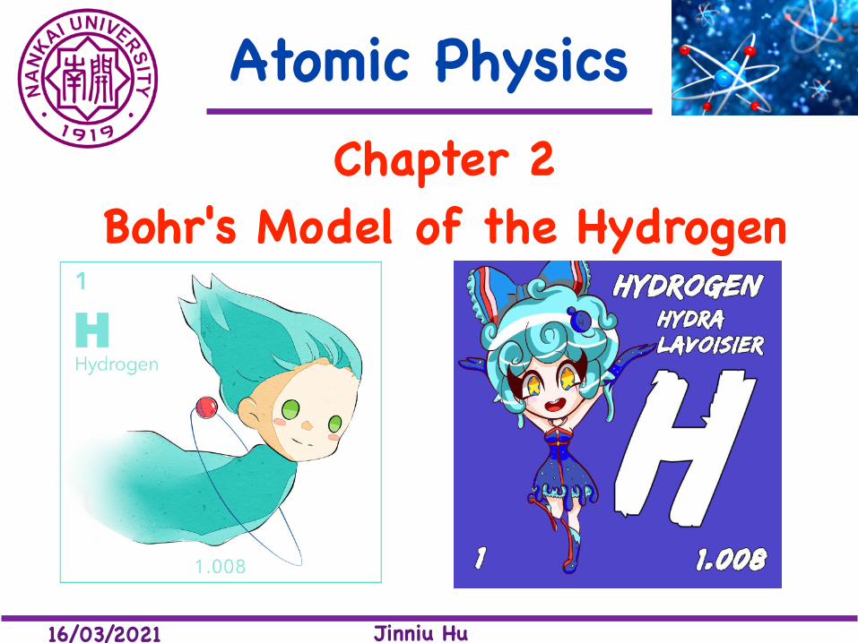
The force of attraction on the electron due to the nucleus is ~F =
�e2
4⇡"0
~r
r3
The electron’s radial acceleration
ar =v2
rwhere v is the tangential velocity of the electron and Newton’s second law now gives
e2
4⇡"0
1
r2=
mv2
rand
v =ep
4⇡"mr
16/03/2021 Jinniu Hu
The Classical Atomic Model
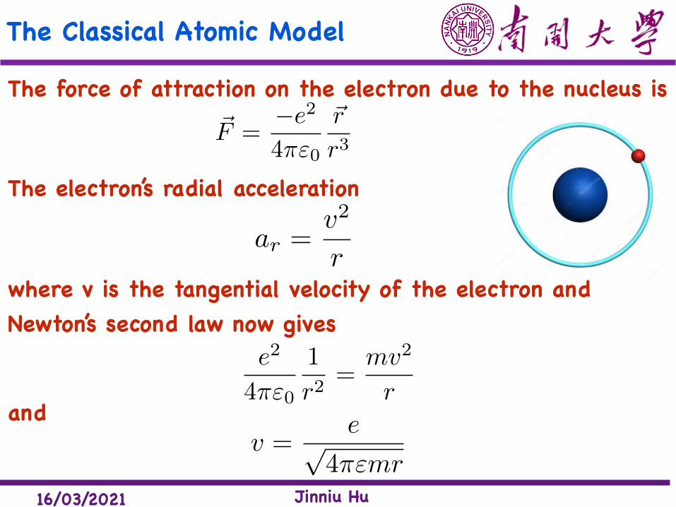
The total mechanical energy is
E =1
2mv2 � e2
4⇡"0rwith the equation about v, we have
E =e2
8⇡"0r� e2
4⇡"0r=
�e2
8⇡"0rThe total energy is negative, indicating a bound system.
An accelerated electric charge continuously radiates energy in the form of electromagnetic radiation!
4.4 The Bohr Model of the Hydrogen Atom 141
Thus far, the classical atomic model seems plausible. The problem arises when we consider that the electron is accelerating due to its circular motion about the nucleus. We know from classical electromagnetic theory that an ac-celerated electric charge continuously radiates energy in the form of electromag-netic radiation. If the electron is radiating energy, then the total energy E of the system, Equation (4.21), must decrease continuously. In order for this to hap-pen, the radius r must decrease. The electron will continuously radiate energy as the electron orbit becomes smaller and smaller until the electron crashes into the nucleus! This process, displayed in Figure 4.14, would occur in about 10!9 s (see Problem 18).
Thus the classical theories of Newton and Maxwell, which had served Rutherford so well in his analysis of a-particle scattering and had thereby en-abled him to discover the nucleus, also led to the failure of the planetary model of the atom. Physics had reached a decisive turning point like that encountered in 1900 with Planck’s revolutionary hypothesis of the quantum behavior of radia-tion. In the early 1910s, however, the answer would not be long in coming, as we shall see in the next section.
4.4 The Bohr Modelof the Hydrogen Atom
Shortly after receiving his Ph.D. from the University of Copenhagen in 1911, the 26-year-old Danish physicist Niels Bohr traveled to Cambridge University to work with J. J. Thomson. He subsequently went to the University of Manchester to work with Rutherford for a few months in 1912 where he became particularly involved in the mysteries of the new Rutherford model of the atom. Bohr returned to the University of Copenhagen in the summer of 1912 with many questions about atomic structure. Like several others, he believed that a fundamental length about the size of an atom (10!10 m) was needed for an atomic model. This funda-mental length might somehow be connected to Planck’s new constant h. The pieces finally came together during the fall and winter of 1912-1913 when Bohr learned of new precise measurements of the hydrogen spectrum and of the em-pirical formulas describing them. He set out to find a fundamental basis from which to derive the Balmer formula [Equation (3.12)], the Ryd berg equation [Equation (3.13)], and Ritz’s combination principles (see Problem 19).
Bohr was well acquainted with Planck’s work on the quantum nature of ra-diation. Like Einstein, Bohr believed that quantum principles should govern more phenomena than just the blackbody spectrum. He was impressed by Einstein’s application of the quantum theory to the photoelectric effect and to the specific heat of solids (see Chapter 9 for the latter) and wondered how the quantum theory might affect atomic structure.
In 1913, following several discussions with Rutherford during 1912 and 1913, Bohr published the paper* “On the Constitution of Atoms and Mole-cules.” He subsequently published several other papers refining and restating his “assumptions” and their predicted results. We will generally follow Bohr’s papers in our discussion.
Planetary model is doomed.
Electron
Nucleus"e
Figure 4.14 The electromag-netic radiation of an orbiting electron in the planetary model of the atom will cause the elec-tron to spiral inward until it crashes into the nucleus.
*Niels Bohr, Philosophical Magazine 26, 1 (1913) and 30, 394 (1915).
03721_ch04_127-161.indd 14103721_ch04_127-161.indd 141 9/29/11 9:36 AM9/29/11 9:36 AM
10�9 s
16/03/2021 Jinniu Hu
Bohr’s general assumptions
A. Certain “stationary states” exist in atoms, which differ from the classical stable states in that the orbiting electrons do not continuously radiate electromagnetic energy. The stationary states are states of definite total energy.
B. The emission or absorption of electromagnetic radiation can occur only in conjunction with a transition between two stationary states. The frequency of the emitted or absorbed radiation is proportional to the difference in energy of the two stationary states (1 and 2): where h is Planck’s constant.
E = E1 � E2 = h⌫
16/03/2021 Jinniu Hu
Bohr’s general assumptions
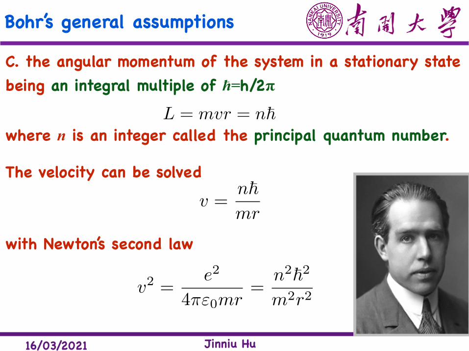
C. the angular momentum of the system in a stationary state being an integral multiple of ħ=h/2!
L = mvr = n~where n is an integer called the principal quantum number.
The velocity can be solved
v =n~mr
with Newton’s second law
v2 =e2
4⇡"0mr=
n2~2m2r2
16/03/2021 Jinniu Hu
Bohr model
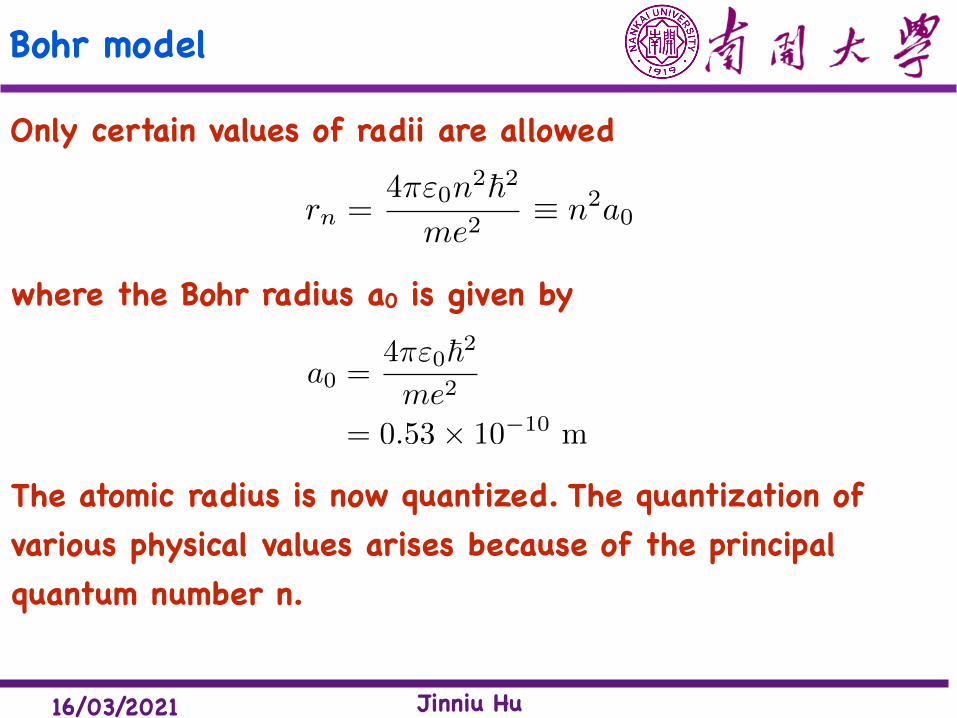
Only certain values of radii are allowed
The atomic radius is now quantized. The quantization of various physical values arises because of the principal quantum number n.
rn =4⇡"0n2~2
me2⌘ n2a0
where the Bohr radius a0 is given by
a0 =4⇡"0~2me2
= 0.53⇥ 10�10 m
16/03/2021 Jinniu Hu
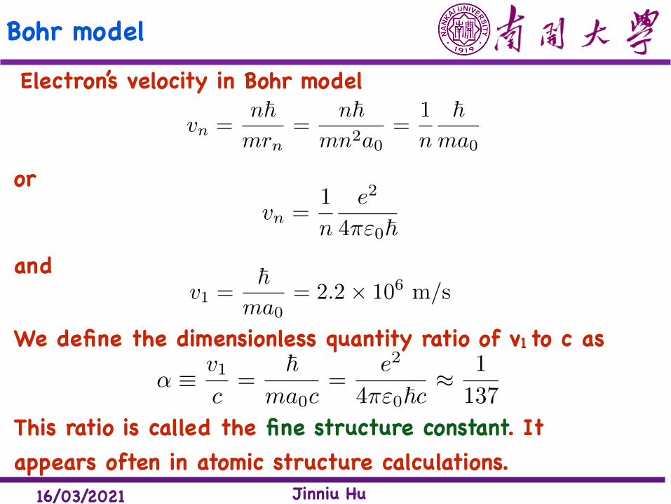
Bohr modelElectron’s velocity in Bohr model
vn =n~mrn
=n~
mn2a0=
1
n
~ma0
orvn =
1
n
e2
4⇡"0~and
v1 =~
ma0= 2.2⇥ 106 m/s
We define the dimensionless quantity ratio of v1 to c as
↵ ⌘ v1c
=~
ma0c=
e2
4⇡"0~c⇡ 1
137
This ratio is called the fine structure constant. It appears often in atomic structure calculations.
16/03/2021 Jinniu Hu
Bohr model
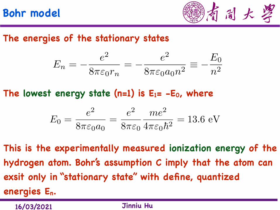
The energies of the stationary states
This is the experimentally measured ionization energy of the hydrogen atom. Bohr’s assumption C imply that the atom can exsit only in “stationary state” with define, quantized energies En.
The lowest energy state (n=1) is E1= -E0, where
En = � e2
8⇡"0rn= � e2
8⇡"0a0n2⌘ �E0
n2
E0 =e2
8⇡"0a0=
e2
8⇡"0
me2
4⇡"0~2= 13.6 eV
16/03/2021 Jinniu Hu
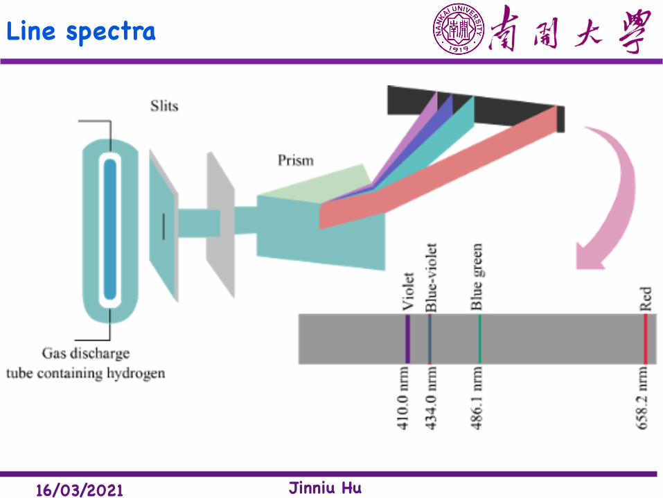
Line spectra
16/03/2021 Jinniu Hu
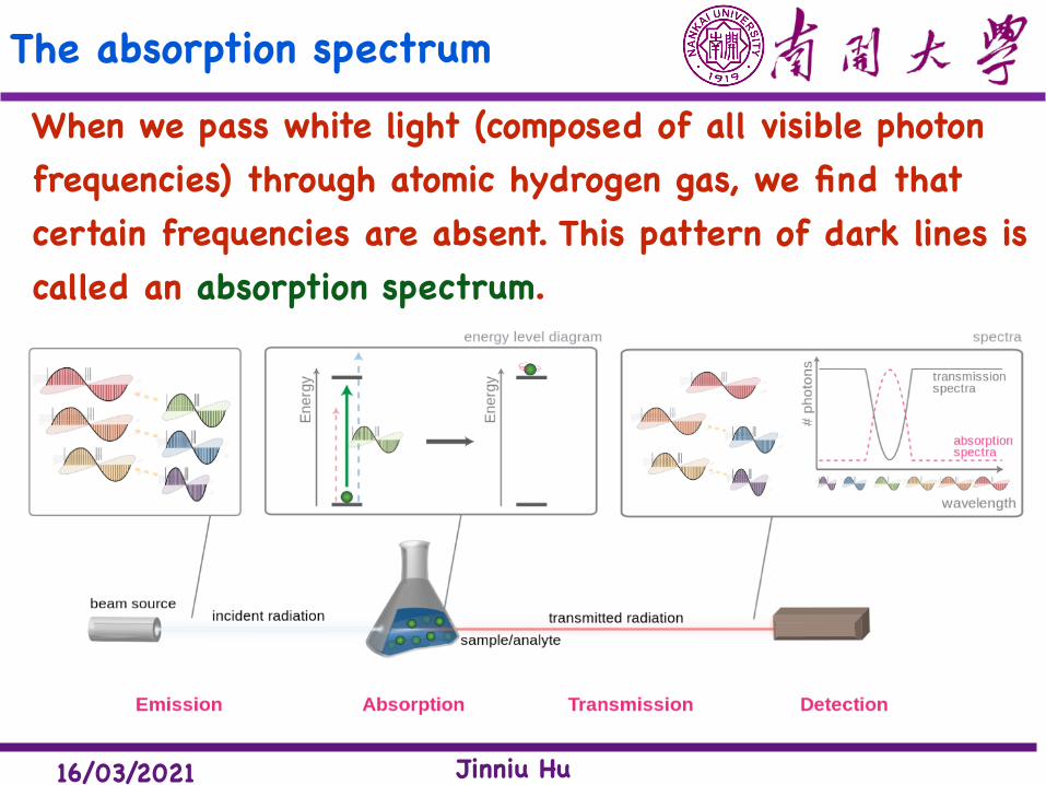
The absorption spectrum When we pass white light (composed of all visible photon frequencies) through atomic hydrogen gas, we find that certain frequencies are absent. This pattern of dark lines is called an absorption spectrum.
16/03/2021 Jinniu Hu
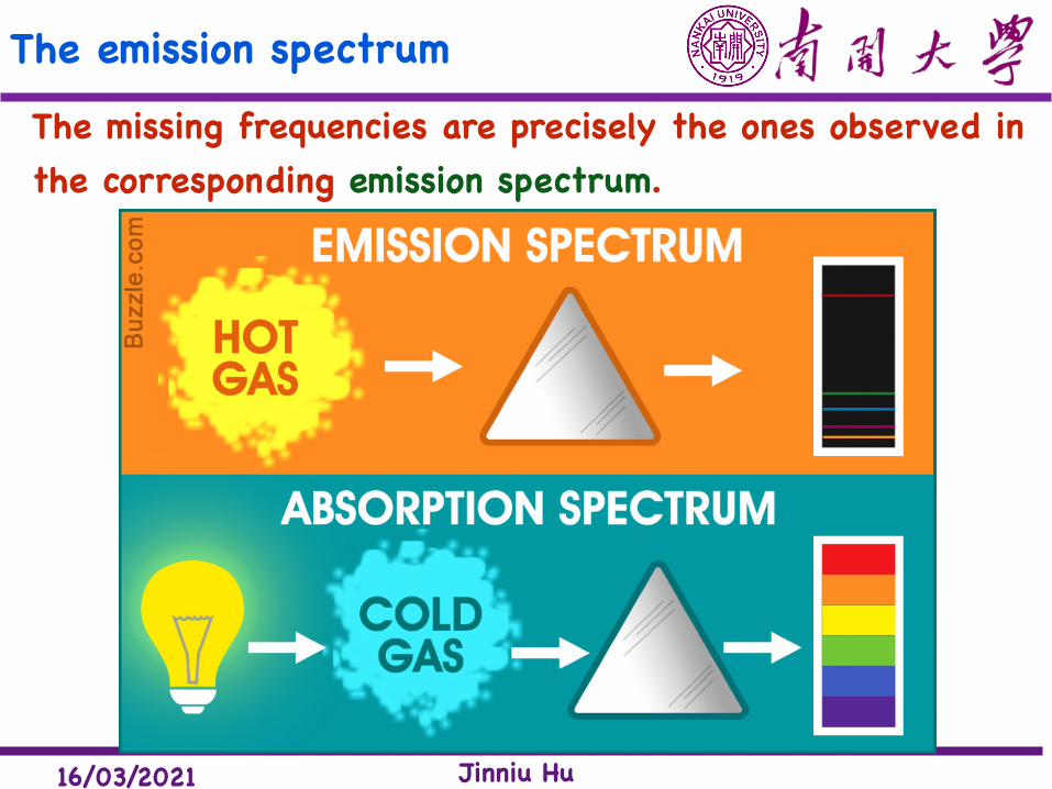
The emission spectrum The missing frequencies are precisely the ones observed in the corresponding emission spectrum.
16/03/2021 Jinniu Hu
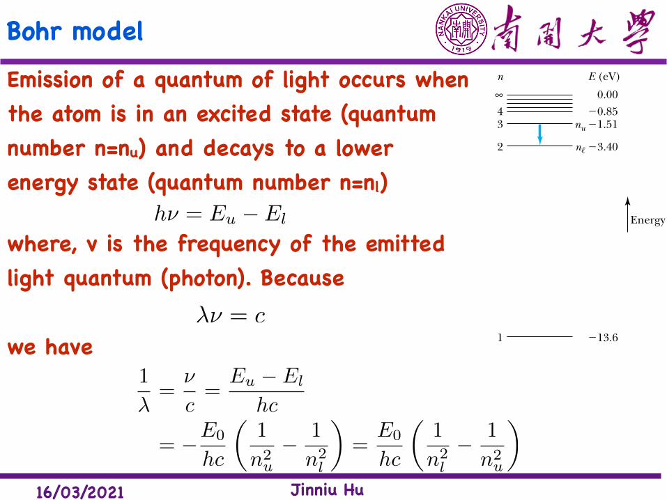
Bohr modelEmission of a quantum of light occurs when the atom is in an excited state (quantum number n=nu) and decays to a lower energy state (quantum number n=nl)
144 Chapter 4 Structure of the Atom
state (n ! n/). A transition between two energy levels is schematically illustrated in Figure 4.15. According to Assumption B we have
hf ! Eu " E/ (4.27)
where f is the frequency of the emitted light quantum (photon). Because lf ! c, we have
1l
!fc !
Eu " E/
hc
!"E0
hca 1
nu2 "
1n /
2 b !E0
hca 1
n /2 "
1nu
2 b (4.28)
where
E0
hc!
me 4
4pc U314pP0 22 ! Rq (4.29)
This constant R q is called the Rydberg constant (for an infinite nuclear mass). Equation (4.28) becomes
1l
! Rq a 1n /
2 "1
nu2 b (4.30)
which is similar to the Rydberg equation (3.13). The value of R q ! 1.097373 # 107 m"1 calculated from Equation (4.29) agrees well with the experimental val-ues given in Chapter 3, and we will obtain an even more accurate result in the next section.
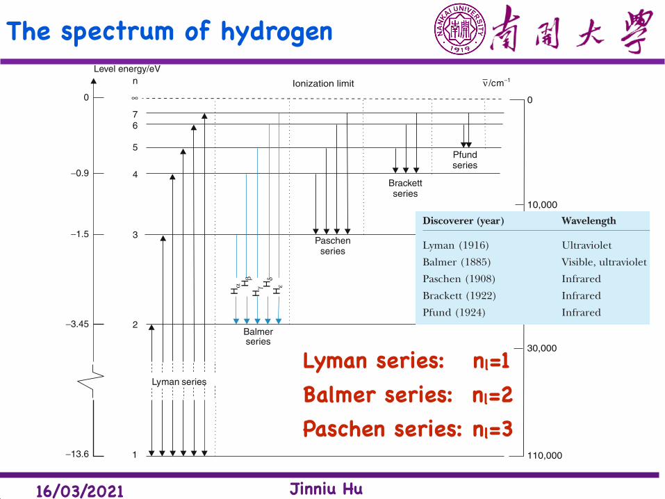
Bohr’s model predicts the frequencies (and wavelengths) of all possible transitions in atomic hydrogen. Several of the series are shown in Figure 4.16. The Lyman series represents transitions to the lowest state with n/ ! 1; the Balmer series results from downward transitions to the stationary state n/ ! 2; and the Paschen series represents transitions to n/ ! 3. As mentioned in Sec-tion 3.3, not all of these series were known experimentally in 1913, but it was clear that Bohr had successfully accounted for the known spectral lines of hydrogen.
The frequencies of the photons in the emission spectrum of an element are directly proportional to the differences in energy of the stationary states. When we pass white light (composed of all visible photon frequencies) through atomic hydrogen gas, we find that certain frequencies are absent. This pattern of dark lines is called an absorption spectrum. The missing frequencies are precisely the ones observed in the corresponding emission spectrum. In absorption, certain photons of light are absorbed, giving up energy to the atom and enabling the electron to move from a lower (/) to a higher (u) stationary state. Equations (4.27) and (4.30) describe the frequencies and wavelengths of the absorbed photons. The atom will remain in the excited state for only a short time (on the order of 10"10 s) before emitting a photon and returning to a lower stationary state. Thus, at ordinary temperatures practically all hydrogen atoms exist in the lowest possible energy state, n ! 1, and only the absorption spectral lines of the Lyman series are normally observed. However, these lines are not in the visible region. The sun produces electromagnetic radiation over a wide range of wave-lengths, including the visible region. When sunlight passes through the sun’s
Bohr predicted new hydrogen wavelengths
Absorption and emission spectrum
Energy
E (eV)
0.00"0.85"1.51
"3.40
n
∞43
2
"13.61
nu
n!
Figure 4.15 The energy-level di-agram of the hydrogen atom. The principal quantum numbers n are shown on the left, with the energy of each level indicated on the right. The ground-state energy is "13.6 eV; negative total energy indicates a bound, attractive system. When an atom is in an excited state (for example, nu ! 3) and decays to a lower stationary state (for exam-ple, n/ ! 2), the hydrogen atom must emit the energy difference in the form of electromagnetic radia-tion; that is, a photon emerges.
03721_ch04_127-161.indd 14403721_ch04_127-161.indd 144 9/29/11 9:36 AM9/29/11 9:36 AM
h⌫ = Eu � El
where, v is the frequency of the emitted light quantum (photon). Because
�⌫ = cwe have
1
�=
⌫
c=
Eu � El
hc
= �E0
hc
✓1
n2u
� 1
n2l
◆=
E0
hc
✓1
n2l
� 1
n2u
◆
16/03/2021 Jinniu Hu
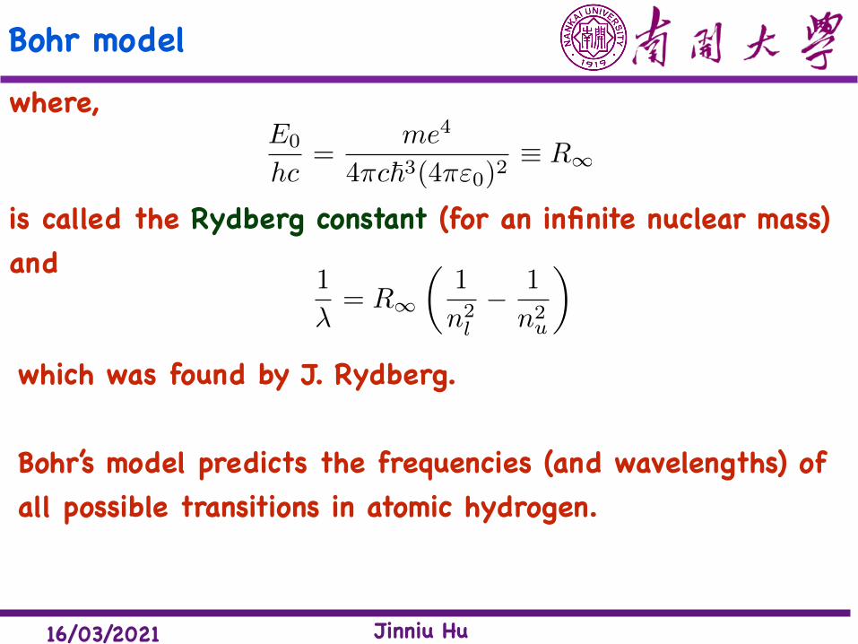
Bohr modelwhere,
E0
hc=
me4
4⇡c~3(4⇡"0)2⌘ R1
is called the Rydberg constant (for an infinite nuclear mass) and
1
�= R1
✓1
n2l
� 1
n2u
◆
which was found by J. Rydberg.
Bohr’s model predicts the frequencies (and wavelengths) of all possible transitions in atomic hydrogen.
106 3 Development of Quantum Physics
Fig. 3.41 Simplified levelscheme of the hydrogen atom andthe different absorption oremission series labelfig
Fig. 3.42 Niels Bohr (1885–1962) From E. Bagge: Die Nobel-preisträger (Heinz-Moos-Verlag, München 1964)
of the circular path of the electron. As long as there are nofurther restrictions for the kinetic energy (µ/2)v2 any radiusr is possible, according to (3.81).
If, however, the electron is described by its matter wavewith wavelength λdB = h/(µv) a stationary state of theatom must be described by a standing wave along the cir-
cle (Fig. 3.43) since the electron should not leave the atom.This gives the quantum condition:
2πr = nλdB (n = 1, 2, 3, . . .), (3.82)
which restricts the possible radii r to the discrete values (3.82).With the de Broglie wavelength λdB = h/(µv) the relation
v = hλ · µ = n
h2πµr
(3.83)
between velocity and radius is obtained. Inserting this into(3.81) yields the possible radii for the electron circles:
rn = n2h2ε0πµZe2
= n2
Za0, (3.84)
where
a0 =ε0h2
πµe2= 5.2917 × 10⁻¹¹ m ≈ 0.5Å
is the smallest radius of the electron (n = 1) in thehydrogen atom (Z = 1), which is named the Bohrradius.
16/03/2021 Jinniu Hu
The spectrum of hydrogen
Lyman series: nl=1Balmer series: nl=2Paschen series: nl=3
94 Chapter 3 The Experimental Basis of Quantum Physics
It is more convenient to take the reciprocal of Equation (3.11) and write Balmer’s formula in the form
1l
!1
364.56 nm k
2 " 4k
2 !4
364.56 nm a 1
22 "1k
2 b ! RH a 122 "
1k
2 b (3.12)
where RH is called the Rydberg constant (for hydrogen) and has the more accurate value 1.096776 # 107 m"1, and k is an integer greater than two (k $ 2).
By 1890, efforts by Johannes Rydberg and particularly Walther Ritz resulted in a more general empirical equation for calculating the wavelengths, called the Ryd berg equation.
1l
! RH a 1n2 "
1k
2 b (3.13)
where n ! 2 corresponds to the Balmer series and k $ n always. In the next 20 years after Balmer’s contribution, other series of the hydrogen atom’s spectral lines were discovered, and by 1925 five series had been discovered, each having a different integer n (Table 3.2). The understanding of the Rydberg equa-tion (3.13) and the discrete spectrum of hydrogen were important research top-ics early in the twentieth century.
Rydberg equation
The visible lines of the Balmer series were observed first because they are most easily seen. Show that the wavelengths of spectral lines in the Lyman (n ! 1) and Paschen (n ! 3) series are not in the visible region. Find the wavelengths of the four visible atomic hydrogen lines. Assume the visible wavelength region is l ! 400– 700 nm.
Strategy We use Equation (3.13) to determine the vari-ous wavelengths for n ! 1, 2, and 3. If the wavelengths are between 400 and 700 nm, we conclude they are in the visible region. Otherwise, they are not visible.
Solution We use Equation (3.13) first to examine the Lyman series (n ! 1):
1l
! RH a1 "1k
2 b ! 1.0968 # 107a1 "
1k
2 b m"1
k ! 2: 1l
! 1.0968 # 107a1 "14b m"1
l ! 1.216 # 10"7 m ! 121.6 nm 1Ultraviolet 2 k ! 3:
1l
! 1.0968 # 107a1 "19b m"1
l ! 1.026 # 10"7 m ! 102.6 nm 1Ultraviolet 2Because the wavelengths are decreasing for higher k values, all the wavelengths in the Lyman series are in the ultraviolet region and not visible by eye.
EXAMPLE 3 .3
Discoverer (year) Wavelength n k
Lyman (1916) Ultraviolet 1 $1Balmer (1885) Visible, ultraviolet 2 $2Paschen (1908) Infrared 3 $3Brackett (1922) Infrared 4 $4Pfund (1924) Infrared 5 $5
Tab le 3 .2 Hydrogen Series of Spectral Lines
03721_ch03_084-126.indd 9403721_ch03_084-126.indd 94 9/29/11 9:30 AM9/29/11 9:30 AM
16/03/2021 Jinniu Hu
The Correspondence Principle
Bohr’s correspondence principle: In the limits where classical and quantum theories should agree, the quantum theory must reduce to the classical result.
To illustrate this principle, let us examine the predictions of the radiation law.
Classically the frequency of the radiation emitted is equal to the orbital frequency vorb of the electron around the nucleus:
⌫classical = ⌫orb =!
2⇡=
1
2⇡
v
r
16/03/2021 Jinniu Hu
The Correspondence Principle
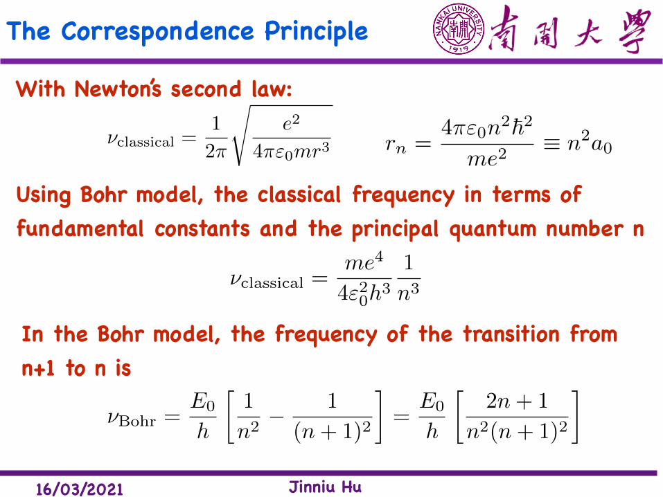
With Newton’s second law:
⌫classical =1
2⇡
se2
4⇡"0mr3
Using Bohr model, the classical frequency in terms of fundamental constants and the principal quantum number n
⌫classical =me4
4"20h3
1
n3
In the Bohr model, the frequency of the transition from n+1 to n is
⌫Bohr =E0
h
1
n2� 1
(n+ 1)2
�=
E0
h
2n+ 1
n2(n+ 1)2
�
rn =4⇡"0n2~2
me2⌘ n2a0
16/03/2021 Jinniu Hu
The Correspondence Principle
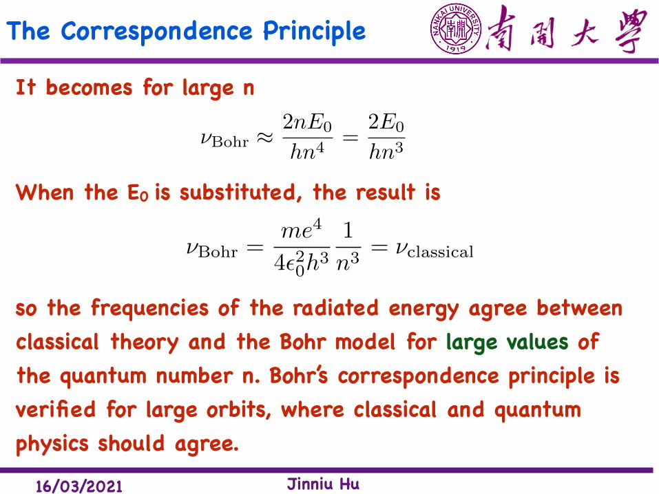
It becomes for large n
⌫Bohr ⇡2nE0
hn4=
2E0
hn3
When the E0 is substituted, the result is
⌫Bohr =me4
4✏20h3
1
n3= ⌫classical
so the frequencies of the radiated energy agree between classical theory and the Bohr model for large values of the quantum number n. Bohr’s correspondence principle is verified for large orbits, where classical and quantum physics should agree.
16/03/2021 Jinniu Hu
The Successes of Bohr Model
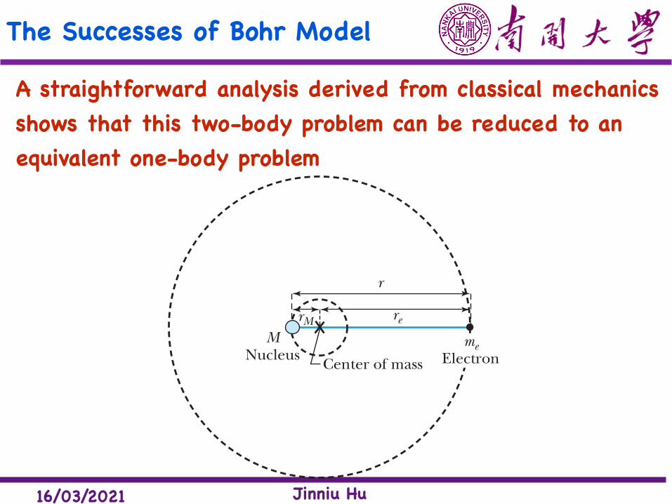
A straightforward analysis derived from classical mechanics shows that this two-body problem can be reduced to an equivalent one-body problem
148 Chapter 4 Structure of the Atom
theory in Chapter 6. Wavelength measurements for the atomic spectrum of hy-drogen are precise and exhibit a small disagreement with the Bohr model results just presented. These disagreements can be corrected by looking more carefully at our original assumptions, one of which was to assume an infinite nuclear mass.
Reduced Mass CorrectionThe electron and hydrogen nucleus actually revolve about their mutual center of mass as shown in Figure 4.17. This is a two-body problem, and our previous analysis should be in terms of re and rM instead of just r. A straightforward analysis derived from classical mechanics shows that this two-body problem can be re-duced to an equivalent one-body problem in which the motion of a particle of mass me moves in a central force field around the center of mass. The only change required in the results of Section 4.4 is to replace the electron mass me by its reduced mass me where
me !me
Mme " M
!me
1 "me
M
(4.36)
and M is the mass of the nucleus (see Problem 53). In the case of the hydro-gen atom, M is the proton mass, and the correction for the hydrogen atom is me ! 0.999456 me. This difference can be measured experimentally. The Rydberg constant for infinite nuclear mass, R q, defined in Equation (4.29), should be replaced by R, where
R !me
me Rq !
1
1 "me
M
Rq !me e 4
4pc U314pP0 22 (4.37)
The Rydberg constant for hydrogen is R H ! 1.096776 # 107 m$1.
Reduced mass
meElectron
rerM
r
MNucleus Center of mass
Figure 4.17 Because the nu-cleus does not actually have an infinite mass, the electron and nucleus rotate about a common center of mass that is located very near the nucleus. This diagram is a very simplistic view of a hydro-gen atom.
03721_ch04_127-161.indd 14803721_ch04_127-161.indd 148 9/29/11 9:36 AM9/29/11 9:36 AM
16/03/2021 Jinniu Hu
The Successes of Bohr Model
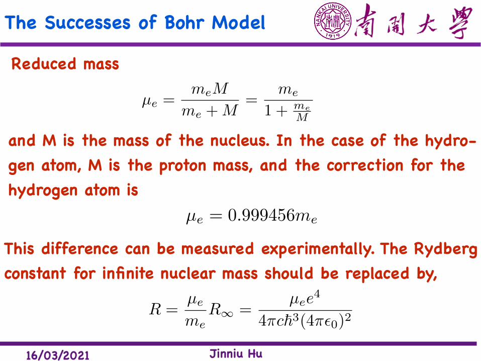
Reduced mass
µe =meM
me +M=
me
1 + meM
and M is the mass of the nucleus. In the case of the hydro- gen atom, M is the proton mass, and the correction for the hydrogen atom is
µe = 0.999456me
This difference can be measured experimentally. The Rydberg constant for infinite nuclear mass should be replaced by,
R =µe
meR1 =
µee4
4⇡c~3(4⇡✏0)2
16/03/2021 Jinniu Hu
The Successes of Bohr Model
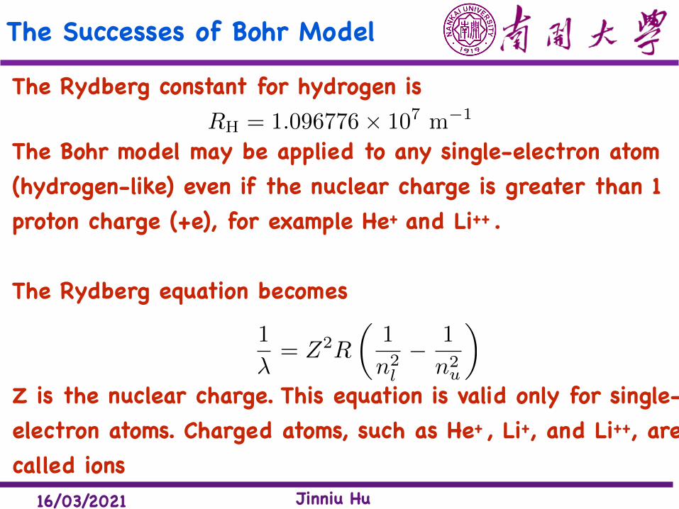
The Rydberg constant for hydrogen isRH = 1.096776⇥ 107 m�1
The Bohr model may be applied to any single-electron atom (hydrogen-like) even if the nuclear charge is greater than 1 proton charge (+e), for example He+ and Li++ .
The Rydberg equation becomes
Z is the nuclear charge. This equation is valid only for single-electron atoms. Charged atoms, such as He+ , Li+, and Li++, are called ions
1
�= Z2R
✓1
n2l
� 1
n2u
◆
16/03/2021 Jinniu Hu
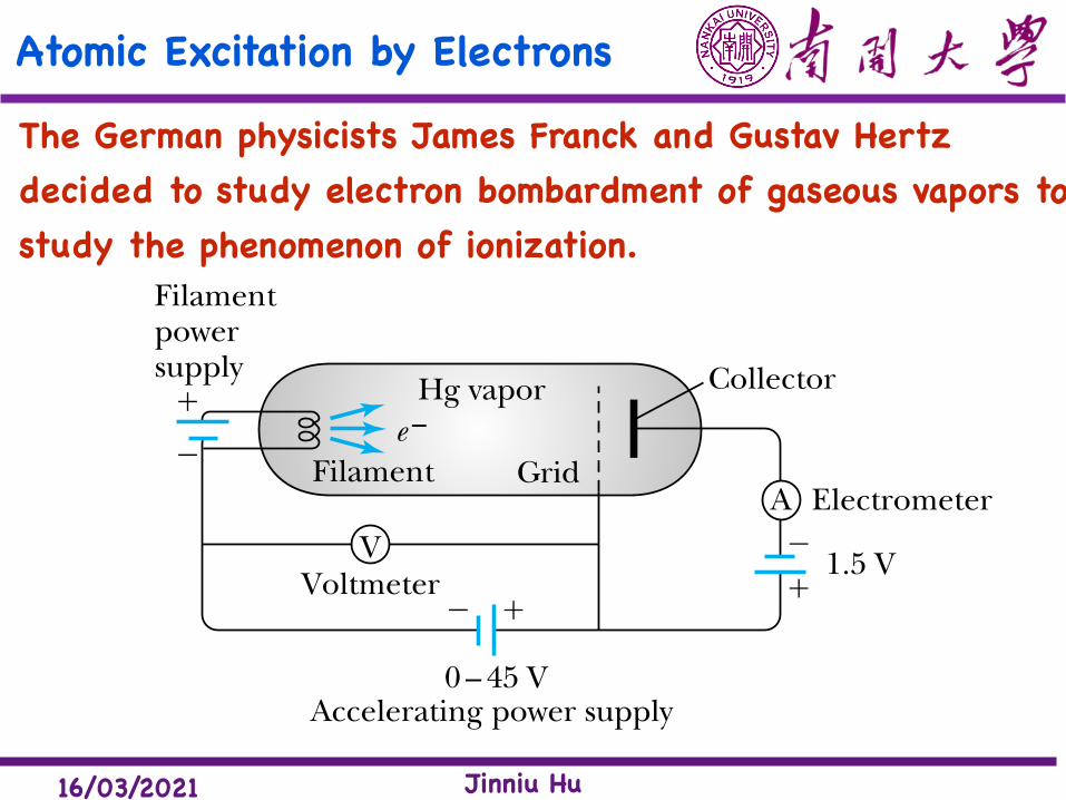
Atomic Excitation by Electrons The German physicists James Franck and Gustav Hertz decided to study electron bombardment of gaseous vapors to study the phenomenon of ionization.
4.7 Atomic Excitation by Electrons 155
electron current registered in the electrometer continued to increase as V in-creased. However, as the accelerating voltage increased above 5 V, there was a sudden drop in the current (see Figure 4.21, which was constructed using data taken by students performing this experiment). As the accelerating voltage con-tinued to increase above 5 V, the current increased again, but suddenly dropped above 10 V. Franck and Hertz first interpreted this behavior as the onset of ion-ization of the Hg atom; that is, an atomic electron is given enough energy to remove it from the Hg, leaving the atom ionized. They later realized that the Hg atom was actually being excited to its first excited state.
We can explain the experimental results of Franck and Hertz within the context of Bohr’s picture of quantized atomic energy levels. In the most popular representation of atomic energy states, we say that the atom, when all the elec-trons are in their lowest possible energy states, is the ground state. We define this energy E0 to be zero. The first quantized energy state above the ground state is called the first excited state, and it has energy E1. The energy difference E1 ! 0 " E1 is called the excitation energy of the state E1. We show the position of one
Collector
Filament!power!supply
Voltmeter
Grid
Hg vapore!
Filament
VA Electrometer
1.5 V
0 – 45 VAccelerating power supply
!
##
#
!
!
Figure 4.20 Schematic diagram of apparatus used in an undergraduate physics laboratory for the Franck-Hertz experiment. The hot filament produces electrons, which are accelerated through the mercury vapor toward the grid. A decelerating voltage between grid and collector prevents the electrons from registering in the electrometer unless the electron has a certain minimum energy.
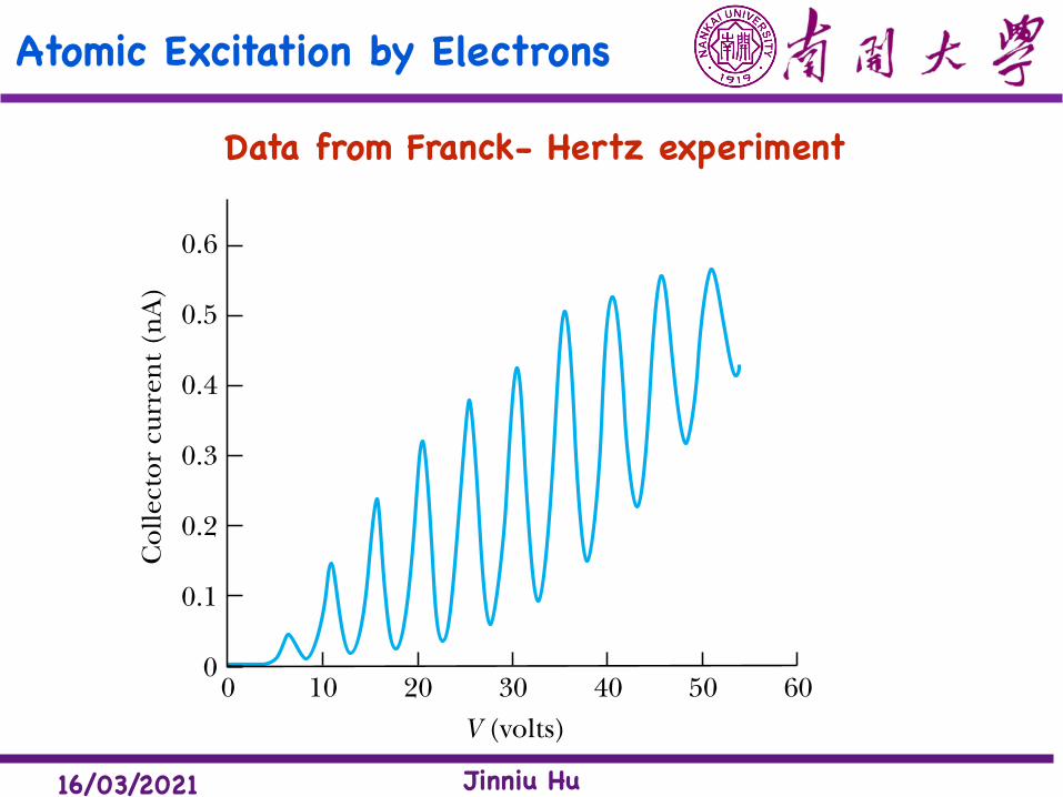
Figure 4.21 Data from an un-dergraduate student’s Franck-Hertz experiment using appara-tus similar to that shown in Figure 4.20. The energy differ-ence between peaks is about 5 V, but the first peak is not at 5 V be-cause of the work function differ-ences of the metals used for the filament and grid.
0
0.1
0.2
0.3
0.4
Col
lect
or c
urre
nt (
nA)
0.5
0.6
V (volts)0 10 20 30 40 50 60
03721_ch04_127-161.indd 15503721_ch04_127-161.indd 155 9/29/11 9:36 AM9/29/11 9:36 AM
16/03/2021 Jinniu Hu
Atomic Excitation by Electrons
4.7 Atomic Excitation by Electrons 155
electron current registered in the electrometer continued to increase as V in-creased. However, as the accelerating voltage increased above 5 V, there was a sudden drop in the current (see Figure 4.21, which was constructed using data taken by students performing this experiment). As the accelerating voltage con-tinued to increase above 5 V, the current increased again, but suddenly dropped above 10 V. Franck and Hertz first interpreted this behavior as the onset of ion-ization of the Hg atom; that is, an atomic electron is given enough energy to remove it from the Hg, leaving the atom ionized. They later realized that the Hg atom was actually being excited to its first excited state.
We can explain the experimental results of Franck and Hertz within the context of Bohr’s picture of quantized atomic energy levels. In the most popular representation of atomic energy states, we say that the atom, when all the elec-trons are in their lowest possible energy states, is the ground state. We define this energy E0 to be zero. The first quantized energy state above the ground state is called the first excited state, and it has energy E1. The energy difference E1 ! 0 " E1 is called the excitation energy of the state E1. We show the position of one
Collector
Filament!power!supply
Voltmeter
Grid
Hg vapore!
Filament
VA Electrometer
1.5 V
0 – 45 VAccelerating power supply
!
##
#
!
!
Figure 4.20 Schematic diagram of apparatus used in an undergraduate physics laboratory for the Franck-Hertz experiment. The hot filament produces electrons, which are accelerated through the mercury vapor toward the grid. A decelerating voltage between grid and collector prevents the electrons from registering in the electrometer unless the electron has a certain minimum energy.
Figure 4.21 Data from an un-dergraduate student’s Franck-Hertz experiment using appara-tus similar to that shown in Figure 4.20. The energy differ-ence between peaks is about 5 V, but the first peak is not at 5 V be-cause of the work function differ-ences of the metals used for the filament and grid.
0
0.1
0.2
0.3
0.4
Col
lect
or c
urre
nt (
nA)
0.5
0.6
V (volts)0 10 20 30 40 50 60
03721_ch04_127-161.indd 15503721_ch04_127-161.indd 155 9/29/11 9:36 AM9/29/11 9:36 AM
Data from Franck- Hertz experiment
16/03/2021 Jinniu Hu
Atomic Excitation by Electrons
We can explain the experimental results of Franck and Hertz within the context of Bohr’s picture of quantized atomic energy levels.
In the most popular representation of atomic energy states, we say that the atom, when all the electrons are in their lowest possible energy states, is the ground state. The first quantized energy state above the ground state is called the first excited state.
16/03/2021 Jinniu Hu
Atomic Excitation by Electrons 156 Chapter 4 Structure of the Atom
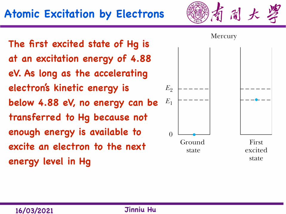
electron in an energy-level diagram of Hg in Figure 4.22 in both the ground state and first excited state. The first excited state of Hg is at an excitation energy of 4.88 eV. As long as the accelerating electron’s kinetic energy is below 4.88 eV, no energy can be transferred to Hg because not enough energy is available to excite an electron to the next energy level in Hg. The Hg atom is so much more massive than the electron that almost no kinetic energy is transferred to the re-coil of the Hg atom; the collision is elastic. The electron can only bounce off the Hg atom and continue along a new path with about the same kinetic energy. If the electron gains at least 4.88 eV of kinetic energy from the accelerating poten-tial, it can transfer 4.88 eV to an electron in Hg, promoting it to the first excited state. This is an inelastic collision. A bombarding electron that has lost energy in an inelastic collision then has too little energy (after it passes the grid) to reach the collector. Above 4.88 V, the current dramatically drops because the inelasti-cally scattered electrons no longer reach the collector.
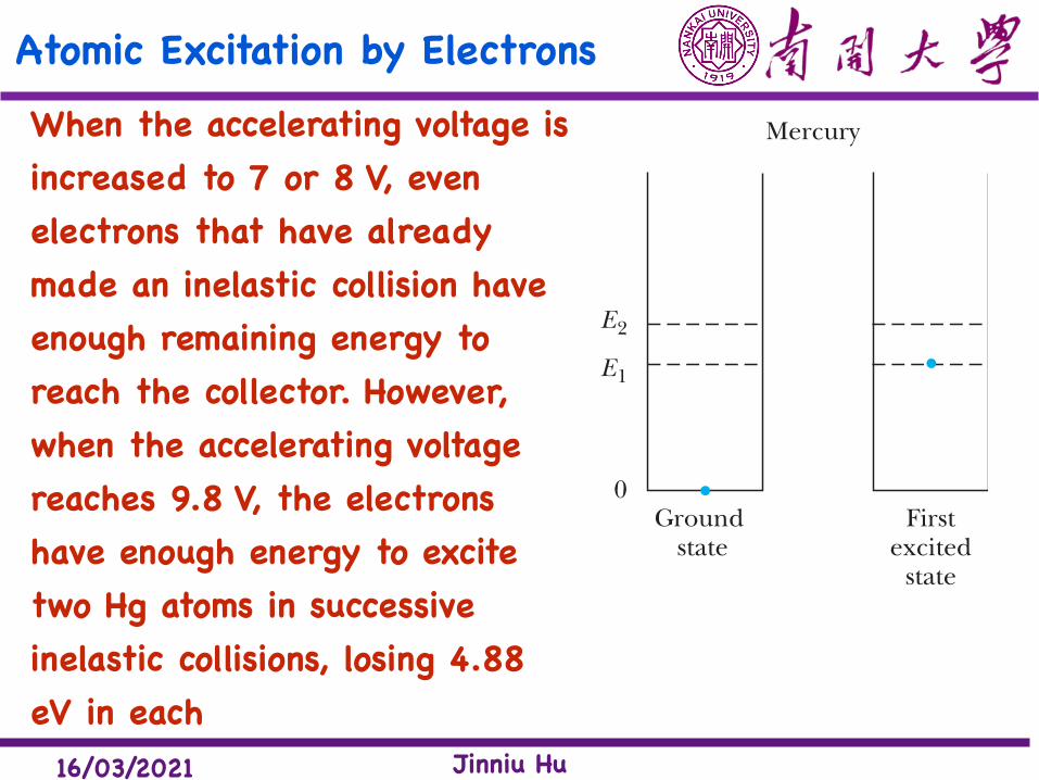
When the accelerating voltage is increased to 7 or 8 V, even electrons that have already made an inelastic collision have enough remaining energy to reach the collector. Once again the current increases with V. However, when the ac-celerating voltage reaches 9.8 V, the electrons have enough energy to excite two Hg atoms in successive inelastic collisions, losing 4.88 eV in each (2 ! 4.88 eV " 9.76 eV). The current drops sharply again. As we see in Figure 4.21, even with student apparatus it is possible to observe several successive excitations as the accelerating voltage is increased. Notice that the energy differences between peaks are typically 4.9 eV. The first peak does not occur at 4.9 eV because of the difference in the work functions between the dissimilar metals used as cathode and anode. Other highly excited states in Hg can also be excited in an inelastic collision, but the probability of exciting them is much smaller than that for the first excited state. Franck and Hertz, however, were able to detect them.
The Franck-Hertz experiment convincingly proved the quantization of atomic electron energy levels. The bombarding electron’s kinetic energy can change only by certain discrete amounts determined by the atomic energy levels of the mercury atom. They performed the experiment with gases of several other elements and obtained similar results.
Would it be experimentally possible to observe radiation emitted from the first excited state of Hg after it was pro-duced by an electron collision?
Solution If the collision of the bombarding electron with the mercury atom is elastic, mercury will be left in its ground state. If the collision is inelastic, however, the mercury atom will end up in its excited state at 4.9 eV (see Figure 4.22). The mercury atom will not exist long in its first excited state
and should decay quickly (!10#8 s) back to the ground state. Franck and Hertz considered this possibility and looked for x rays. They observed no radiation emitted when the electron’s kinetic energy was below about 5 V, but as soon as the current dropped as the voltage went past 5 V, indicating excitation of Hg, an emission line of wavelength 254 nm (ultraviolet) was observed. Franck and Hertz set E " 4.88 eV " hf " (hc)/l and showed that the value of h determined from l " 254 nm was in good agreement with values of Planck’s constant determined by other means.
CONCEPTUAL EXAMPLE 4 .11
Ground !state
E2
E1
0First!
excited!state
Mercury
Figure 4.22 A valence electron is shown in the ground state of mercury on the left. On the right side the electron has been ele-vated to the first excited state af-ter a bombarding electron scat-tered inelastically from the mercury atom.
03721_ch04_127-161.indd 15603721_ch04_127-161.indd 156 9/29/11 9:36 AM9/29/11 9:36 AM
The first excited state of Hg is at an excitation energy of 4.88 eV. As long as the accelerating electron’s kinetic energy is below 4.88 eV, no energy can be transferred to Hg because not enough energy is available to excite an electron to the next energy level in Hg
16/03/2021 Jinniu Hu
Atomic Excitation by Electrons 156 Chapter 4 Structure of the Atom
electron in an energy-level diagram of Hg in Figure 4.22 in both the ground state and first excited state. The first excited state of Hg is at an excitation energy of 4.88 eV. As long as the accelerating electron’s kinetic energy is below 4.88 eV, no energy can be transferred to Hg because not enough energy is available to excite an electron to the next energy level in Hg. The Hg atom is so much more massive than the electron that almost no kinetic energy is transferred to the re-coil of the Hg atom; the collision is elastic. The electron can only bounce off the Hg atom and continue along a new path with about the same kinetic energy. If the electron gains at least 4.88 eV of kinetic energy from the accelerating poten-tial, it can transfer 4.88 eV to an electron in Hg, promoting it to the first excited state. This is an inelastic collision. A bombarding electron that has lost energy in an inelastic collision then has too little energy (after it passes the grid) to reach the collector. Above 4.88 V, the current dramatically drops because the inelasti-cally scattered electrons no longer reach the collector.
When the accelerating voltage is increased to 7 or 8 V, even electrons that have already made an inelastic collision have enough remaining energy to reach the collector. Once again the current increases with V. However, when the ac-celerating voltage reaches 9.8 V, the electrons have enough energy to excite two Hg atoms in successive inelastic collisions, losing 4.88 eV in each (2 ! 4.88 eV " 9.76 eV). The current drops sharply again. As we see in Figure 4.21, even with student apparatus it is possible to observe several successive excitations as the accelerating voltage is increased. Notice that the energy differences between peaks are typically 4.9 eV. The first peak does not occur at 4.9 eV because of the difference in the work functions between the dissimilar metals used as cathode and anode. Other highly excited states in Hg can also be excited in an inelastic collision, but the probability of exciting them is much smaller than that for the first excited state. Franck and Hertz, however, were able to detect them.
The Franck-Hertz experiment convincingly proved the quantization of atomic electron energy levels. The bombarding electron’s kinetic energy can change only by certain discrete amounts determined by the atomic energy levels of the mercury atom. They performed the experiment with gases of several other elements and obtained similar results.
Would it be experimentally possible to observe radiation emitted from the first excited state of Hg after it was pro-duced by an electron collision?
Solution If the collision of the bombarding electron with the mercury atom is elastic, mercury will be left in its ground state. If the collision is inelastic, however, the mercury atom will end up in its excited state at 4.9 eV (see Figure 4.22). The mercury atom will not exist long in its first excited state
and should decay quickly (!10#8 s) back to the ground state. Franck and Hertz considered this possibility and looked for x rays. They observed no radiation emitted when the electron’s kinetic energy was below about 5 V, but as soon as the current dropped as the voltage went past 5 V, indicating excitation of Hg, an emission line of wavelength 254 nm (ultraviolet) was observed. Franck and Hertz set E " 4.88 eV " hf " (hc)/l and showed that the value of h determined from l " 254 nm was in good agreement with values of Planck’s constant determined by other means.
CONCEPTUAL EXAMPLE 4 .11
Ground !state
E2
E1
0First!
excited!state
Mercury
Figure 4.22 A valence electron is shown in the ground state of mercury on the left. On the right side the electron has been ele-vated to the first excited state af-ter a bombarding electron scat-tered inelastically from the mercury atom.
03721_ch04_127-161.indd 15603721_ch04_127-161.indd 156 9/29/11 9:36 AM9/29/11 9:36 AM
When the accelerating voltage is increased to 7 or 8 V, even electrons that have already made an inelastic collision have enough remaining energy to reach the collector. However, when the accelerating voltage reaches 9.8 V, the electrons have enough energy to excite two Hg atoms in successive inelastic collisions, losing 4.88 eV in each
16/03/2021 Jinniu Hu
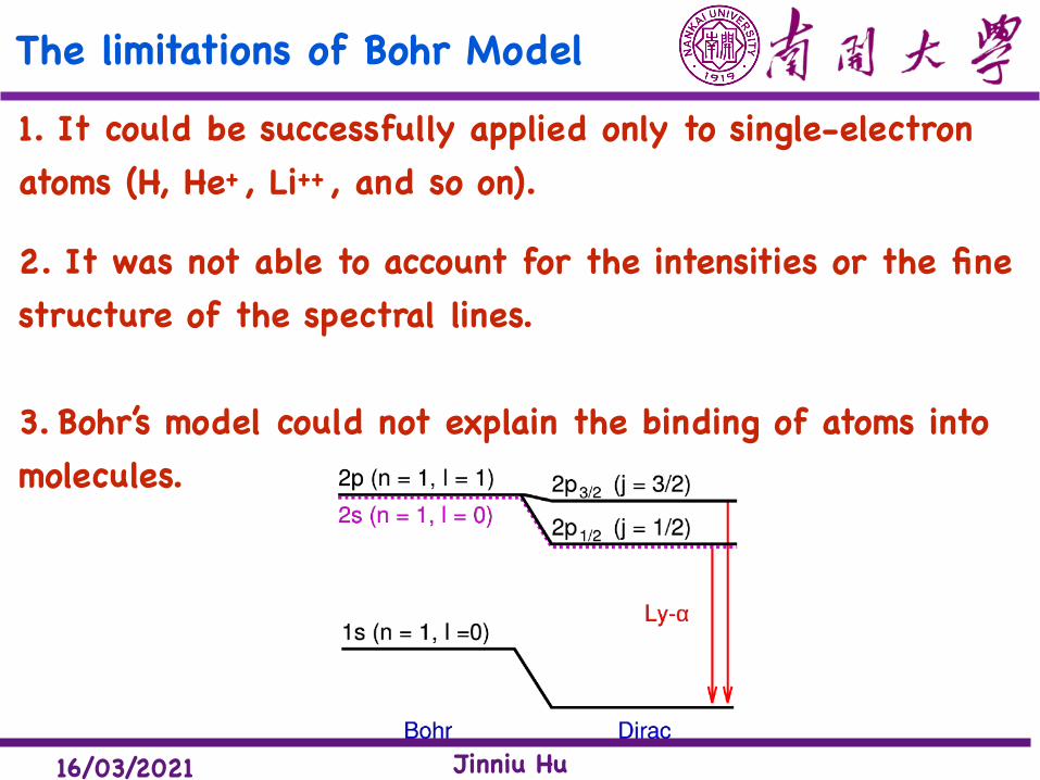
The limitations of Bohr Model 1. It could be successfully applied only to single-electron atoms (H, He+ , Li++ , and so on).
2. It was not able to account for the intensities or the fine structure of the spectral lines.
3. Bohr’s model could not explain the binding of atoms into molecules.
16/03/2021 Jinniu Hu
The extension of Bohr model Sommerfeld succeeded partially in explaining the observed fine structure of spectral lines by introducing the following main modifications in Bohr’s theory:
1.Sommerfeld suggested that the path of an electron around the nucleus, in general, is an ellipse with the nucleus at one of the foci.
2. Sommerfeld took into account the relativistic variation of the mass of the electron with velocity. Hence this model of the atom is called the relativistic atom model.
16/03/2021 Jinniu Hu
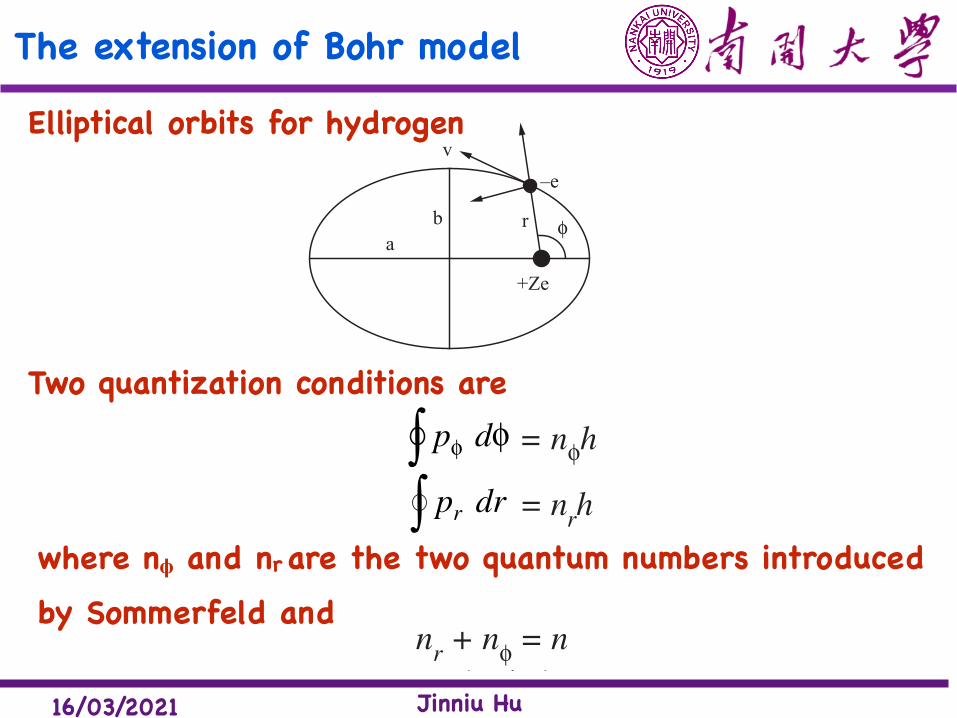
The extension of Bohr model Elliptical orbits for hydrogen
8-f\\N-Solid\SSP2-1.pm7.0 13
!"#$"%&'(&)*'+$,&-*!.,*.!" /0
(vi) The theory cannot be used for the quantitative study of chemical bonding.
(vii) It was found that when electric or magnetic field is applied to the atom, each spectral line issplitted into several lines. The former one is called Stark effect while the later as Zeemaneffect. Bohr’s theory fails to explain these effects.
1$2&-'++"!("345-&!"3)*$#$-*$,&)*'+&+'4"3
According to Bohr, the lines of hydrogen-like spectrum should each have a well-defined wavelength.Careful spectroscopic examination showed that the HD, HE and HJ lines in the hydrogen spectrum arenot single. Each spectral line actually consisted of several very close lines packed together. Michelsonfound that under high resolution, HD line can be resolved into two close components, with a wavelengthseparation of 0.013 nm. This is called the fine structure of the spectral lines. Bohr’s theory could notexplain this fine structure.
Sommerfeld succeeded partially in explaining the observed fine structure of spectral lines byintroducing the following main modifications in Bohr’s theory:
(i) Sommerfeld suggested that the path of an electron around the nucleus, in general, is an ellipsewith the nucleus at one of the foci. The circular orbits of Bohr are a special case of this.
(ii) The velocity of the electron moving in an elliptical orbit varies considerably at different partsof the orbit. This causes relativistic variation in the mass of the moving electron. ThereforeSommerfeld took into account the relativistic variation of the mass of the electron with velocity.Hence this model of the atom is called the relativistic atom model.
1$$2&"33$6*$,)3&'!7$*-&('!&894!':";
An electron moving in the field of the nucleus describes elliptical orbits, with the nucleus at one focus.Circular orbits are only special cases of ellipses. When the electron moves along a circular orbit, the angularcoordinate is sufficient to describe its motion. In an elliptical orbit, the position of the electron at any timeinstant is fixed by two coordinates namely the angular coordinate (I) and the radial coordinate (r). Here r isthe radius vector and I is the angle which the radius vector makes with the major axis of the ellipse.
Consider an electron of mass m and linear tangential velocityv revolving in the elliptical orbit. This tangential velocity of theelectron can be resolved into two components: One along the radiusvector called radial velocity and the other perpendicular to the radiusvector called the transverse velocity. Corresponding to thesevelocities, the electron has two momenta: One along the radiusvector called radial momentum and the other perpendicular to theradius vector known as azimuthal momentum or angular momentum.So in the case of elliptic motion, both the angle�I and the radiusvector r vary periodically, as shown in Fig. 2.5.
Thus, the momenta associated with both these coordinates (I�and r) may be quantised inaccordance with Bohr’s quantum condition. The two quantisation conditions are
p dI I! = nIh (2.17)
p drr! = nrh (2.18)
(<=2&>2?&!"##$%&$'()*+#"($'
"&++,-$+.,"#
ab
v
r φ
+Ze
–e
Two quantization conditions are
8-f\\N-Solid\SSP2-1.pm7.0 13
!"#$"%&'(&)*'+$,&-*!.,*.!" /0
(vi) The theory cannot be used for the quantitative study of chemical bonding.
(vii) It was found that when electric or magnetic field is applied to the atom, each spectral line issplitted into several lines. The former one is called Stark effect while the later as Zeemaneffect. Bohr’s theory fails to explain these effects.
1$2&-'++"!("345-&!"3)*$#$-*$,&)*'+&+'4"3
According to Bohr, the lines of hydrogen-like spectrum should each have a well-defined wavelength.Careful spectroscopic examination showed that the HD, HE and HJ lines in the hydrogen spectrum arenot single. Each spectral line actually consisted of several very close lines packed together. Michelsonfound that under high resolution, HD line can be resolved into two close components, with a wavelengthseparation of 0.013 nm. This is called the fine structure of the spectral lines. Bohr’s theory could notexplain this fine structure.
Sommerfeld succeeded partially in explaining the observed fine structure of spectral lines byintroducing the following main modifications in Bohr’s theory:
(i) Sommerfeld suggested that the path of an electron around the nucleus, in general, is an ellipsewith the nucleus at one of the foci. The circular orbits of Bohr are a special case of this.
(ii) The velocity of the electron moving in an elliptical orbit varies considerably at different partsof the orbit. This causes relativistic variation in the mass of the moving electron. ThereforeSommerfeld took into account the relativistic variation of the mass of the electron with velocity.Hence this model of the atom is called the relativistic atom model.
1$$2&"33$6*$,)3&'!7$*-&('!&894!':";
An electron moving in the field of the nucleus describes elliptical orbits, with the nucleus at one focus.Circular orbits are only special cases of ellipses. When the electron moves along a circular orbit, the angularcoordinate is sufficient to describe its motion. In an elliptical orbit, the position of the electron at any timeinstant is fixed by two coordinates namely the angular coordinate (I) and the radial coordinate (r). Here r isthe radius vector and I is the angle which the radius vector makes with the major axis of the ellipse.
Consider an electron of mass m and linear tangential velocityv revolving in the elliptical orbit. This tangential velocity of theelectron can be resolved into two components: One along the radiusvector called radial velocity and the other perpendicular to the radiusvector called the transverse velocity. Corresponding to thesevelocities, the electron has two momenta: One along the radiusvector called radial momentum and the other perpendicular to theradius vector known as azimuthal momentum or angular momentum.So in the case of elliptic motion, both the angle�I and the radiusvector r vary periodically, as shown in Fig. 2.5.
Thus, the momenta associated with both these coordinates (I�and r) may be quantised inaccordance with Bohr’s quantum condition. The two quantisation conditions are
p dI I! = nIh (2.17)
p drr! = nrh (2.18)
(<=2&>2?&!"##$%&$'()*+#"($'
"&++,-$+.,"#
ab
v
r φ
+Ze
–e
where n" and nr are the two quantum numbers introduced by Sommerfeld and
8-f\\N-Solid\SSP2-1.pm7.0 14
!" #$%&'(#)*)+(,-.#&/#
where nI and nr are the two quantum numbers introduced by Sommerfeld. Since they stand for oneperiodic system, nr + nI = n. Here nr is known as radial quantum number, nI as angular or azimuthalquantum number and n is known as principal quantum number.
Now, we have to quantise the momenta associated with both the radial and angular coordinates.The two equations are
p dI I! = nIh
and p drr! = nrh
The integrals are taken over one complete cycle of variation of the respective coordinates. BothnI and nr are integers. Furthermore, the sum of nr and nI is equal to the principal quantum number n.
The force on the electron is due to the electrostatic attraction to the nucleus and acts along theradius vector. There is no force at right angles to this radius vector, so the transverse component of theacceleration is zero throughout the atom. Hence
12
2
r
ddt
rddtI"
#$%&' is zero.
Therefore r2 ddtI(
)*+ and so mr2
ddtI"
#$%&' must be a constant.
Equation (2.17) can be easily evaluated. Thus,
p dI
SI
0
2! = nIh
pI = nI�h
2S()*+ (2.19)
This equation shows that the angular momentum of the electron is an integral multiple of h
2S.
It is considerably difficult to evaluate the integral in equation (2.18). However, an attempt ismade here. The polar equation to the ellipse is
1r
=1
1 2
� H IH
cos( – )a
(2.20)
where a is the semimajor axis and H is the eccentricity. Thus differentiating this equation with respect toI, we get
12r
()*+
dr
dI(),*+- =
H IH
sin( – )a 1 2
1r
dr
dI(),*+-
=r
aH I
Hsin
( – )1 2 (2.21)
16/03/2021 Jinniu Hu
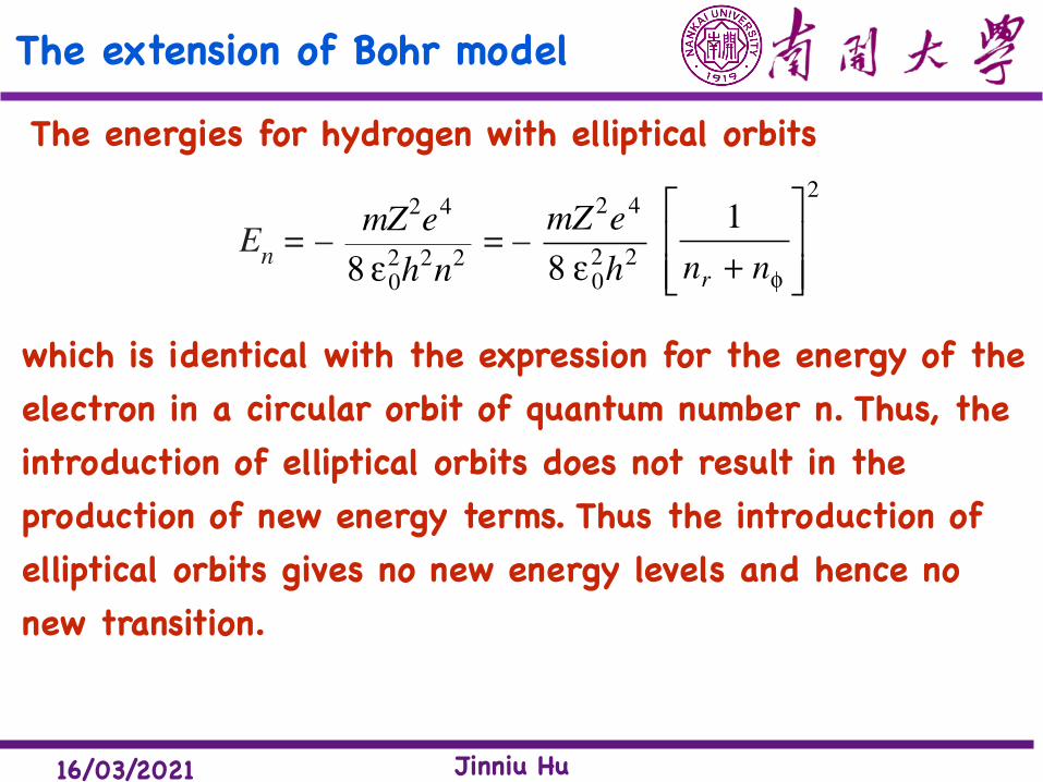
The extension of Bohr model The energies for hydrogen with elliptical orbits
8-f\\N-Solid\SSP2-2.pm7.0 20
!" #$%&'(#)*)+(,-.#&/#
=r
a
2 2
2 2 21HH( – )
– r
a
2
2 2 21( – )H +
21 2
ra( – )H
– 1
=r r
a
2 2 2
2 2 21H
H–
( – ) +
21 2
ra( – )H
– 1
= – r
a
2 2
2 2 2
11( – )( – )
HH
+ 2
1 2
ra( – )H
– 1 (2.34)
Equating the coefficients of r2 and r in equations (2.34) and (2.32), we get
22
mE
pn
I= –
112 2a ( – )H
(2.35)
andmZe
p
2
022S H I
=2
1 2a( – )H(2.36)
Thus equation (2.35) becomes
En = – p
maI
H
2
2 22 1( – )(2.37)
Substituting the value of ( – )1 2H from equation (2.36) in equation (2.37), we get
En = – p
maI2
22
amZe
p
2
024S H I
!
"##
$
%&&
En = – Zea
2
08 S H(2.38)
Again substituting for a from equation (2.36), we get
En = – Ze2
08 S H'()
*+,
mZe
p
2
022 S H I
'()
*+,
12
2– H'()
*+,
En = – mZ e2 4
20232 S H
!"#
$%&
( – )1 2
2
H
Ip
Substituting for ( – )1 2H and pI2 from equations (2.25) and (2.19) respectively, we get
En = – mZ e2 4
20232 S H
!"#
$%&
n
nI'
()*+,
2 22
S
In h
'()
*+,
En = – mZ e
h n
2 4
02 2 28 H
= – mZ e
h
2 4
02 28 H
1
2
n nr �
!
"##
$
%&&I
(2.39)
which is identical with the expression for the energy of the electron in a circular orbit of quantumnumber n. Thus, the introduction of elliptical orbits does not result in the production of new energyterms; hence no new spectral lines are to be expected because of this multiplicity of orbits. Thus theintroduction of elliptical orbits gives no new energy levels and hence no new transition. HenceSommerfeld’s attempt to explain the fine structure of spectral lines failed. But soon, on the basis of
which is identical with the expression for the energy of the electron in a circular orbit of quantum number n. Thus, the introduction of elliptical orbits does not result in the production of new energy terms. Thus the introduction of elliptical orbits gives no new energy levels and hence no new transition.
16/03/2021 Jinniu Hu
The extension of Bohr model
8-f\\N-Solid\SSP2-2.pm7.0 22
!! "#$%&'"()(*'+,-"%."
corresponding to these letters are 1, 2, 3, 4, etc. respectively. In this notation, the orbit determined by n = 3and nI = 1 is represented by 3s. Similarly 4d will represent the orbit n = 4 and nI = 3. These orbits arerepresented in Fig. 2.6.
The transitions between the orbits n = 3 and n = 2 giving HD line can now take place in sixdifferent ways. However, all these transitions have the same energy E3 – E2 and hence give rise to asingle frequency for the HD line, according to the frequency condition. No new lines, which wouldexplain the fine structure are therefore predicted.
33
32
31
b
a3d 3p 3s
n = 3
n = 1φ
b = a3n = 3
n = 2φ
b = 2a3
n = 3n = 3φ
b = a
a = 9rBa = 4rBa = rB
1122
21
2p 2s1s a ab
n = 1n = 1φ
b = a
n = 2n = 2φ
b = a
n = 2n = 1φb = a
2
/012'!23'!""#$%#&'"()*+,-.*//0,10"2(*,3#%4(1*,(+52,*607
4%52 "#66*7/*$&8"' 7*$)(%5%"(%.' .#77*.(%#9
The velocity of an electron moving in an elliptical orbit varies from point to point in the orbit, being amaximum when the electron is nearest to the nucleus and a minimum when it is farther away from the
nucleus. Furthermore, this velocity is quite large c
137!"
#$ . According to the theory of relativity, the variation
of velocity means variation of mass of the electron.
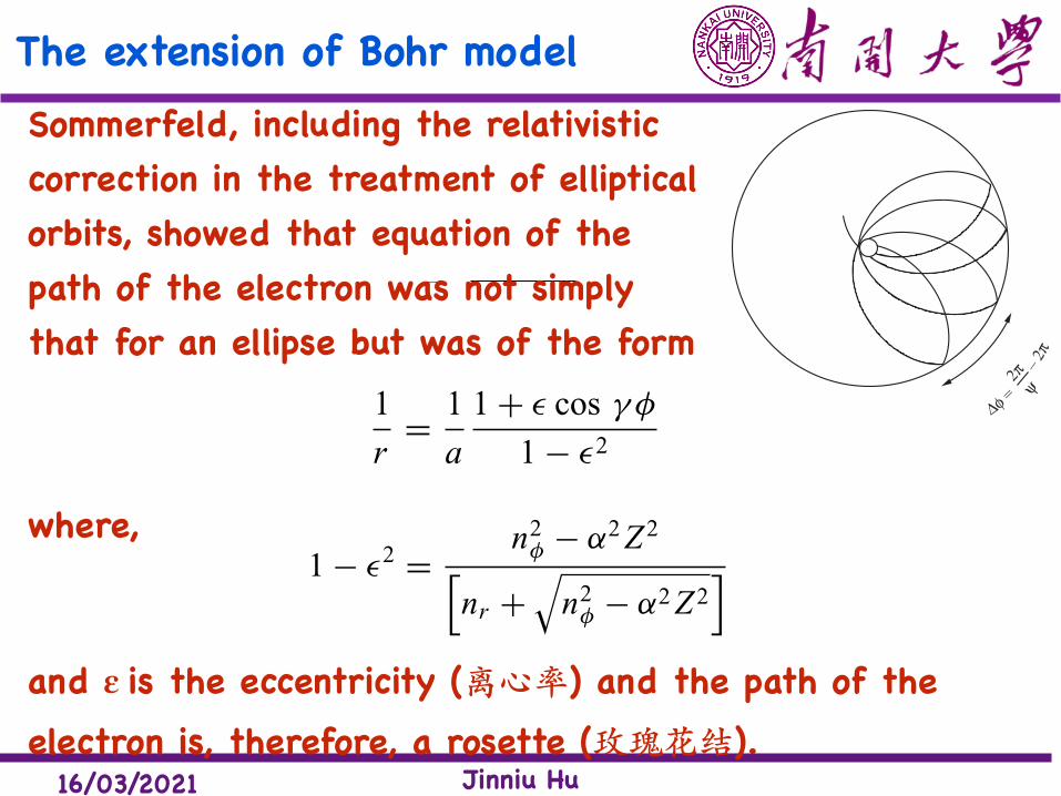
Sommerfeld, including the relativistic correction in thetreatment of elliptical orbits, showed that equation of the pathof the electron was not simply that for an ellipse but was of theform
1r
=1
1 2
� H \IH
cos( – )a
where \ is given by
\ 2 = 1 – Ze
pc
2
0
2
4S H%&'
()*
This is the equation of an ellipse which precesses, i.e.,the major axis turns slowly about the focus (the nucleus) in the
/012'!2:'8*40%%0($'%+(*1(%+0(0"0&%,*7
'3*9%(%+0(79&"094
∆φ =
2πψ
–2π
Sommerfeld, including the relativistic correction in the treatment of elliptical orbits, showed that equation of the path of the electron was not simply that for an ellipse but was of the form
where,
and # is the eccentricity (���) and the path of the electron is, therefore, a rosette (����).
97 5.3 Sommerfeld and the !ne-structure constant
Fig. 5.3 Illustrating the precession of the elliptical orbits when the e"ects of special relativity are taken into account. Thisdiagram appears as Fig. 110 in Sommerfeld’s book Atombau und Spektrallinien (Sommerfeld, 1919).
where p is now the relativistic three-momentum and is quantised according to the rule∮p dφ = nφh. p0 is defined to be the quantity p0 = Ze2/4πε0c. In the case of circular
Bohr orbits, it is straightforward to show that γ = (1 − v2/c2)1/2, in other words, the inverseof my normal convention for the Lorentz factor γ = (1 − v2/c2)−1/2. Just for this section,we will use γ in Sommerfeld’s sense. Inspection of (5.29) shows that, since γ ≤ 1, the orbitdoes not close up after φ = 2π radians, but after γφ = 2π radians. This slight change perorbit is illustrated by the angle %φ in Fig. 5.3. The orbits return to the standard ellipticalform however if we introduce the coordinate ψ = γφ. Sommerfeld shows that the equationfor the ellipse now becomes
1r
= 1a
1 + ε cos γφ
1 − ε2, (5.31)
while the momenta corresponding to r,φ are
pφ = mr2φ , pr = mr , (5.32)
where the momenta are relativistic three-momenta, that is, in (5.32) m = me(1 − v2/c2)−1/2.The one important difference is that the quantisation condition in the radial direction nowcorresponds to the integration over a single ellipse in the ψ coordinate, that is,
∫ 2π
φ=0pφ dφ = nφh and
∫ ψ=2π
ψ=0pr dr = nr h . (5.33)
Carrying out the same procedure as in the non-relativistic case, Sommerfeld found that theellipticities of the orbits are given by
1 − ε2 =n2
φ − α2 Z2
[nr +
√n2
φ − α2 Z2] , (5.34)
where α = e2/2ε0hc is the fine-structure constant, for reasons which will be apparent ina moment. It is already clear that the degeneracy of the energy levels has been relieved
16/03/2021 Jinniu Hu
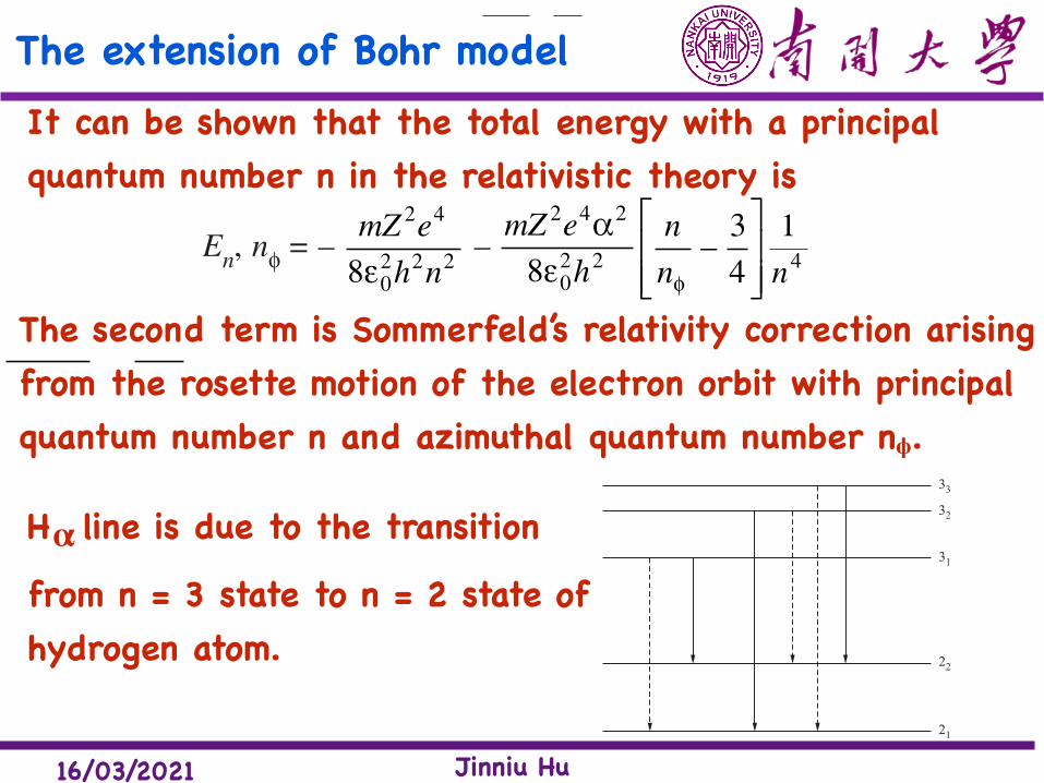
The extension of Bohr model It can be shown that the total energy with a principal quantum number n in the relativistic theory is
8-f\\N-Solid\SSP2-1.pm7.0 23
!"#$"%&'(&)*'+$,&-*!.,*.!" /0
plane of the ellipse. The path of the electron is, therefore, a rosette.It can be shown that the total energy with a principal quantum number n in the relativistic theory is
En, nI = – mZ e
h n
2 4
02 2 28H
– mZ e
h
2 4 2
02 28D
HnnI
–34
!
"##
$
%&&
14n
(2.42)
where D�= e
ch
2
02H =
1137
. D is a dimensionless quantity and is called the fine structure constant.
The first term on the right hand side is the energy of the electron in the orbit with the principalquantum number n according to Bohr’s theory and the second term is Sommerfeld’s relativity correctionarising from the rosette motion of the electron orbit with principal quantum number n and azimuthalquantum number nI.The dependence of the total energy of the electron in its orbit as given by theequation (2.42) results in a splitting of energy levels in the atom. For a given value of n, there will be ncomponents corresponding to the n permitted values of nI. Hence multiplicity of spectral lines shouldappear in hydrogen atom.
1#2&($3"&-*!.,*.!"&'(&4D&5$3"
HD line is due to the transition from n = 3 state to n = 2 state of hydrogen atom. For n = 3, there are threepossible energy levels corresponding to the three values of nI = 1, 2 and 3. Similarly, there are twopossible levels for n = 2. Therefore, theoretically six transitions are possible:
33 o 22 ; 33 o��������o���������o���������o���������o���and these transitions are shown in Fig. 2.8. Actually, the HD line has only three components. To makeexperiment and theory agree, some of the transitions have to be ruled out by some selection rule. The
selection rule is that nI can change only +1 or –1 i.e.,'nI = r 1.
33
32
31
22
21
(672&/28&!"#$%&'&($%)#$*)+(",&**-$).&$-%
1#$2&9!)%:),;-&'(&:'4!<-'++"!("59&)*'+&+'9"5
(i) Bohr’s theory failed to explain the fine structure of spectral lines even in the simplest hydrogenatom.
The second term is Sommerfeld’s relativity correction arising from the rosette motion of the electron orbit with principal quantum number n and azimuthal quantum number n".
8-f\\N-Solid\SSP2-1.pm7.0 23
!"#$"%&'(&)*'+$,&-*!.,*.!" /0
plane of the ellipse. The path of the electron is, therefore, a rosette.It can be shown that the total energy with a principal quantum number n in the relativistic theory is
En, nI = – mZ e
h n
2 4
02 2 28H
– mZ e
h
2 4 2
02 28D
HnnI
–34
!
"##
$
%&&
14n
(2.42)
where D�= e
ch
2
02H =
1137
. D is a dimensionless quantity and is called the fine structure constant.
The first term on the right hand side is the energy of the electron in the orbit with the principalquantum number n according to Bohr’s theory and the second term is Sommerfeld’s relativity correctionarising from the rosette motion of the electron orbit with principal quantum number n and azimuthalquantum number nI.The dependence of the total energy of the electron in its orbit as given by theequation (2.42) results in a splitting of energy levels in the atom. For a given value of n, there will be ncomponents corresponding to the n permitted values of nI. Hence multiplicity of spectral lines shouldappear in hydrogen atom.
1#2&($3"&-*!.,*.!"&'(&4D&5$3"
HD line is due to the transition from n = 3 state to n = 2 state of hydrogen atom. For n = 3, there are threepossible energy levels corresponding to the three values of nI = 1, 2 and 3. Similarly, there are twopossible levels for n = 2. Therefore, theoretically six transitions are possible:
33 o 22 ; 33 o��������o���������o���������o���������o���and these transitions are shown in Fig. 2.8. Actually, the HD line has only three components. To makeexperiment and theory agree, some of the transitions have to be ruled out by some selection rule. The
selection rule is that nI can change only +1 or –1 i.e.,'nI = r 1.
33
32
31
22
21
(672&/28&!"#$%&'&($%)#$*)+(",&**-$).&$-%
1#$2&9!)%:),;-&'(&:'4!<-'++"!("59&)*'+&+'9"5
(i) Bohr’s theory failed to explain the fine structure of spectral lines even in the simplest hydrogenatom.
H !
line is due to the transition
from n = 3 state to n = 2 state of hydrogen atom.
16/03/2021 Jinniu Hu
Alkali Atom
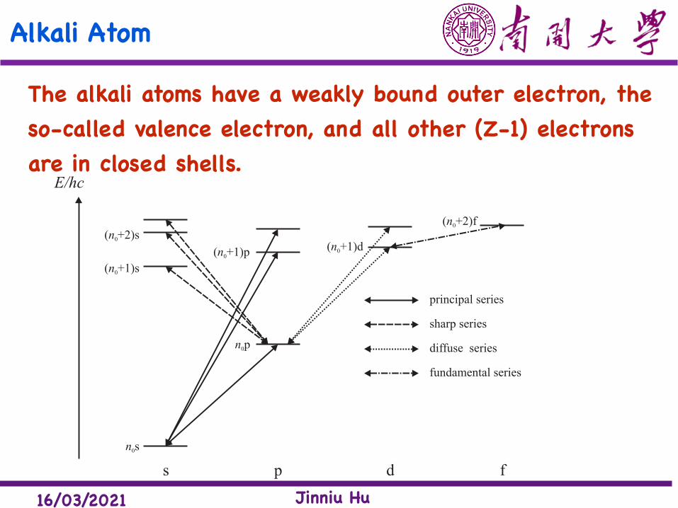
The alkali atoms have a weakly bound outer electron, the so-called valence electron, and all other (Z-1) electrons are in closed shells.
2.2. ATOMIC SPECTRA 55
High-resolution spectroscopy of hydrogen-like atoms such as H, He+, Li2+, Be3+ . . . and
their isotopes continues to stimulate methodological and instrumental progress in electronic
spectroscopy. Measurements on ”artificial” hydrogen-like atoms such as positronium (atom
consisting of an electron and a positron), protonium (atom consisting of a proton and an an-
tiproton), antihydrogen (atom consisting of an antiproton and a positron), muonium (atom
consisting of a positive muon µ+ and an electron), antimuonium (atom consisting of a negative
muon µ− and a positron), etc., have the potential of providing new insights into fundamental
physical laws and symmetries and their violations.
2.2.3 Spectra of alkali-metal atoms
A schematic energy level diagram showing the single-photon transitions that can be observed
in the spectra of the alkali-metal atoms is presented in Figure 2.6. The ground-state config-
uration corresponds to a closed-shell rare-gas-atom configuration with a single valence n0s
electron with n0 = 2, 3, 4, 5 and 6 for Li, Na, K, Rb and Cs, respectively. The energetic
positions of these levels can be determined accurately from Equation (2.2). The Laporte
selection rule (Equation (2.72)) restricts the observable single-photon transitions to those
drawn as double-headed arrows in Figure 2.6. Neglecting the fine and hyperfine structures,
their wave numbers can be determined using:
ν =RM
(n′′ − δ!′′)2− RM
(n′ − δ!′)2. (2.74)
s
E/hc
n0s
( +1)sn0
( +2)sn0
p d f
n0p
( +1)pn0
( +1)dn0
( +2)fn0
principal series
sharp series
diffuse series
fundamental series
Figure 2.6: Schematic diagram showing the transitions that can be observed in the single-
photon spectrum of the alkali-metal atoms.
PCV - Spectroscopy of atoms and molecules
16/03/2021 Jinniu Hu
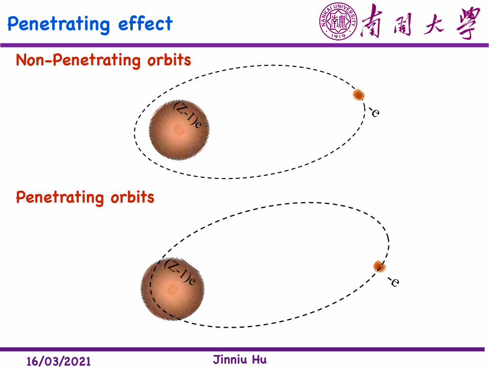
Penetrating effectNon-Penetrating orbits
Page 5
1) Non-Penetrating orbits
Classical Explanation
Penetrating and Non-Penetrating Orbits as shown in figure-10.5:
The first is the case when the outer electron has a non penetrating orbit, as in the
figure. If its accepted that the mean
symmetry of the cloud formed by ��1
Z �
electrons is similar, the electron experiences
the electrostatic potential of the nuclear
charge of Ze and of the spherical
distribution of charge ��1
Z �. The
discussion presented for the hydrogen atom
remains valid.
2) Penetrating orbit
On the other hand, if the orbit of the outer electron penetrates inside the core of
the atom, the problem is much more complex, simple solution by Somerfield, is
this,
0
0
1
"" Large
41
V
.
"" Small
4
ext
in e
V
r
rZeConst
r
r
SH
SH
�
-e (Z-1)e
Figure-10.5
(Z-1)e -e
Penetrating orbits
Page 5
1) Non-Penetrating orbits
Classical Explanation
Penetrating and Non-Penetrating Orbits as shown in figure-10.5:
The first is the case when the outer electron has a non penetrating orbit, as in the
figure. If its accepted that the mean
symmetry of the cloud formed by ��1
Z �
electrons is similar, the electron experiences
the electrostatic potential of the nuclear
charge of Ze and of the spherical
distribution of charge ��1
Z �. The
discussion presented for the hydrogen atom
remains valid.
2) Penetrating orbit
On the other hand, if the orbit of the outer electron penetrates inside the core of
the atom, the problem is much more complex, simple solution by Somerfield, is
this,
0
0
1
" " Large
41
V
.
" " Small
4
ext
ine
V
r
rZeConst
r
r
SH
SH
�
-e (Z-1)e
Figure-10.5
(Z-1)e -e
16/03/2021 Jinniu Hu
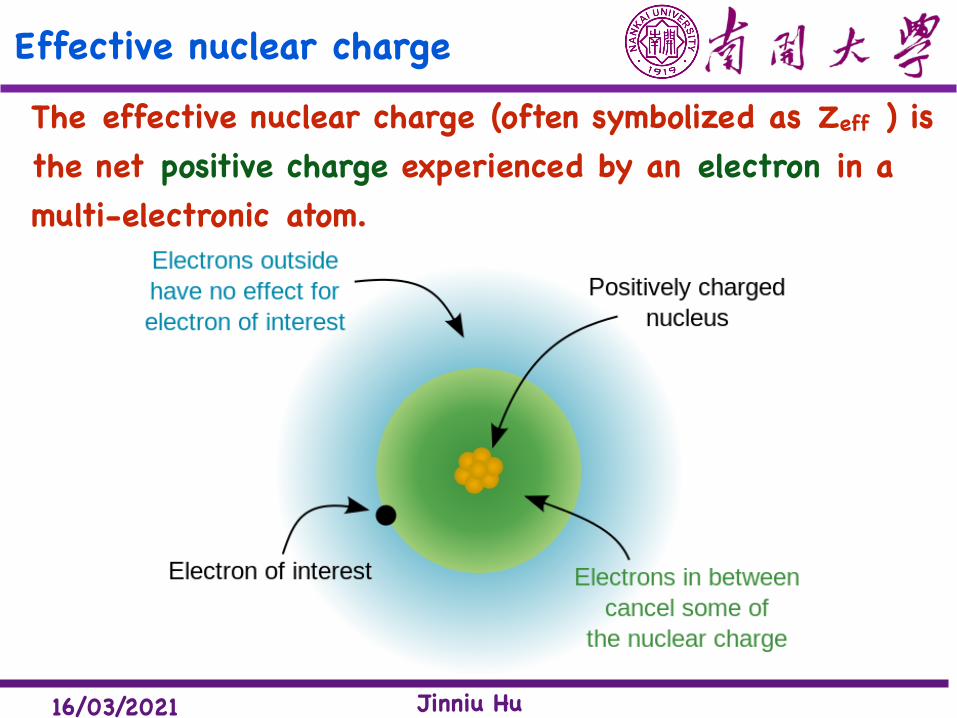
Effective nuclear chargeThe effective nuclear charge (often symbolized as Zeff ) is the net positive charge experienced by an electron in a multi-electronic atom.
16/03/2021 Jinniu Hu
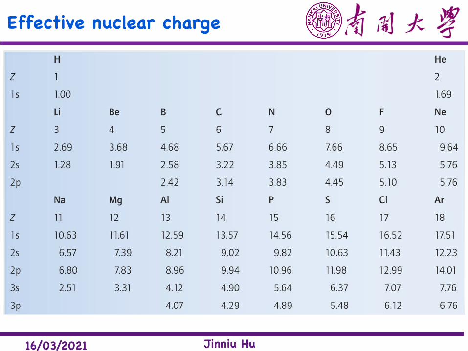
Effective nuclear charge
16/03/2021 Jinniu Hu
Heart curve
16/03/2021 Jinniu Hu
Homework
The Physics of Atoms and Quanta
8.1, 8.2, 8.3, 8.6, 8.8, 8.18
23/03/2021 Jinniu Hu
Exercise class 1.Determine the longest and shortest wavelengths observed in the Paschen series for hydrogen. Which are visible?
23/03/2021 Jinniu Hu
Exercise class 1.Determine the longest and shortest wavelengths observed in the Paschen series for hydrogen. Which are visible?
Solution: We insert the values of n into Rydberg equation to obtain
1
�max= (1.0974⇥ 107)
✓1
32� 1
42
◆= 5.335⇥ 105 m�1
�max = 1875 nm
and 1
�min= (1.0974⇥ 107)
✓1
32� 1
12
◆= 1.219⇥ 106 m�1
�min = 820 nmThe minimum and maximum wavelengths are both not visible and are both in the infrared.
23/03/2021 Jinniu Hu
Exercise class 2.Calculate the wavelength for the nu=3 to nl=2 transition (called the H$ line) for the atoms of hydrogen, deuterium, and tritium.
23/03/2021 Jinniu Hu
Exercise class 2.Calculate the wavelength for the nu=3 to nl=2 transition (called the H$ line) for the atoms of hydrogen, deuterium, and tritium.
4.5 Successes and Failures of the Bohr Model 149
The Bohr model may be applied to any single-electron atom (hydrogen-like) even if the nuclear charge is greater than 1 proton charge (!e), for ex-ample He! and Li!!. The only change needed is in the calculation of the Cou-lomb force, where e2 is replaced by Ze2 to account for the nuclear charge of !Ze. The Rydberg Equation (4.30) now becomes
1l
" Z 2R a 1n /
2 #1
nu2 b (4.38)
where the Rydberg constant is given by Equation (4.37). Bohr applied his model to the case of singly ionized helium, He!. We emphasize that Equation (4.38) is valid only for single-electron atoms (H, He!, Li!!, and so on) and does not ap-ply to any other atoms (for example He, Li, Li!). Charged atoms, such as He!, Li!, and Li!!, are called ions.
In his original paper of 1913, Bohr predicted the spectral lines of He! al-though they had not yet been identified in the lab. He showed that certain lines (generally ascribed to hydrogen) that had been observed by Pickering in stellar spectra, and by Fowler in vacuum tubes containing both hydrogen and helium, could be identified as singly ionized helium. Bohr showed that the wavelengths predicted for He! with n/ " 4 are almost identical to those of H for n/ " 2, ex-cept that He! has additional lines between those of H (see Problem 35). The correct explanation of this fact by Bohr gave credibility to his model.
Calculate the wavelength for the nu " 3 S n/ " 2 transition (called the Ha line) for the atoms of hydrogen, deuterium, and tritium.
Strategy We use Equation (4.30) but with R q replaced by the Rydberg constant expressed in Equation (4.37). In or-der to use Equation (4.37) we will need the masses for hy-drogen, deuterium, and tritium.
Solution The following masses are obtained by subtract-ing the electron mass from the atomic masses given in Ap-pendix 8.
Proton " 1.007276 u
Deuteron " 2.013553 u
Triton 1tritium nucleus 2 " 3.015500 u
The electron mass is me " 0.0005485799 u. The Rydberg constants are
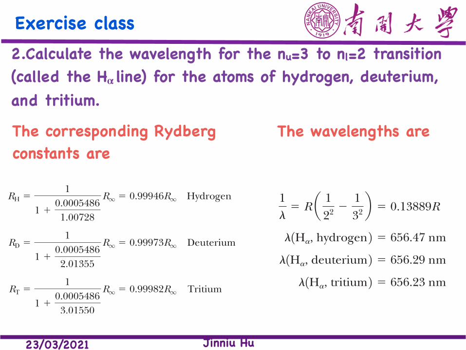
RH "1
1 !0.00054861.00728
Rq " 0.99946Rq Hydrogen
RD "1
1 !0.00054862.01355
Rq " 0.99973Rq Deuterium
RT "1
1 !0.00054863.01550
Rq " 0.99982Rq Tritium
The calculated wavelength for the Ha line is
1l
" R a 122 #
132 b " 0.13889R
l1Ha, hydrogen 2 " 656.47 nm
l1Ha, deuterium 2 " 656.29 nm
l1Ha, tritium 2 " 656.23 nm
Deuterium was discovered when two closely spaced spec-tral lines of hydrogen near 656.4 nm were observed in 1932. These proved to be the Ha lines of atomic hydrogen and deuterium.
EXAMPLE 4 .8
03721_ch04_127-161.indd 14903721_ch04_127-161.indd 149 9/29/11 9:36 AM9/29/11 9:36 AM
Solution: The masses of proton, deuteron and triton are
23/03/2021 Jinniu Hu
Exercise class 2.Calculate the wavelength for the nu=3 to nl=2 transition (called the H$ line) for the atoms of hydrogen, deuterium, and tritium.
4.5 Successes and Failures of the Bohr Model 149
The Bohr model may be applied to any single-electron atom (hydrogen-like) even if the nuclear charge is greater than 1 proton charge (!e), for ex-ample He! and Li!!. The only change needed is in the calculation of the Cou-lomb force, where e2 is replaced by Ze2 to account for the nuclear charge of !Ze. The Rydberg Equation (4.30) now becomes
1l
" Z 2R a 1n /
2 #1
nu2 b (4.38)
where the Rydberg constant is given by Equation (4.37). Bohr applied his model to the case of singly ionized helium, He!. We emphasize that Equation (4.38) is valid only for single-electron atoms (H, He!, Li!!, and so on) and does not ap-ply to any other atoms (for example He, Li, Li!). Charged atoms, such as He!, Li!, and Li!!, are called ions.
In his original paper of 1913, Bohr predicted the spectral lines of He! al-though they had not yet been identified in the lab. He showed that certain lines (generally ascribed to hydrogen) that had been observed by Pickering in stellar spectra, and by Fowler in vacuum tubes containing both hydrogen and helium, could be identified as singly ionized helium. Bohr showed that the wavelengths predicted for He! with n/ " 4 are almost identical to those of H for n/ " 2, ex-cept that He! has additional lines between those of H (see Problem 35). The correct explanation of this fact by Bohr gave credibility to his model.
Calculate the wavelength for the nu " 3 S n/ " 2 transition (called the Ha line) for the atoms of hydrogen, deuterium, and tritium.
Strategy We use Equation (4.30) but with R q replaced by the Rydberg constant expressed in Equation (4.37). In or-der to use Equation (4.37) we will need the masses for hy-drogen, deuterium, and tritium.
Solution The following masses are obtained by subtract-ing the electron mass from the atomic masses given in Ap-pendix 8.
Proton " 1.007276 u
Deuteron " 2.013553 u
Triton 1tritium nucleus 2 " 3.015500 u
The electron mass is me " 0.0005485799 u. The Rydberg constants are
RH "1
1 !0.00054861.00728
Rq " 0.99946Rq Hydrogen
RD "1
1 !0.00054862.01355
Rq " 0.99973Rq Deuterium
RT "1
1 !0.00054863.01550
Rq " 0.99982Rq Tritium
The calculated wavelength for the Ha line is
1l
" R a 122 #
132 b " 0.13889R
l1Ha, hydrogen 2 " 656.47 nm
l1Ha, deuterium 2 " 656.29 nm
l1Ha, tritium 2 " 656.23 nm
Deuterium was discovered when two closely spaced spec-tral lines of hydrogen near 656.4 nm were observed in 1932. These proved to be the Ha lines of atomic hydrogen and deuterium.
EXAMPLE 4 .8
03721_ch04_127-161.indd 14903721_ch04_127-161.indd 149 9/29/11 9:36 AM9/29/11 9:36 AM
The corresponding Rydberg constants are
4.5 Successes and Failures of the Bohr Model 149
The Bohr model may be applied to any single-electron atom (hydrogen-like) even if the nuclear charge is greater than 1 proton charge (!e), for ex-ample He! and Li!!. The only change needed is in the calculation of the Cou-lomb force, where e2 is replaced by Ze2 to account for the nuclear charge of !Ze. The Rydberg Equation (4.30) now becomes
1l
" Z 2R a 1n /
2 #1
nu2 b (4.38)
where the Rydberg constant is given by Equation (4.37). Bohr applied his model to the case of singly ionized helium, He!. We emphasize that Equation (4.38) is valid only for single-electron atoms (H, He!, Li!!, and so on) and does not ap-ply to any other atoms (for example He, Li, Li!). Charged atoms, such as He!, Li!, and Li!!, are called ions.
In his original paper of 1913, Bohr predicted the spectral lines of He! al-though they had not yet been identified in the lab. He showed that certain lines (generally ascribed to hydrogen) that had been observed by Pickering in stellar spectra, and by Fowler in vacuum tubes containing both hydrogen and helium, could be identified as singly ionized helium. Bohr showed that the wavelengths predicted for He! with n/ " 4 are almost identical to those of H for n/ " 2, ex-cept that He! has additional lines between those of H (see Problem 35). The correct explanation of this fact by Bohr gave credibility to his model.
Calculate the wavelength for the nu " 3 S n/ " 2 transition (called the Ha line) for the atoms of hydrogen, deuterium, and tritium.
Strategy We use Equation (4.30) but with R q replaced by the Rydberg constant expressed in Equation (4.37). In or-der to use Equation (4.37) we will need the masses for hy-drogen, deuterium, and tritium.
Solution The following masses are obtained by subtract-ing the electron mass from the atomic masses given in Ap-pendix 8.
Proton " 1.007276 u
Deuteron " 2.013553 u
Triton 1tritium nucleus 2 " 3.015500 u
The electron mass is me " 0.0005485799 u. The Rydberg constants are
RH "1
1 !0.00054861.00728
Rq " 0.99946Rq Hydrogen
RD "1
1 !0.00054862.01355
Rq " 0.99973Rq Deuterium
RT "1
1 !0.00054863.01550
Rq " 0.99982Rq Tritium
The calculated wavelength for the Ha line is
1l
" R a 122 #
132 b " 0.13889R
l1Ha, hydrogen 2 " 656.47 nm
l1Ha, deuterium 2 " 656.29 nm
l1Ha, tritium 2 " 656.23 nm
Deuterium was discovered when two closely spaced spec-tral lines of hydrogen near 656.4 nm were observed in 1932. These proved to be the Ha lines of atomic hydrogen and deuterium.
EXAMPLE 4 .8
03721_ch04_127-161.indd 14903721_ch04_127-161.indd 149 9/29/11 9:36 AM9/29/11 9:36 AM
The wavelengths are
23/03/2021 Jinniu Hu
Exercise class 3.Calculate the shortest wavelength that can be emitted by the Li++ ion.
23/03/2021 Jinniu Hu
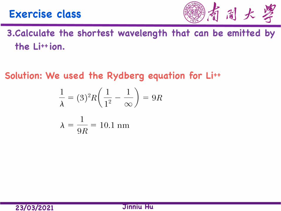
Exercise class 3.Calculate the shortest wavelength that can be emitted by the Li++ ion.
150 Chapter 4 Structure of the Atom
Other LimitationsAs the level of precision increased in optical spectrographs, it was observed that each of the lines, originally believed to be single, actually could be resolved into two or more lines, known as fi ne structure. Arnold Sommerfeld adapted the spe-cial theory of relativity (assuming some of the electron orbits were elliptical) to Bohr’s hypotheses and was able to account for some of the “splitting” of spectral lines. Subsequently it has been found that other factors (especially the electron’s spin, or intrinsic angular momentum) also affect the fine structure of spectral lines.
It was soon observed that external magnetic fields (the Zeeman effect) and external electric fields (the Stark effect) applied to the radiating atoms affected the spectral lines, splitting and broadening them. Although classical electromag-netic theory could quantitatively explain the (normal) Zeeman effect (see Chap-ter 7), it was unable to account for the Stark effect; for this the quantum model of Bohr and Sommerfeld was necessary.
Although the Bohr model was a great step forward in the application of the new quantum theory to understanding the tiny atom, it soon became apparent that the model had its limitations:
1. It could be successfully applied only to single-electron atoms (H, He!, Li!!, and so on).
2. It was not able to account for the intensities or the fine structure of the spectral lines.
3. Bohr’s model could not explain the binding of atoms into molecules.
We discuss in Chapter 7 the full quantum mechanical theory of the hydro-gen atom, which accounts for all of these phenomena. The Bohr model was an ad hoc theory to explain the hydrogen spectral lines. Although it was useful in the beginnings of quantum physics, we now know that the Bohr model does not correctly describe atoms. Despite its flaws, Bohr’s model should not be deni-grated. It was the first step from a purely classical description of the atom to the correct quantum explanation. As usually happens in such tremendous changes of understanding, Bohr’s model simply did not go far enough—he retained too many classical concepts. Einstein, many years later, noted* that Bohr’s achieve-ment “appeared to me like a miracle and appears as a miracle even today.”
Fine structure
Limitations of Bohr model
Calculate the shortest wavelength that can be emitted by the Li!! ion.
Strategy The shortest wavelength occurs when the elec-tron changes from the highest state (unbound, nu " q) to the lowest state (n/ " 1). We use Equation (4.38) to calcu-late the wavelength.
Solution Equation (4.38) gives
1l
" 13 22R a 112 #
1q b " 9R
l "1
9R" 10.1 nm
When we let nu " q, we have what is known as the series limit, which is the shortest wavelength possibly emitted for each of the named series.
EXAMPLE 4 .9
*P. A. Schillp, ed., Albert Einstein, Philosopher-Scientist, La Salle, IL: The Open Court, 1949.
03721_ch04_127-161.indd 15003721_ch04_127-161.indd 150 9/29/11 9:36 AM9/29/11 9:36 AM
Solution: We used the Rydberg equation for Li++
23/03/2021 Jinniu Hu
Exercise class 4. An atom with one electron has the energy levels En =−a/
n2 . Its spectrum has two neighboring lines with �1= 97.5nm and �2 = 102.8nm in Lyman series. What is the value of the constant a and which atomic element belongs to this spectrum?
23/03/2021 Jinniu Hu
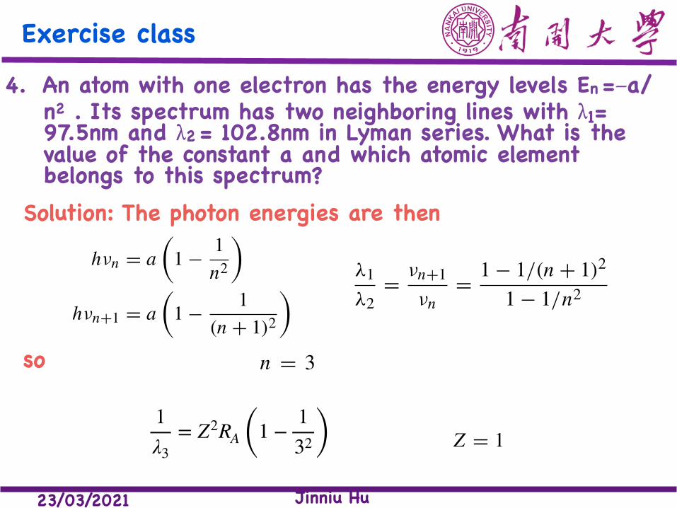
Exercise class 4. An atom with one electron has the energy levels En =−a/
n2 . Its spectrum has two neighboring lines with �1= 97.5nm and �2 = 102.8nm in Lyman series. What is the value of the constant a and which atomic element belongs to this spectrum?
Solution: The photon energies are then
502 Solutions to the Exercises
c) The relativistic mass increase is
∆m = m − m0 = m0
(1
√1 − v2/c2
− 1
)
= m0
(1√
1 − 0.5172− 1
)
= 0.17m0.
The relativistic energy correction is (see Sect. 5.4)
∆Er(n = 1, Z = 1) = 9 × 10⁻⁴ eV.
For Z = 79 it is
∆Er(n = 1, Z = 79) = 5.6 eV.
7. After the mean life time τ the number of neutrons havedecayed to 1/e of the initial value and after the time τ ln 2to 1/2 of the initial value. During this time they travel adistance x = vτ ln 2.The velocity of the neutrons is
v = hmλ
⇒ x = hτ ln 2mλ
= 6.62 × 10−34 × 900 × 0.691.67 × 10−27 × 10−9 = 2.4 × 10⁵ m.
The decay time of the neutrons could be measured bytrapping them in a magnetic quadrupole trap with thegeometry of a circle. With a radius r = 1m, they travel(2.4×10⁵/2π) = 4×10⁴ times around the circle beforethey decay, if no other losses are present.
8. Thewavelength of the Lyman α-line can be obtained fromthe relation
hν = hcλ
= Ry∗(1 − 1
4
)
⇒ λ = 43 Ry
with Ry = Ry∗/hc.
a)
Ry(3H)= Ry∞ · µ
mewith µ = memN
me + mN,
where mN is the mass of the nucleus.
⇒ Ry(3H)= Ry∞
11+ me/mN
≈ Ry∞1
1+ 13·1836
= 0.999818Ry∞
= 1.0971738 × 10⁷ m−1.
The wavelength of Lyman α n = 2 → n = 1 is then:
λ = 43Ry
= 1.215 × 10⁻⁷ m = 121.5 nm
b) For positronium (e+e−)
µ = me/2 ⇒ Ry(e−e+) = 12Ry∞
⇒ λ = 243.0 nm.
9. At room temperature (T = 300K) only the ground stateis populated.Therefore all absorbing transitions start fromthe ground state with n = 1. The photon energies are then
hνn = a(1 − 1
n2
)
hνn+1 = a(1 − 1
(n + 1)2
)
with λ = c/ν we obtain
λ1
λ2= νn+1
νn= 1 − 1/(n + 1)2
1 − 1/n2.
With λ1 = 97.5nm, λ2 = 102.8 nm ⇒ λ1/λ2 = 0.948.For n = 2 ⇒ λ1/λ2 = 0.843, for n = 3 ⇒ λ1/λ2 =0.948.The two lines therefore belong to n = 3 and n = 4. Theconstant a can be determined from
νn = cλn
= ah
(1 − 1
n2
)
with λ3 = 102.8nm we obtain
a = hcλ3
11 − 1/32
= hcλ3
· 98= 2.177 × 10⁻¹⁸ J = Ry∗.
The lines therefore belong to transitions in the hydrogenatom with Z = 1, n = 3 and n = 4.
10. Since the resolving power of the spectrograph is assumedto be
∣∣∣∣λ
∆λ
∣∣∣∣ =∣∣∣
ν
∆ν
∣∣∣ = 5 × 10⁵
the difference ∆ν of two adjacent lines in the Balmerspectrum has to be ∆ν ≥ ν/(5 × 105). The frequenciesof the Balmer series are
νn = Ry∗
h
(122
− 1n2
)n ≥ 3.
so
1λ3
= Z2RA (1 − 132 )
502 Solutions to the Exercises
c) The relativistic mass increase is
∆m = m − m0 = m0
(1
√1 − v2/c2
− 1
)
= m0
(1√
1 − 0.5172− 1
)
= 0.17m0.
The relativistic energy correction is (see Sect. 5.4)
∆Er(n = 1, Z = 1) = 9 × 10⁻⁴ eV.
For Z = 79 it is
∆Er(n = 1, Z = 79) = 5.6 eV.
7. After the mean life time τ the number of neutrons havedecayed to 1/e of the initial value and after the time τ ln 2to 1/2 of the initial value. During this time they travel adistance x = vτ ln 2.The velocity of the neutrons is
v = hmλ
⇒ x = hτ ln 2mλ
= 6.62 × 10−34 × 900 × 0.691.67 × 10−27 × 10−9 = 2.4 × 10⁵ m.
The decay time of the neutrons could be measured bytrapping them in a magnetic quadrupole trap with thegeometry of a circle. With a radius r = 1m, they travel(2.4×10⁵/2π) = 4×10⁴ times around the circle beforethey decay, if no other losses are present.
8. Thewavelength of the Lyman α-line can be obtained fromthe relation
hν = hcλ
= Ry∗(1 − 1
4
)
⇒ λ = 43 Ry
with Ry = Ry∗/hc.
a)
Ry(3H)= Ry∞ · µ
mewith µ = memN
me + mN,
where mN is the mass of the nucleus.
⇒ Ry(3H)= Ry∞
11+ me/mN
≈ Ry∞1
1+ 13·1836
= 0.999818Ry∞
= 1.0971738 × 10⁷ m−1.
The wavelength of Lyman α n = 2 → n = 1 is then:
λ = 43Ry
= 1.215 × 10⁻⁷ m = 121.5 nm
b) For positronium (e+e−)
µ = me/2 ⇒ Ry(e−e+) = 12Ry∞
⇒ λ = 243.0 nm.
9. At room temperature (T = 300K) only the ground stateis populated.Therefore all absorbing transitions start fromthe ground state with n = 1. The photon energies are then
hνn = a(1 − 1
n2
)
hνn+1 = a(1 − 1
(n + 1)2
)
with λ = c/ν we obtain
λ1
λ2= νn+1
νn= 1 − 1/(n + 1)2
1 − 1/n2.
With λ1 = 97.5nm, λ2 = 102.8 nm ⇒ λ1/λ2 = 0.948.For n = 2 ⇒ λ1/λ2 = 0.843, for n = 3 ⇒ λ1/λ2 =0.948.The two lines therefore belong to n = 3 and n = 4. Theconstant a can be determined from
νn = cλn
= ah
(1 − 1
n2
)
with λ3 = 102.8nm we obtain
a = hcλ3
11 − 1/32
= hcλ3
· 98= 2.177 × 10⁻¹⁸ J = Ry∗.
The lines therefore belong to transitions in the hydrogenatom with Z = 1, n = 3 and n = 4.
10. Since the resolving power of the spectrograph is assumedto be
∣∣∣∣λ
∆λ
∣∣∣∣ =∣∣∣
ν
∆ν
∣∣∣ = 5 × 10⁵
the difference ∆ν of two adjacent lines in the Balmerspectrum has to be ∆ν ≥ ν/(5 × 105). The frequenciesof the Balmer series are
νn = Ry∗
h
(122
− 1n2
)n ≥ 3.