Embed Size (px)
Citation preview

Comp. Graphics (U), Chap 2 Global View 1 CGGM Lab., CS Dept., NCTU Jung Hong Chuang
Chapter 2
A top-down approach -How to make shaded images?

Comp. Graphics (U), Chap 2 Global View 2 CGGM Lab., CS Dept., NCTU Jung Hong Chuang
Graphics API vs. application API
• Graphics API – Support rendering pipeline for polygon stream– Pipeline process supported by graphics hardware – Examples
• OpenGL, Direct 3D
• Application API– A software engine that calls graphics API for rendering a
scene• Scene management, real-time rendering, animation
modules,…
– Home made programs vs. programming using application API• Either one will call graphics API for rendering polygons
– Examples• OpenInventer, WTK, Unreal3 (game engine), Ogre, Utility….

Comp. Graphics (U), Chap 2 Global View 3 CGGM Lab., CS Dept., NCTU Jung Hong Chuang
How to make shaded images?Rendering Pipeline

Comp. Graphics (U), Chap 2 Global View 4 CGGM Lab., CS Dept., NCTU Jung Hong Chuang
How to make shaded images?Input
• Set up scene, light, viewing data
– Object geometry and material
• Geometry: Primitives, ex., polygon meshes
– vertex attributes
» Coordinates, normal, color, and texture coordinates
• Texture maps for material and others
– Color map, normal map, bump map, displacement map, light map, environment map,…
– Lighting information
• Light setting, light control parameters
– Viewing information and view volume
• Eye point, view direction/orientation, view window/volume

Comp. Graphics (U), Chap 2 Global View 5 CGGM Lab., CS Dept., NCTU Jung Hong Chuang
Rendering Pipeline
• Per-vertex operations
View transformation/lighting stage– Apply viewing transformation to transform
polygon vertices to view coordinate system and ten do the projection
– Transform vertex normal
– Compute lighting (Phong model) at each vertex in view coordinate system
– Generate (if necessary) and transform texture coordinates

Comp. Graphics (U), Chap 2 Global View 6 CGGM Lab., CS Dept., NCTU Jung Hong Chuang
Rendering Pipeline
• Primitive assembly– Input to the pipeline – vertices
– Assemble vertices to primitives• Polygon, triangle, polyline

Comp. Graphics (U), Chap 2 Global View 7 CGGM Lab., CS Dept., NCTU Jung Hong Chuang
Rendering Pipeline
• Clipping– Clip the triangle against the normalized view
volume
– Back-face culling
– Perspective division
Comp. Graphics (U), Chap 2 Global View 8 CGGM Lab., CS Dept., NCTU Jung Hong Chuang
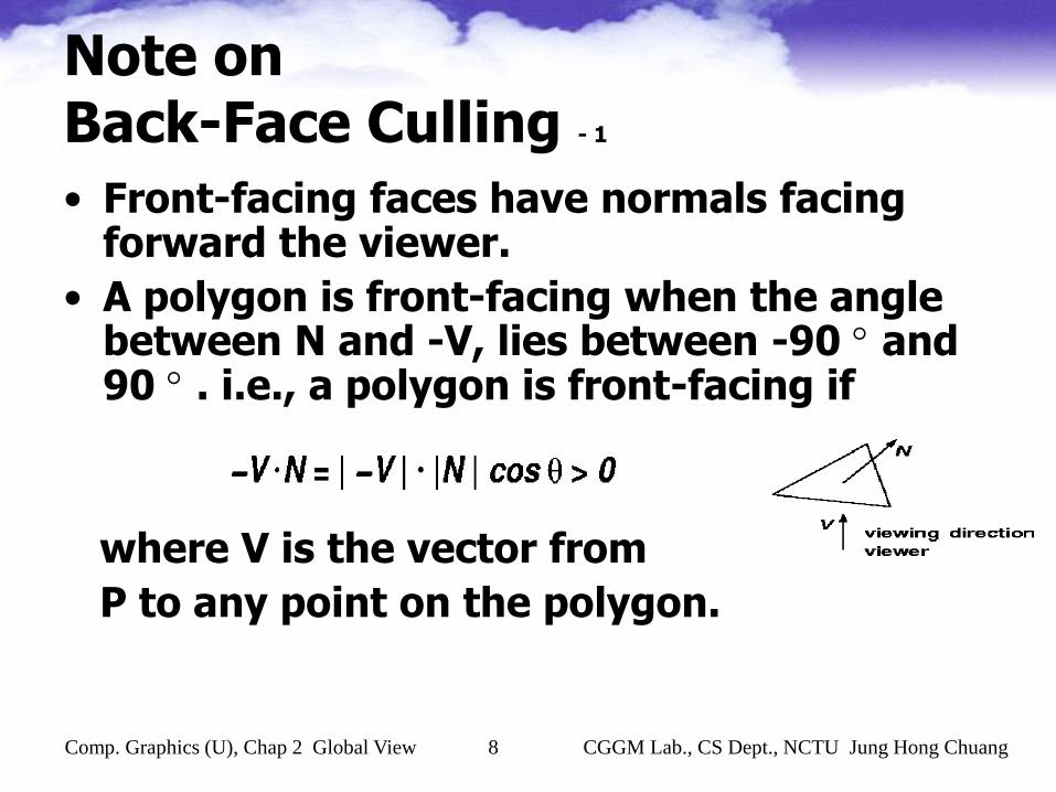
Note onBack-Face Culling - 1
• Front-facing faces have normals facing forward the viewer.
• A polygon is front-facing when the angle between N and -V, lies between -90 and 90 . i.e., a polygon is front-facing if
where V is the vector from
P to any point on the polygon.
Comp. Graphics (U), Chap 2 Global View 9 CGGM Lab., CS Dept., NCTU Jung Hong Chuang
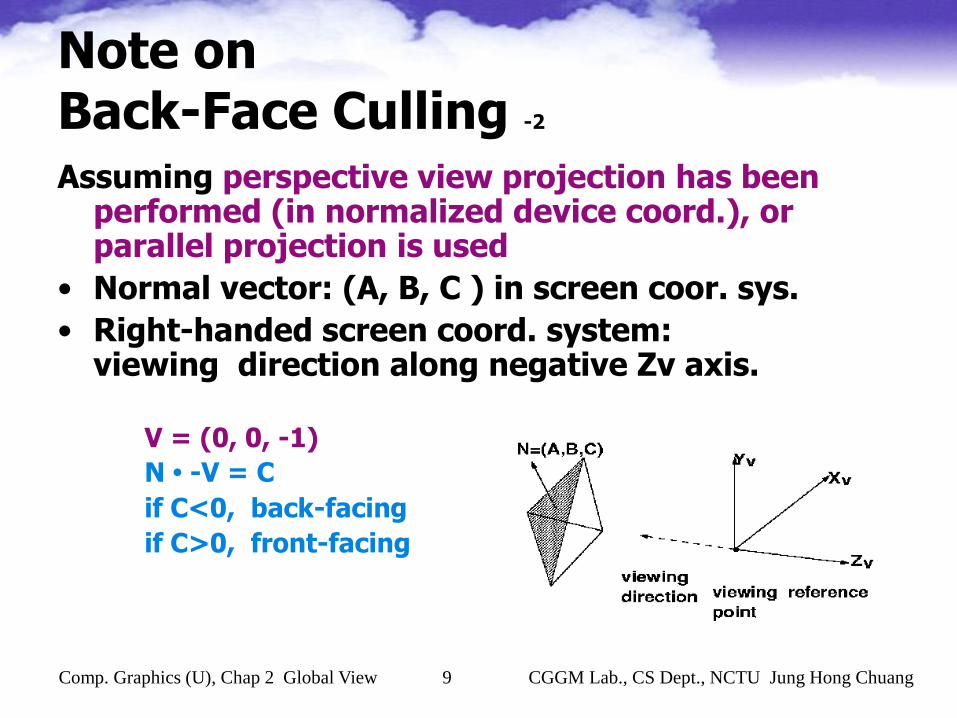
Note onBack-Face Culling -2
Assuming perspective view projection has been performed (in normalized device coord.), or parallel projection is used
• Normal vector: (A, B, C ) in screen coor. sys.
• Right-handed screen coord. system: viewing direction along negative Zv axis.
V = (0, 0, -1)
N • -V = C
if C<0, back-facing
if C>0, front-facing

Comp. Graphics (U), Chap 2 Global View 10 CGGM Lab., CS Dept., NCTU Jung Hong Chuang
Note onBack-Face Culling - 3
• Left handed screen coor. system:
Viewing direction along the positive Zv direction
Comp. Graphics (U), Chap 2 Global View 11 CGGM Lab., CS Dept., NCTU Jung Hong Chuang
Rendering Pipeline
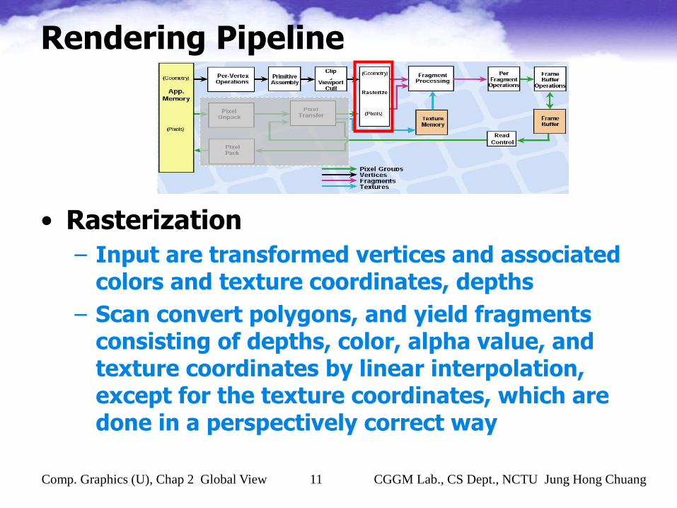
• Rasterization
– Input are transformed vertices and associated colors and texture coordinates, depths
– Scan convert polygons, and yield fragments consisting of depths, color, alpha value, and texture coordinates by linear interpolation, except for the texture coordinates, which are done in a perspectively correct way

Comp. Graphics (U), Chap 2 Global View 12 CGGM Lab., CS Dept., NCTU Jung Hong Chuang
Rendering Pipeline
Comp. Graphics (U), Chap 2 Global View 13 CGGM Lab., CS Dept., NCTU Jung Hong Chuang
Rendering Pipeline
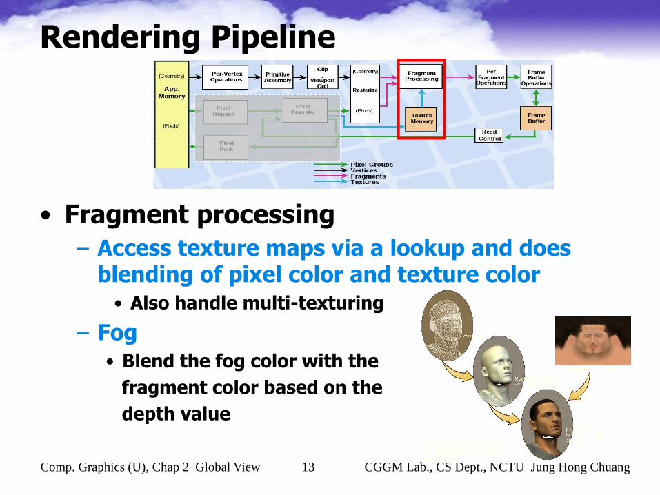
• Fragment processing
– Access texture maps via a lookup and does blending of pixel color and texture color
• Also handle multi-texturing
– Fog
• Blend the fog color with the
fragment color based on the
depth value

Comp. Graphics (U), Chap 2 Global View 14 CGGM Lab., CS Dept., NCTU Jung Hong Chuang
Rendering Pipeline
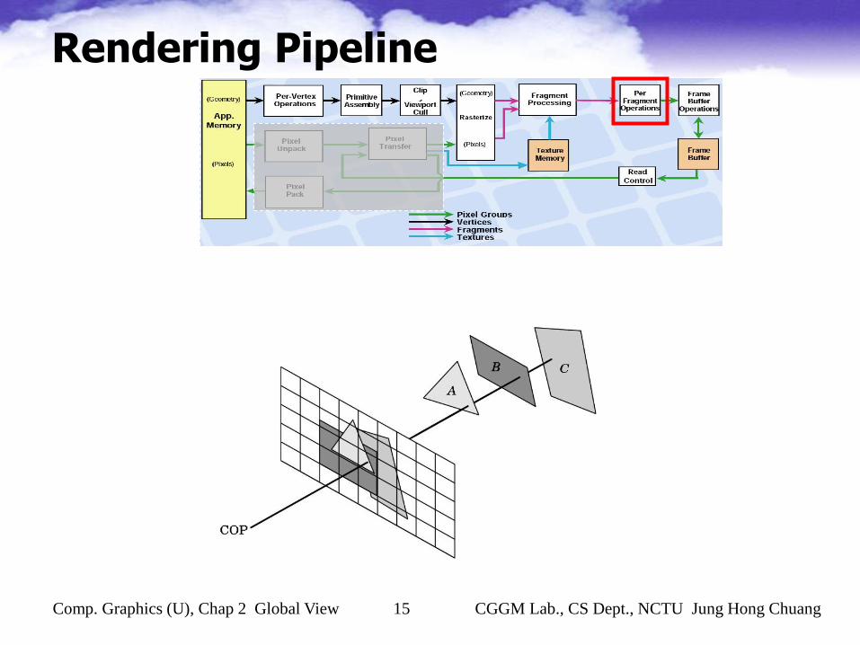
• Per-fragment operations– Alpha test (compare with alpha, keep or drop it) and
Alpha blending
– Stencil test (mask the fragment depending on the content of the stencil buffer)
– Depth test (z buffer algorithm)
– Dithering (make the color look better for low res display mode)
– Fragments passing all tests are written to frame-buffer
Comp. Graphics (U), Chap 2 Global View 15 CGGM Lab., CS Dept., NCTU Jung Hong Chuang
Rendering Pipeline

Comp. Graphics (U), Chap 2 Global View 16 CGGM Lab., CS Dept., NCTU Jung Hong Chuang
Rendering Pipeline
• Frame-buffer operations
– Operations performed on the whole frame buffer
• Accumulation buffer operations for multipass rendering

Comp. Graphics (U), Chap 2 Global View 17 CGGM Lab., CS Dept., NCTU Jung Hong Chuang
OpenGL Viewing Pipeline -1
View transform
Viewing projection
View-Volume Clipping
Back-face culling
Window-viewportmapping

Comp. Graphics (U), Chap 2 Global View 18 CGGM Lab., CS Dept., NCTU Jung Hong Chuang
OpenGL Viewing Pipeline -2

Comp. Graphics (U), Chap 2 Global View 19 CGGM Lab., CS Dept., NCTU Jung Hong Chuang
Viewing Pipeline -1
• View transformation – Transformation objects from world coordinate
system to the view coordinate system• For fast perspective projection
• Involves translation and rotation
• View projection – Transforms the view volume to a normalized
view volume and does the orthogonal projection.• Easy for hardware 3-D clipping
• Any projection becomes orthogonal projection
• Clipping can be unified for perspective and parallel projection
• Involves translation, shearing, and scaling

Comp. Graphics (U), Chap 2 Global View 20 CGGM Lab., CS Dept., NCTU Jung Hong Chuang
Viewing Pipeline - 2
View Transformation

Comp. Graphics (U), Chap 2 Global View 21 CGGM Lab., CS Dept., NCTU Jung Hong Chuang
Viewing Pipeline - 3
View Projection
View-volume culling w.r.t. view volume in world/eye space

Comp. Graphics (U), Chap 2 Global View 22 CGGM Lab., CS Dept., NCTU Jung Hong Chuang
Viewing Pipeline - 4
View Projection
Converting view frustum to normalized view volume

Comp. Graphics (U), Chap 2 Global View 23 CGGM Lab., CS Dept., NCTU Jung Hong Chuang
Viewing Pipeline - 4
View Projection
• Converting view frustum to normalized view volume ensures
– Any type of projection becomes orthographic projection
• Distort the objects and the do the orthogonal projection
• Orthographic projection of the distorted objects
= the projection of the original object
– Preserves depth ordering
Comp. Graphics (U), Chap 2 Global View 24 CGGM Lab., CS Dept., NCTU Jung Hong Chuang
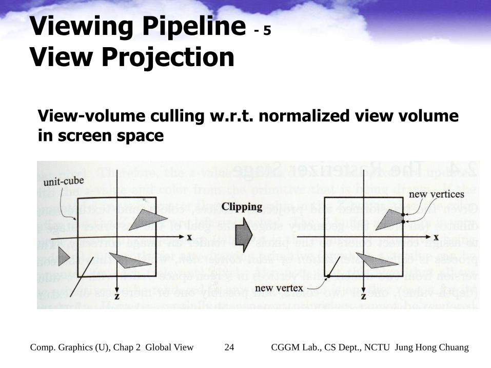
Viewing Pipeline - 5
View Projection
View-volume culling w.r.t. normalized view volume in screen space
Comp. Graphics (U), Chap 2 Global View 25 CGGM Lab., CS Dept., NCTU Jung Hong Chuang
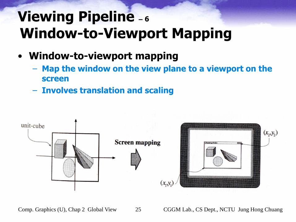
Viewing Pipeline – 6
Window-to-Viewport Mapping
• Window-to-viewport mapping
– Map the window on the view plane to a viewport on the screen
– Involves translation and scaling

Comp. Graphics (U), Chap 2 Global View 26 CGGM Lab., CS Dept., NCTU Jung Hong Chuang
3-D Geometric Transformations
• Building up a scene using 3-D transformation to instance objects
– For a complex object or scene, each subpart may have their own local coordinate systems.
– Instancing a subpart by transforming the local coordinate system by a series or translations, scalings, and rotations
• Projecting 3D objects onto a 2D view plane
– Involves scaling, translation, rotation, and shearing

Comp. Graphics (U), Chap 2 Global View 27 CGGM Lab., CS Dept., NCTU Jung Hong Chuang
Scene/Object Instancing

Comp. Graphics (U), Chap 2 Global View 28 CGGM Lab., CS Dept., NCTU Jung Hong Chuang
Translation
• Translation– Displaces points by a fixed distance in a given
direction, specified by a displacement vector.
– A rigid-body transformation
– The definition makes no reference to a frame.
– The matrix has 3 degrees of freedom for specifying the displacement vector
Matrix form in 3D? No.
It is not linear, but affine
Comp. Graphics (U), Chap 2 Global View 29 CGGM Lab., CS Dept., NCTU Jung Hong Chuang
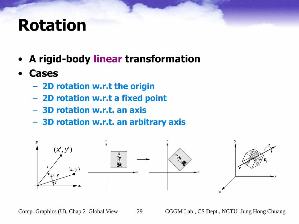
Rotation
• A rigid-body linear transformation
• Cases
– 2D rotation w.r.t the origin
– 2D rotation w.r.t a fixed point
– 3D rotation w.r.t. an axis
– 3D rotation w.r.t. an arbitrary axis
)','( yx

Comp. Graphics (U), Chap 2 Global View 30 CGGM Lab., CS Dept., NCTU Jung Hong Chuang
Scaling
• A non-rigid-body linear transformation
• To specify a scaling, we need to specify a fixed point and a direction in which we wish to scale, and a scale factor
• Negative value of gives us reflection.

Comp. Graphics (U), Chap 2 Global View 31 CGGM Lab., CS Dept., NCTU Jung Hong Chuang
Shearing
• A non-rigid-body linear transformation.
• Shear in one axis direction, others unchanged
• Example: shear in x-direction
zz
yy
yxx
'
'
cot'
)','( yx
θ

Comp. Graphics (U), Chap 2 Global View 32 CGGM Lab., CS Dept., NCTU Jung Hong Chuang
Affine transformation -1
• Linear transformation
• Affine transformation
– Preserving affine combinations of points
• Interior points of a line will be linear combination of the transformations of vertices
– So what we must deal with are vertices
– Preserve lines and parallelism of lines, but not lengths and angles. Examples:
• Rotation, scaling, shearing, translation
• Rotating a unit cube by a degree and scale in x, not in y
LXX '
bLXX '

Comp. Graphics (U), Chap 2 Global View 33 CGGM Lab., CS Dept., NCTU Jung Hong Chuang
Affine transformation -2
Preserves affine combinations/lines
)()1()(
])()[1(])([
)]1([)()1()(
])1([))((
)()1()())1(( :Claim
:ation transformAffine
,:points Two
10
10
10
10
1010
10
PAPA
bPLbPL
bPLPL
bPPLPA
PAPAPPA
bLxA
PP
Preserves relative ratios too!!

Comp. Graphics (U), Chap 2 Global View 34 CGGM Lab., CS Dept., NCTU Jung Hong Chuang
Affine transformation -2
Preserving affine combinations
Preserves relative ratios!!

Comp. Graphics (U), Chap 2 Global View 35 CGGM Lab., CS Dept., NCTU Jung Hong Chuang
Affine transformation -3
Preserving parallelism of lines
!!or on t independen vector,direction a is )( where
)()())((
)()(
)(])([
)(
)())((
))((//))(( :Claim
:ation transformAffine
)( // )( :Lines
00
0
0
0
0
0
00
QPvL
vLQAQA
vLPA
vLbPL
bvPL
vPAPA
QAPA
bLxA
vQQvPP

Comp. Graphics (U), Chap 2 Global View 36 CGGM Lab., CS Dept., NCTU Jung Hong Chuang
Homogeneous Coordinates -1
• We need a uniform matrix representationso that matrix concatenation can represent a series of affine transformations using a single matrix
• Converting from Cartesian space to the homogeneous space
Mapping (x, y, z) (X, Y, Z, W) by
x = X/W, y = Y/W, z = Z/W, W 0
Comp. Graphics (U), Chap 2 Global View 37 CGGM Lab., CS Dept., NCTU Jung Hong Chuang
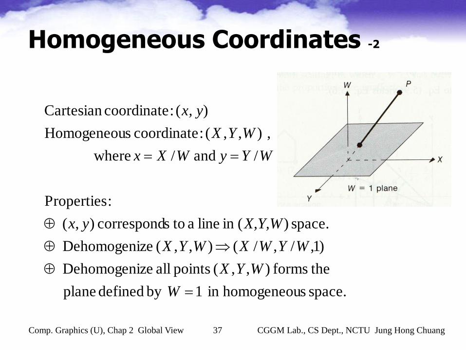
Homogeneous Coordinates -2
space. shomogeneouin 1by defined plane
theforms ),,( points all zeDehomogeni
)1,/,/( ),,( zeDehomogeni
space. )(in line a toscorrespond ),(
:Properties
/ and / where
,),,( :coordinate sHomogeneou
)( :coordinateCartesian
W
WYX
WYWXWYX
X,Y,Wyx
WYyWXx
WYX
x, y

Comp. Graphics (U), Chap 2 Global View 38 CGGM Lab., CS Dept., NCTU Jung Hong Chuang
Homogeneous Coordinates -3
• An affine transformation A can be represented in homogeneous space as a 4x4 matrix
– This transformation has 12 degrees of freedom
11000
)(
1
'
'
'
3333231
2232221
1131211
z
y
x
b
b
b
bxLxAz
y
x

Comp. Graphics (U), Chap 2 Global View 39 CGGM Lab., CS Dept., NCTU Jung Hong Chuang
Transformation in homogeneous coordinates -1
• Translation: p’=T p
• Scaling: p’=S p
1000
100
010
001
),,(z
y
x
zyxT
1000
000
000
000
),,(y
y
x
zyxS

Comp. Graphics (U), Chap 2 Global View 40 CGGM Lab., CS Dept., NCTU Jung Hong Chuang
Transformation in homogeneous coordinates -2
• Rotation: p’=Rz p
• Shearing: p’=H p
1000
0100
00cossin
00sincos
)(
zR
1000
0100
0010
00cot1
)(
xH

Comp. Graphics (U), Chap 2 Global View 41 CGGM Lab., CS Dept., NCTU Jung Hong Chuang
Concatenation of transformations -1
• q =CBAp = C(B(Ap))=Mp, where M=CBA
• Examples
– Rotation about a fixed point
– General rotation about the origin
– Rotation about an arbitrary axis

Comp. Graphics (U), Chap 2 Global View 42 CGGM Lab., CS Dept., NCTU Jung Hong Chuang
Concatenation of transformations -2
• Rotation about a fixed point
– A cube with its center p and its sides aligned with the axes. Rotate it about z-axis, about its center.
– M=T(p)Rz(theta)T(-p)

Comp. Graphics (U), Chap 2 Global View 43 CGGM Lab., CS Dept., NCTU Jung Hong Chuang
Concatenation of transformations -3
• Rotation about the origin– A cube with its center p at the origin and its
sides aligned with the axes.
– R=Rx Ry Rz

Comp. Graphics (U), Chap 2 Global View 44 CGGM Lab., CS Dept., NCTU Jung Hong Chuang
Concatenation of transformations -4
• Rotation about an arbitrary point and line
– Move the fixed point to origin
– Rotate such that the vector is coincident to z-axis
– Rotate about z-axis
)()()()()()()( 00 pTRRRRRpTM xxyyzyyxx

Comp. Graphics (U), Chap 2 Global View 45 CGGM Lab., CS Dept., NCTU Jung Hong Chuang
Projections
• Parallel projection
• Perspective projection

Comp. Graphics (U), Chap 2 Global View 46 CGGM Lab., CS Dept., NCTU Jung Hong Chuang
ProjectionsParallel projection

Comp. Graphics (U), Chap 2 Global View 47 CGGM Lab., CS Dept., NCTU Jung Hong Chuang
ProjectionsParallel projection
Comp. Graphics (U), Chap 2 Global View 48 CGGM Lab., CS Dept., NCTU Jung Hong Chuang
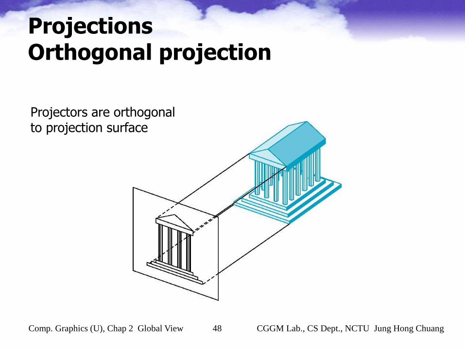
ProjectionsOrthogonal projection
Projectors are orthogonal to projection surface

Comp. Graphics (U), Chap 2 Global View 49 CGGM Lab., CS Dept., NCTU Jung Hong Chuang
ProjectionsOblique projection
Arbitrary relationship between projectors and projection plane

Comp. Graphics (U), Chap 2 Global View 50 CGGM Lab., CS Dept., NCTU Jung Hong Chuang
ProjectionPerspective Projections

Comp. Graphics (U), Chap 2 Global View 51 CGGM Lab., CS Dept., NCTU Jung Hong Chuang
ProjectionsPerspective projection

Comp. Graphics (U), Chap 2 Global View 52 CGGM Lab., CS Dept., NCTU Jung Hong Chuang
ProjectionsPerspective projection

Comp. Graphics (U), Chap 2 Global View 53 CGGM Lab., CS Dept., NCTU Jung Hong Chuang
A Practical Viewing System
• Users specify
– Projection type
– A camera position C and a viewing directionvector N (= view plane normal ), and an upvector V
– A view plane distance d , near clipping plane distance n, and a far clipping plane distance f.
– A view window is specified but it is symmetrically disposed about the center of the view plane

Comp. Graphics (U), Chap 2 Global View 54 CGGM Lab., CS Dept., NCTU Jung Hong Chuang
Viewing Parameters
World coordinate system
View coordinate system
Here without near and far clipping planes

Comp. Graphics (U), Chap 2 Global View 55 CGGM Lab., CS Dept., NCTU Jung Hong Chuang
Perspective view volume
Far

Comp. Graphics (U), Chap 2 Global View 56 CGGM Lab., CS Dept., NCTU Jung Hong Chuang
Parallel view volume
FarNear

Comp. Graphics (U), Chap 2 Global View 57 CGGM Lab., CS Dept., NCTU Jung Hong Chuang
View coordinate system
• View coordinate system (u, v, n)
– v=V, n=-N, u=v x n, where V is perpendicular to n

Comp. Graphics (U), Chap 2 Global View 58 CGGM Lab., CS Dept., NCTU Jung Hong Chuang
Viewing Pipeline
• View transformation: Tview
– world coord. sys. → view coord. sys.
– Tview = B T
– For simpler and faster clipping and projection
• View projection: Tp
– view coord. sys. → screen coord. sys.
– Convert view volume to normalized view volume and then do orthogonal projection.
– Tp = Tpers2 Tpers1

Comp. Graphics (U), Chap 2 Global View 59 CGGM Lab., CS Dept., NCTU Jung Hong Chuang
View Transformation
• View transform matrix Tview
[ xv, yv, zv, 1] = Tview [xw, yw, zw, 1]T
• Tview can be written as Tview = B T ,
where
– T translates the world coordinate origin to C.
– B rotates any vector expressed in the world coordinate system into the view coordinate system by mapping (u, v, n) to (e1,e2,e3).

Comp. Graphics (U), Chap 2 Global View 60 CGGM Lab., CS Dept., NCTU Jung Hong Chuang
View Projection -1
View volume Normalized view volume

Comp. Graphics (U), Chap 2 Global View 61 CGGM Lab., CS Dept., NCTU Jung Hong Chuang
View Projection -2
-1
View volume Normalized view volume
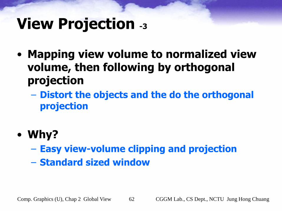
View Projection -3
• Mapping view volume to normalized view volume, then following by orthogonal projection
– Distort the objects and the do the orthogonal projection
• Why?
– Easy view-volume clipping and projection
– Standard sized window
Comp. Graphics (U), Chap 2 Global View 62 CGGM Lab., CS Dept., NCTU Jung Hong Chuang

Comp. Graphics (U), Chap 2 Global View 63 CGGM Lab., CS Dept., NCTU Jung Hong Chuang
Viewing Pipeline Summary
View transform
Viewprojection
V-V clippingin homogeneousspace
Window-Viewportmapping

Comp. Graphics (U), Chap 2 Global View 64 CGGM Lab., CS Dept., NCTU Jung Hong Chuang
Lighting Effects -1
• Lighting effects involve
– light propagation
– Light-material interaction • The interaction of light with a surface, in terms of the surface
properties and the nature of the incident light.
• Computing lighting effects in OpenGL fixed pipeline
– Vertex-lighting + Polygonal shading
• Some remarks
– Local illumination vs. global illumination.
– Polygonal shading vs. Per-pixel lighting
For lighting effect/shading, see Chap 5 of Angel’s book (6th ed.)

Comp. Graphics (U), Chap 2 Global View 65 CGGM Lab., CS Dept., NCTU Jung Hong Chuang
Lighting Effects -2
• Local lighting
– Consider lights that directly come from the light sources
• The light-surface interaction depend on only the surface material properties, surface’s local geometry,
and parameters of the light sources
– Can be added to a fast pipeline graphics architecture
• Global lighting
– Lighting is a recursive process and amounts to an integral equation (the rendering equation)
– Approximations: ray tracing and radiosity

Comp. Graphics (U), Chap 2 Global View 66 CGGM Lab., CS Dept., NCTU Jung Hong Chuang
Light Sources -1
• Light source
– An object that emits light only through internal sources
• Illumination function
– Each point (x,y,z) on the surface of the light source can emit light that is characterized by
• : the direction of emission
• : wavelength
),,,,,( zyxI
),(

Comp. Graphics (U), Chap 2 Global View 67 CGGM Lab., CS Dept., NCTU Jung Hong Chuang
Light Sources -2
• On a surface point that is illuminated
– Total contribution of the source is obtained by integrating over the surface of the source.
– The calculation is difficult for a distributed light source.

Comp. Graphics (U), Chap 2 Global View 68 CGGM Lab., CS Dept., NCTU Jung Hong Chuang
Light Sources -3
• Four types of light source
– Ambient lighting
• Provides a uniform light level in the scene.
• Can be characterized by a constant intensity Ia=[Iar, Iag, Iab]
• Each surface can reflect this light differently.
– Point light sources
– Spotlights
– Distant light

Comp. Graphics (U), Chap 2 Global View 69 CGGM Lab., CS Dept., NCTU Jung Hong Chuang
Light Sources -4
• Point light sources
– An ideal point source emits light equally in all directions.
– A point source at p0 can be characterized by
– At a surface point p, the intensity of light received from the point source is
)(
)(
)(
)(
0
0
0
0
pI
pI
pI
pI
b
g
r
)(1
),( 02
0
0 pIpp
ppI
Comp. Graphics (U), Chap 2 Global View 70 CGGM Lab., CS Dept., NCTU Jung Hong Chuang
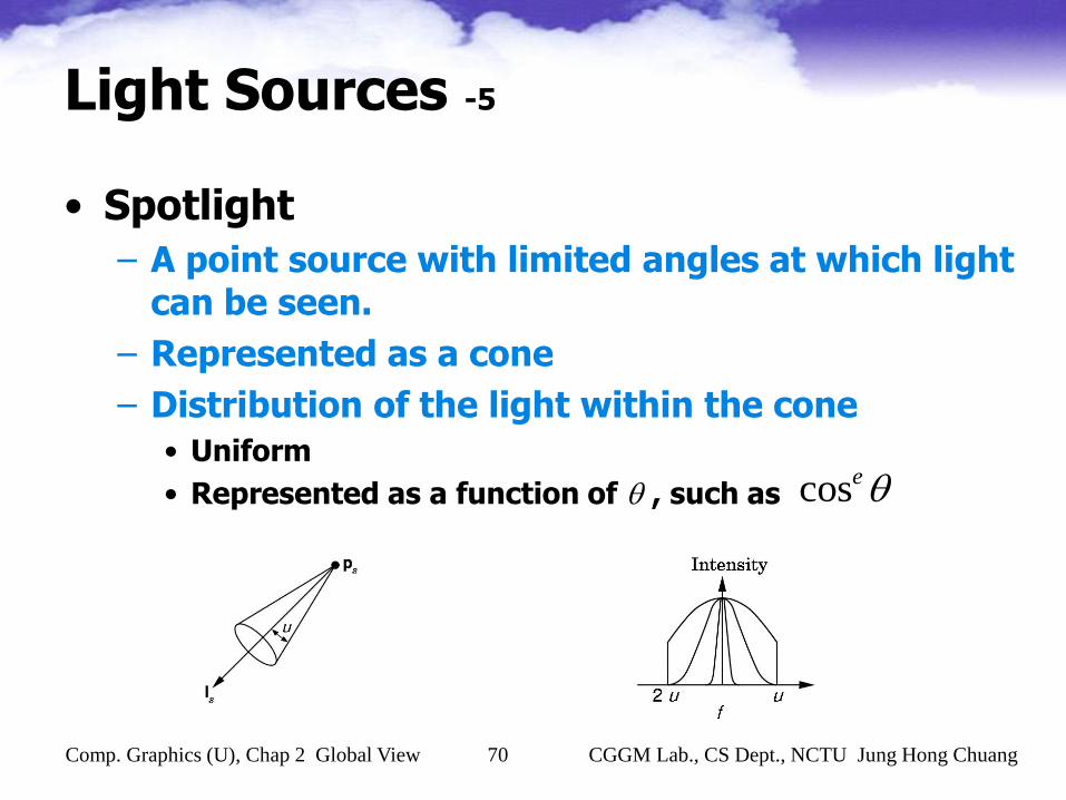
Light Sources -5
• Spotlight
– A point source with limited angles at which light can be seen.
– Represented as a cone
– Distribution of the light within the cone
• Uniform
• Represented as a function of , such as ecos

Comp. Graphics (U), Chap 2 Global View 71 CGGM Lab., CS Dept., NCTU Jung Hong Chuang
Light Sources -6
• Distant light sources
– The light source is far from the surface.
– The source becomes point sources
– Illuminate objects with parallel rays of light
– In calculation, the location of the source is replaced by the direction of the parallel rays

Comp. Graphics (U), Chap 2 Global View 72 CGGM Lab., CS Dept., NCTU Jung Hong Chuang
Light and matter -1
• Light and surface
– We see the color of the light reflected from the surface toward our eyes
– Human’s perception vs. computer image

Comp. Graphics (U), Chap 2 Global View 73 CGGM Lab., CS Dept., NCTU Jung Hong Chuang
Light and matter -2
• Light-material interaction
– When light strikes a surface, some of it is absorbed, some of it is reflected, and some of it is transmitted through the material
– Specular surfaces, diffuse surfaces, translucent surfaces

Comp. Graphics (U), Chap 2 Global View 74 CGGM Lab., CS Dept., NCTU Jung Hong Chuang
Light and matter -3
Light incidents at a point will be reflected, absorbed, scattered, and transmitted

Comp. Graphics (U), Chap 2 Global View 75 CGGM Lab., CS Dept., NCTU Jung Hong Chuang
Phong Reflection Model -1
• A simple model that compromises between acceptable results and processing cost.
– Computes light intensity at a surface point, assuming point light source.
– Considers only local lighting reflected and regards global lighting as an ambient term.
• Other reflection models
– Cook and Torrance model
– Warn’s method for modeling illumination source
– BRDF/BSSRDF model

Comp. Graphics (U), Chap 2 Global View 76 CGGM Lab., CS Dept., NCTU Jung Hong Chuang
Phong Reflection Model -2
XXXxX
Approximates local lighting Approximates global lighting

Comp. Graphics (U), Chap 2 Global View 77 CGGM Lab., CS Dept., NCTU Jung Hong Chuang
Phong Reflection Model -3
• An efficient computation of light-material interactions.
• Consists of three terms
– Ambient term
– Diffuse term
– Specular term
))()( ] [(1
] [2
vrLknILkcdbda
LkI sdaa

Comp. Graphics (U), Chap 2 Global View 78 CGGM Lab., CS Dept., NCTU Jung Hong Chuang
Diffuse Reflection
• A perfect diffuse scatters light equally in all directions, independent on the viewer's position
– appears equally bright from all views
• Responsible for the color of the object
– Example: A green object absorbs white light and reflects the green component of the light
• It is characterized by rough surfaces
– Light rays with slightly different angles
are reflected at markedly different angles.Perfectly diffuse surfaces are so rough that there is no preferred angle of reflection.

Comp. Graphics (U), Chap 2 Global View 79 CGGM Lab., CS Dept., NCTU Jung Hong Chuang
Diffuse Term -1
• Intensity of the diffuse reflected light
Id = Kd Ii cos
– Ii : the intensity of the light source
– : angle between the surface normal n and the vector l
from the surface point to the point light source
– Kd : wavelength-dependent diffuse reflectivity, 0 < Kd < 1
• Note that cos = l ·n
where l is a unit vector pointing
from the surface point to the light source

Comp. Graphics (U), Chap 2 Global View 80 CGGM Lab., CS Dept., NCTU Jung Hong Chuang
Diffuse Term -2

Comp. Graphics (U), Chap 2 Global View 81 CGGM Lab., CS Dept., NCTU Jung Hong Chuang
Specular Reflection -1
• For a perfect reflector, reflected light is seen only in the direction of R
– In practice, specular reflection is not perfect and reflected light can be seen for viewing directions close to the direction of R (and produce highlight)
Comp. Graphics (U), Chap 2 Global View 82 CGGM Lab., CS Dept., NCTU Jung Hong Chuang
Specular Reflection -2
• A highlight is a surface area from which the viewer can see the specular reflection
• Reflection range ( or highlight area) depends on the surface roughness
• The color of the specular reflection is the color of the light source
– For example
• A green surface illuminated by white light has color green from diffuse reflection and color white from specular reflection.

Comp. Graphics (U), Chap 2 Global View 83 CGGM Lab., CS Dept., NCTU Jung Hong Chuang
Specular Term -1
– ns simulates the surface roughness:
• perfect specular H-A : 0 ns : ∞
• very glossy surface H-A : smaller ns : large
• less glossy surface H-A : large ns : smaller
– Ks is the specular reflection coefficient which depends on surface property and .
• Transparent material
– Ks() is 1 when = 90 and decrease when decreases.
• Opaque materials
– Ks() is nearly constant for any
ssn
si
n
sis VRKIKII cos

Comp. Graphics (U), Chap 2 Global View 84 CGGM Lab., CS Dept., NCTU Jung Hong Chuang
Specular Term -2

Comp. Graphics (U), Chap 2 Global View 85 CGGM Lab., CS Dept., NCTU Jung Hong Chuang
Ambient Term
• For surfaces that are visible from the view point but invisible from the point light source, should we render black?
– No, made visible by ambient light since they are illuminated by other objects
– Ambient term is the result of multiple reflection from walls and objects, and is incident on a surface from all directions.

Comp. Graphics (U), Chap 2 Global View 86 CGGM Lab., CS Dept., NCTU Jung Hong Chuang
Ambient Term
• It can be approximated by a constant
I = Ia ka
where Ia is a user-specified constant that approximates the global lighting effect and ka is the ambient reflection coefficient

Comp. Graphics (U), Chap 2 Global View 87 CGGM Lab., CS Dept., NCTU Jung Hong Chuang
Phong Model - 1
• Control the color of the objects by appropriate setting of the diffuse reflection coefficients.
• Color of light sources are controlled by the specular reflection coefficients.

Comp. Graphics (U), Chap 2 Global View 88 CGGM Lab., CS Dept., NCTU Jung Hong Chuang
Phong Model - 2
Comp. Graphics (U), Chap 2 Global View 89 CGGM Lab., CS Dept., NCTU Jung Hong Chuang
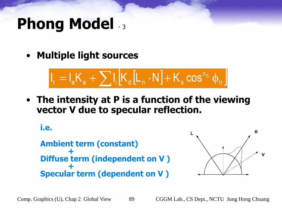
Phong Model - 3
• Multiple light sources
• The intensity at P is a function of the viewing vector V due to specular reflection.
i.e.
Ambient term (constant)+
Diffuse term (independent on V )+
Specular term (dependent on V )

Comp. Graphics (U), Chap 2 Global View 90 CGGM Lab., CS Dept., NCTU Jung Hong Chuang
Note onComputing vectors• Normal vectors
– Triangle normal
– Vertex normal
– Plane• Plane equation
• Three non-coplanar points
– Implicit surfaces• F(x, y, z)=0
– Parametric surfaces• P(u, v)
• Angle of reflection

Comp. Graphics (U), Chap 2 Global View 91 CGGM Lab., CS Dept., NCTU Jung Hong Chuang
Shading
• Apply a "point" reflection model over the entire surface of an object is impossible
• Polygon shading methods– Constant shading
– Gouraud shading• Pixel’s intensity is obtained by bilinear interpolation of
vertex’s intensities
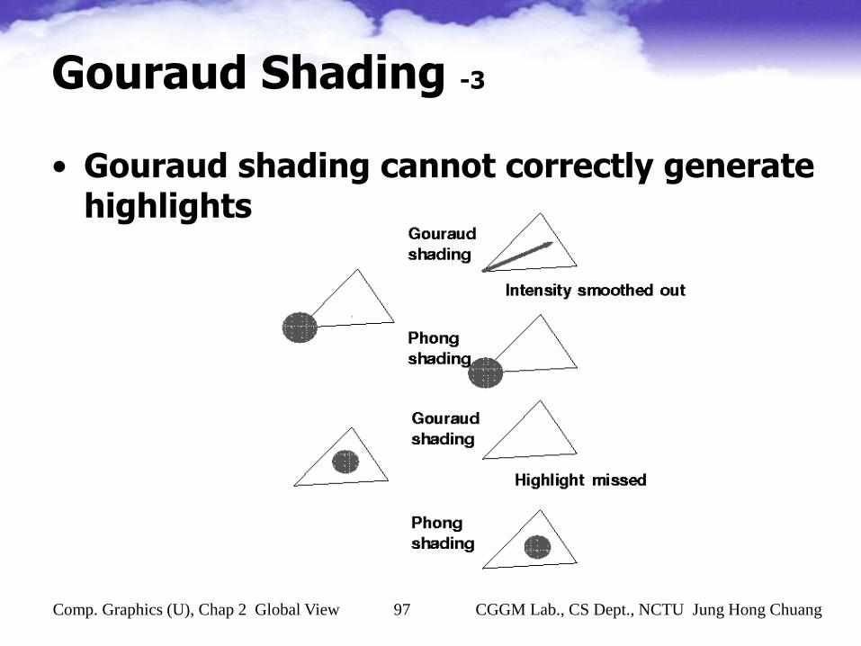
• Produces incorrect highlights on a polygon
– Phong shading• Pixel’s normal is obtained by bilinear interpolation of
vertex’s normals
• Can give more accurate specular effects

Comp. Graphics (U), Chap 2 Global View 92 CGGM Lab., CS Dept., NCTU Jung Hong Chuang
Shading
Normal interpolation

Comp. Graphics (U), Chap 2 Global View 93 CGGM Lab., CS Dept., NCTU Jung Hong ChuangIntro. to VR, Chap.4 Visualizing the VE 93 CGGM Lab.,CSIE Dept.,NCTU Jung Hong Chuang

Comp. Graphics (U), Chap 2 Global View 94 CGGM Lab., CS Dept., NCTU Jung Hong ChuangIntro. to VR, Chap.4 Visualizing the VE 94 CGGM Lab.,CSIE Dept.,NCTU Jung Hong Chuang

Comp. Graphics (U), Chap 2 Global View 95 CGGM Lab., CS Dept., NCTU Jung Hong Chuang
Gouraud Shading -1
• Compute (in world coord. system) the intensity at each vertex of the polygon by Phong model
– N is in general the surface normal at the vertex, can be approximated by the average of the normals of the adjacent polygons.
– When polygons are clipped, the normals at clipped vertices are interpolated in world coord. or view coord.

Comp. Graphics (U), Chap 2 Global View 96 CGGM Lab., CS Dept., NCTU Jung Hong Chuang
Gouraud Shading -2
• Interpolate the intensities over the polygon
• Incremental calculation
– x: incremental change along a scan line
– IS: change in intensity
Comp. Graphics (U), Chap 2 Global View 97 CGGM Lab., CS Dept., NCTU Jung Hong Chuang
Gouraud Shading -3
• Gouraud shading cannot correctly generate highlights
Comp. Graphics (U), Chap 2 Global View 98 CGGM Lab., CS Dept., NCTU Jung Hong Chuang
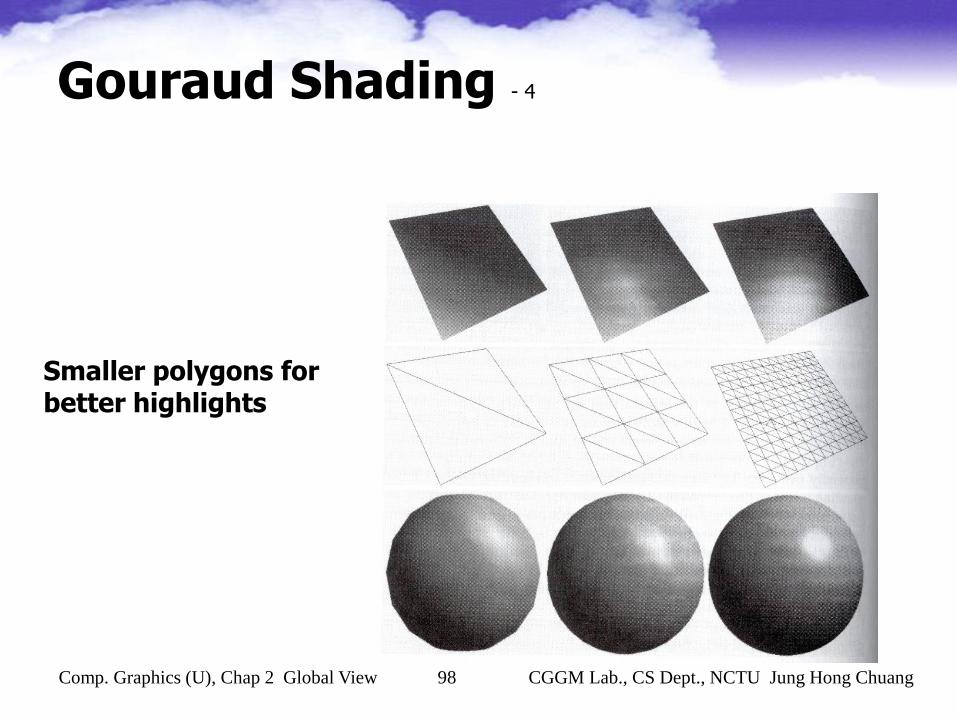
Gouraud Shading - 4
Smaller polygons for better highlights

Comp. Graphics (U), Chap 2 Global View 99 CGGM Lab., CS Dept., NCTU Jung Hong Chuang
Phong Shading -1
• Interpolate normals instead of intensities
– Compute the vertex normals
– Interpolate the normal for interior point (in screen coord. system)
– Compute the intensity at interior point (in world coord. System, or view coord. system)
• Phong shading is computationally more expensive than Gouraud shading

Comp. Graphics (U), Chap 2 Global View 100 CGGM Lab., CS Dept., NCTU Jung Hong Chuang
Phong Shading - 2
• Incremental calculation– x: incremental change along a scan line– IS: change in intensity
SNSNS
ab
ab
S
NNN
NNxx
xN
1,,

Comp. Graphics (U), Chap 2 Global View 101 CGGM Lab., CS Dept., NCTU Jung Hong Chuang
Phong Shading - 3
Ks: increases from left, Ns: increases from top; Ka and Kd: constant

Comp. Graphics (U), Chap 2 Global View 102 CGGM Lab., CS Dept., NCTU Jung Hong Chuang
Rendering Pipeline
• Set up a polygonal mesh for the scene.
• Culling back-facing polygons.
(in WC, or view coord, or screen coord.)
• Apply viewing transformation and projection.
• Clip polygons against view volume.
(in 3D screen space or homogeneous space)
• Scan convert polygons.
• Shade pixels by incremental shading methods.
• Apply hidden surface removal: Z-buffer.

Comp. Graphics (U), Chap 2 Global View 103 CGGM Lab., CS Dept., NCTU Jung Hong Chuang
Z-Buffer HSR - 1
• A duplicate memory in the size of frame buffer holds the of depths for each pixel in the frame buffer.
– A current point (i, j ) holds the smallest z-value so far encountered. During the processing of a polygon, we either write the intensity of (i, j ) into the frame buffer or not, depending on whether the depth z < Z-Buffer(i, j )

Comp. Graphics (U), Chap 2 Global View 104 CGGM Lab., CS Dept., NCTU Jung Hong Chuang
Z-Buffer HSR - 2

Comp. Graphics (U), Chap 2 Global View 105 CGGM Lab., CS Dept., NCTU Jung Hong Chuang
Z-Buffer HSR - 3

Comp. Graphics (U), Chap 2 Global View 106 CGGM Lab., CS Dept., NCTU Jung Hong Chuang
Z-Buffer HSR - 4

Comp. Graphics (U), Chap 2 Global View 107 CGGM Lab., CS Dept., NCTU Jung Hong Chuang
Z-Buffer HSR - 5

Comp. Graphics (U), Chap 2 Global View 108 CGGM Lab., CS Dept., NCTU Jung Hong Chuang
Z-buffer HSR - 6
• Advantage of Z-buffer method
– Easy to implement and usually hardware supported.
– No upward limit on the scene complexity.
• Disadvantages
– Space consuming is very high.
• 23-32 bits per pixel is usually deemed sufficient.
– The scene has to be scaled to this fixed range of z so accuracy within the scene is maximized.

Comp. Graphics (U), Chap 2 Global View 109 CGGM Lab., CS Dept., NCTU Jung Hong Chuang
Z-buffer HSR - 7
/* polygon by polygon basis, with polygon inany convenient order */
for all (x,y) do Z-buffer(x,y) := maximum-depth;for each polygon do
for y = ymin to ymax do/* scan convert one scan-line at a time */
begincalculate x, z, and l for left/right end points:
Xleft, Xright, Zleft, Zright, lleft, lrightfor x = xleft to xright do
linearly interpolate z & lif z < Z-buffer(x,y) then
Z-buffer(x, y) := z ;Frame-buffer(x, y) := l ;
end

Comp. Graphics (U), Chap 2 Global View 110 CGGM Lab., CS Dept., NCTU Jung Hong Chuang
Rendering PipelineDetail Steps

Global Illumination, texture Mapping, multi-pass renderingPipeline supported:• Texture mapping techniques
– Multi-texturing, bump map, displacement map, light map, normal map, environment map, shadow map…
• Multi-pass rendering• Shadow Computing
– Improve depth cues– View-independent– Hard shadow vs. soft shadow
Comp. Graphics (U), Chap 2 Global View 111 CGGM Lab., CS Dept., NCTU Jung Hong Chuang

Comp. Graphics (U), Chap 2 Global View 112 CGGM Lab., CS Dept., NCTU Jung Hong Chuang
Global Illumination, texture Mapping, multi-pass renderingNot supported by fixed pipeline• Global illumination
– Ray tracing, Monte Carlo ray tracing, Photon maps• Ray tracing: Good for specular scenes• Monte Carlo ray tracing, Photon maps: good
for many types of surface• View-dependent, naturally for dynamic scenes,
can be GPU accelerated– Radiosity
• Good for diffuse scenes• View-independent, Practically useful for static
navigation

Comp. Graphics (U), Chap 2 Global View 113 CGGM Lab., CS Dept., NCTU Jung Hong Chuang
Examples for Different Methods
Gouraud shading Phong shading
Environment mapping & shadowing
Texture mapping
Ray tracing Radiosity

Comp. Graphics (U), Chap 2 Global View 114 CGGM Lab., CS Dept., NCTU Jung Hong Chuang
Radiance Example

Comp. Graphics (U), Chap 2 Global View 115 CGGM Lab., CS Dept., NCTU Jung Hong Chuang

Comp. Graphics (U), Chap 2 Global View 116 CGGM Lab., CS Dept., NCTU Jung Hong Chuang

Comp. Graphics (U), Chap 2 Global View 117 CGGM Lab., CS Dept., NCTU Jung Hong Chuang

Comp. Graphics (U), Chap 2 Global View 118 CGGM Lab., CS Dept., NCTU Jung Hong Chuang
Texture mapping
A plane
A cylinder
A sphere

Comp. Graphics (U), Chap 2 Global View 119 CGGM Lab., CS Dept., NCTU Jung Hong Chuang
Multitexturing
Light mapTexture map

Comp. Graphics (U), Chap 2 Global View 120 CGGM Lab., CS Dept., NCTU Jung Hong Chuang
3D Texture Mapping

Comp. Graphics (U), Chap 2 Global View 121 CGGM Lab., CS Dept., NCTU Jung Hong Chuang
Bump Mapping

Comp. Graphics (U), Chap 2 Global View 122 CGGM Lab., CS Dept., NCTU Jung Hong Chuang
Bump Mapping

Comp. Graphics (U), Chap 2 Global View 123 CGGM Lab., CS Dept., NCTU Jung Hong Chuang
Bump mapping
Bump map + shadowing
md2shader demo!!
Comp. Graphics (U), Chap 2 Global View 124 CGGM Lab., CS Dept., NCTU Jung Hong Chuang
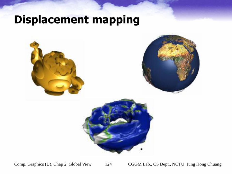
Displacement mapping

Comp. Graphics (U), Chap 2 Global View 125 CGGM Lab., CS Dept., NCTU Jung Hong Chuang
Normal map
OriginalM5
M5+NMNormal maps

Comp. Graphics (U), Chap 2 Global View 126 CGGM Lab., CS Dept., NCTU Jung Hong Chuang
Multi-pass rendering

Comp. Graphics (U), Chap 2 Global View 127 CGGM Lab., CS Dept., NCTU Jung Hong Chuang
Multi-pass renderingGloss mapping
http://www.opengl.org/developers/code/sig99/shading99/course_slides/ShadingComputations/sld026.htm

Comp. Graphics (U), Chap 2 Global View 128 CGGM Lab., CS Dept., NCTU Jung Hong Chuang
Multi-pass renderingLight mapping
WithoutLight map
[From Channa’s article]

Comp. Graphics (U), Chap 2 Global View 129 CGGM Lab., CS Dept., NCTU Jung Hong Chuang
Multi-pass renderingLight mapping
WithLight map
The white rhombus type object (on the right hand side) represents a point light source.
[From Channa’s article]
Comp. Graphics (U), Chap 2 Global View 130 CGGM Lab., CS Dept., NCTU Jung Hong Chuang
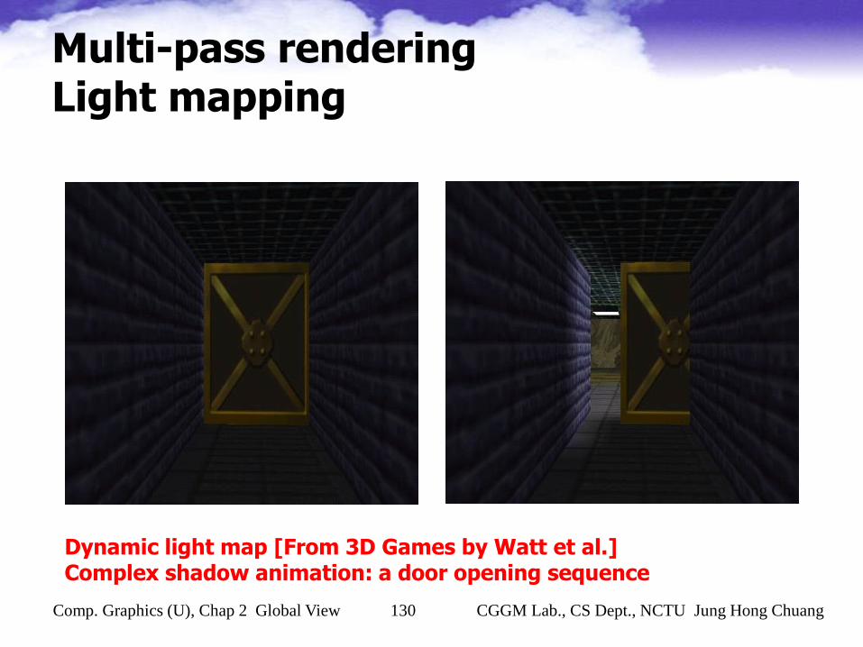
Multi-pass rendering Light mapping
Dynamic light map [From 3D Games by Watt et al.]Complex shadow animation: a door opening sequence

Comp. Graphics (U), Chap 2 Global View 131 CGGM Lab., CS Dept., NCTU Jung Hong Chuang
Multi-pass rendering Light mapping
Dynamic light mapComplex shadow animation: a door opening sequence

Comp. Graphics (U), Chap 2 Global View 132 CGGM Lab., CS Dept., NCTU Jung Hong Chuang
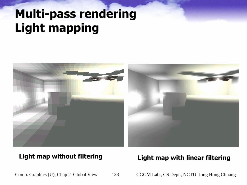
Multi-pass rendering Light mapping
Texture map without filtering[From 3D Games, by Watt et al.]
Texture map with mipmapping
Another example
Comp. Graphics (U), Chap 2 Global View 133 CGGM Lab., CS Dept., NCTU Jung Hong Chuang
Multi-pass rendering Light mapping
Light map without filtering Light map with linear filtering

Comp. Graphics (U), Chap 2 Global View 134 CGGM Lab., CS Dept., NCTU Jung Hong Chuang
Multi-pass rendering Light mapping
With mipmapped texture and filtered light map
Fog map with linear filtering

Comp. Graphics (U), Chap 2 Global View 135 CGGM Lab., CS Dept., NCTU Jung Hong Chuang
Multi-pass rendering Light mapping
With mipmappedtexture and linearfiltered light,and fog map.

Comp. Graphics (U), Chap 2 Global View 136 CGGM Lab., CS Dept., NCTU Jung Hong Chuang
Multi-pass rendering Light mapping
Without Light map
Another example

Comp. Graphics (U), Chap 2 Global View 137 CGGM Lab., CS Dept., NCTU Jung Hong Chuang
Multi-pass rendering Light mapping
With lightmap
Comp. Graphics (U), Chap 2 Global View 138 CGGM Lab., CS Dept., NCTU Jung Hong Chuang
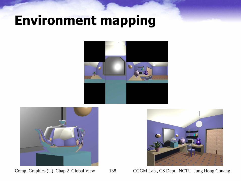
Environment mapping
Environment map
on a box
Result A room scene

Comp. Graphics (U), Chap 2 Global View 139 CGGM Lab., CS Dept., NCTU Jung Hong Chuang
Environment mapping A Comparison to Ray Tracing
Ray tracing
Environment
mapping

Comp. Graphics (U), Chap 2 Global View 140 CGGM Lab., CS Dept., NCTU Jung Hong Chuang
Multi-pass shadowing Properties -2
Sphere on a plane of infinite extent
The sphere rests on the plane
The sphere is slightly above the plane
No shadow
Shadow provides information about the relative positions of objects[From Real-Time Soft Shadow]

Comp. Graphics (U), Chap 2 Global View 141 CGGM Lab., CS Dept., NCTU Jung Hong Chuang
Multi-pass shadowing Properties -3
Sphere on a plane of infinite extent
The sphere rests on the plane
The sphere is slightly above the plane
No shadow
Shadow provides information about the geometry of the occluder[From Real-Time Soft Shadow]

Comp. Graphics (U), Chap 2 Global View 142 CGGM Lab., CS Dept., NCTU Jung Hong Chuang
Multi-pass shadowing Properties -4
Sphere on a plane of infinite extent
The sphere rests on the plane
The sphere is slightly above the plane
No shadow
Shadow provides information about the geometry of the receiver[From Real-Time Soft Shadow]

Comp. Graphics (U), Chap 2 Global View 143 CGGM Lab., CS Dept., NCTU Jung Hong Chuang
Hard shadows
Three colored lights.
Diffuse/specular bump
mapped animated
characters with
shadows. 34 fps on
GeForce4 Ti 4600;
80+ fps for one light.
[Everitt & Kilgard]

Comp. Graphics (U), Chap 2 Global View 144 CGGM Lab., CS Dept., NCTU Jung Hong Chuang
Soft shadows
Cluster of 12 dim
lights approximating
an area light source.
Generates a soft
shadow effect; careful
about banding. 8 fps on
GeForce4 Ti 4600.
The cluster of
point lights.
[Everitt & Kilgard]