Major Contributors:Patricia Grossi

Howard KunreutherDon Windeler

This chapter provides an overview of the history of catastrophemodels and their role in risk assessment and management of natural disasters.It examines the insurability of catastrophe risk and illustrates how the outputfrom catastrophe models aids insurers in meeting their goals for riskmanagement. Throughout the chapter, there is an emphasis on understandingcatastrophe modeling for earthquake and hurricane hazards and how it is usedto manage natural hazard risk. In the final section, a framework for integratingrisk assessment with risk management via catastrophe modeling is presented.

2.1 History of Catastrophe ModelsCatastrophe modeling is not rooted in one field or discipline. The

science of assessing and managing catastrophe risk originates in the fields ofproperty insurance and the science of natural hazards. Insurers may well arguethat catastrophe modeling’s history lies in the earliest days of propertyinsurance coverage for fire and lightning. In the 1800’s, residential insurersmanaged their risk by mapping the structures that they covered. Not havingaccess to Geographic Information Systems (GIS) software, they used tacks ona wall-hung map to indicate their concentration of exposure. This crudetechnique served insurers well and limited their risk. Widespread usage ofmapping ended in the 1960’s when it became too cumbersome and time-consuming to execute (Kozlowski and Mathewson, 1995).

On the other hand, a seismologist or meteorologist may well arguethat the origin of catastrophe modeling lies in the modern science ofunderstanding the nature and impact of natural hazards. In particular, thecommon practice of measuring an earthquake’s magnitude and a hurricane’sintensity is one of the key ingredients in catastrophe modeling. A standard set

Chapter 2 – An Introduction to Catastrophe Modelsand Insurance

24

of metrics for a given hazard must be established so that risks can be assessedand managed. This measurement began in the 1800’s, when the first modernseismograph (measuring earthquake ground motion) was invented andmodern versions of the anemometer (measuring wind speed) gainedwidespread usage.

In the first part of the twentieth century, scientific measures of naturalhazards advanced rapidly. By the 1970’s, studies theorizing on the source andfrequency of events were published. Significant analyses include the U.S.Water Resources Council publication on flood hazard (USWRC, 1967), theAlgermissen study on earthquake risk (Algermissen, 1969) and NationalOceanic and Atmospheric Administration (NOAA) hurricane forecasts(Neumann, 1972). These developments led U.S. researchers to compile hazardand loss studies, estimating the impact of earthquakes, hurricanes, floods, andother natural disasters. Notable compilations include Brinkmann’s summaryof hurricane hazards in the United States (1975) and Steinbrugge’s anthologyof losses from earthquakes, volcanoes, and tsunamis (1982).

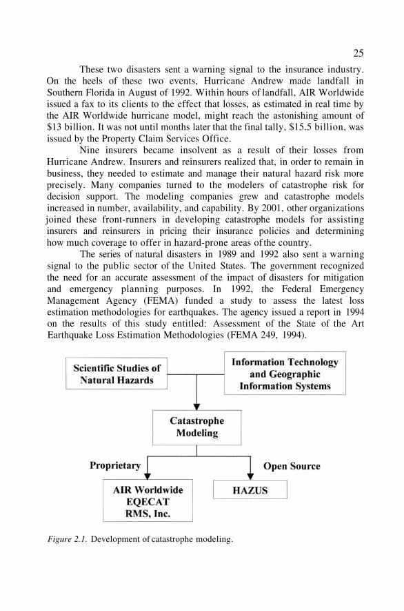
These two separate developments – mapping risk and measuringhazard – came together in a definitive way in the late 1980’s and early 1990’s,through catastrophe modeling as shown in Figure 2.1. Computer-basedmodels for measuring catastrophe loss potential were developed by linkingscientific studies of natural hazards’ measures and historical occurrences withadvances in information technology and geographic information systems(GIS). The models provided estimates of catastrophe losses by overlaying theproperties at risk with the potential natural hazard(s) sources in the geographicarea. With the ability to store and manage vast amounts of spatially referencedinformation, GIS became an ideal environment for conducting easier andmore cost-effective hazard and loss studies.

Around the same time, several new modeling firms developedcomputer software for analyzing the implications of natural hazard risk. Threemajor firms emerged: AIR Worldwide was founded in 1987 in Boston; RiskManagement Solutions (RMS) was formed in 1988 at Stanford University;and EQECAT began in San Francisco in 1994 as a subsidiary of EQEInternational. In 2001, EQE International became a part of ABS Consulting.

When introduced, the use of catastrophe models was not widespread.In 1989, two large-scale disasters occurred that instigated a flurry of activityin the advancement and use of these models. On September 21, 1989,Hurricane Hugo hit the coast of South Carolina, devastating the towns ofCharleston and Myrtle Beach. Insured loss estimates totaled $4 billion beforethe storm moved through North Carolina the next day (Insurance InformationInstitute, 2000). Less than a month later, on October 17, 1989, the LomaPrieta Earthquake occurred at the southern end of the San Franciscopeninsula. Property damage to the surrounding Bay Area was estimated at $6billion (Stover and Coffman, 1993).

25

These two disasters sent a warning signal to the insurance industry.On the heels of these two events, Hurricane Andrew made landfall inSouthern Florida in August of 1992. Within hours of landfall, AIR Worldwideissued a fax to its clients to the effect that losses, as estimated in real time bythe AIR Worldwide hurricane model, might reach the astonishing amount of$13 billion. It was not until months later that the final tally, $15.5 billion, wasissued by the Property Claim Services Office.

Nine insurers became insolvent as a result of their losses fromHurricane Andrew. Insurers and reinsurers realized that, in order to remain inbusiness, they needed to estimate and manage their natural hazard risk moreprecisely. Many companies turned to the modelers of catastrophe risk fordecision support. The modeling companies grew and catastrophe modelsincreased in number, availability, and capability. By 2001, other organizationsjoined these front-runners in developing catastrophe models for assistinginsurers and reinsurers in pricing their insurance policies and determininghow much coverage to offer in hazard-prone areas of the country.

The series of natural disasters in 1989 and 1992 also sent a warningsignal to the public sector of the United States. The government recognizedthe need for an accurate assessment of the impact of disasters for mitigationand emergency planning purposes. In 1992, the Federal EmergencyManagement Agency (FEMA) funded a study to assess the latest lossestimation methodologies for earthquakes. The agency issued a report in 1994on the results of this study entitled: Assessment of the State of the ArtEarthquake Loss Estimation Methodologies (FEMA 249, 1994).

Figure 2.1. Development of catastrophe modeling.

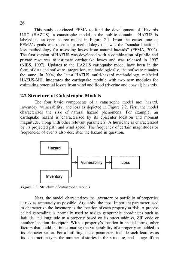
26This study convinced FEMA to fund the development of “Hazards

U.S.” (HAZUS), a catastrophe model in the public domain. HAZUS islabeled as an open source model in Figure 2.1. From the outset, one ofFEMA’s goals was to create a methodology that was the “standard nationalloss methodology for assessing losses from natural hazards” (FEMA, 2002).The first version of HAZUS was developed with a combination of public andprivate resources to estimate earthquake losses and was released in 1997(NIBS, 1997). Updates to the HAZUS earthquake model have been in theform of data and software integration; methodologically, the software remainsthe same. In 2004, the latest HAZUS multi-hazard methodology, relabeledHAZUS-MH, integrates the earthquake module with two new modules forestimating potential losses from wind and flood (riverine and coastal) hazards.

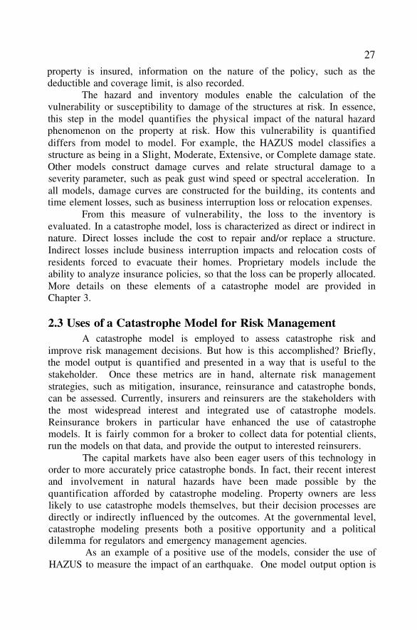
2.2 Structure of Catastrophe ModelsThe four basic components of a catastrophe model are: hazard,

inventory, vulnerability, and loss as depicted in Figure 2.2. First, the modelcharacterizes the risk of natural hazard phenomena. For example, anearthquake hazard is characterized by its epicenter location and momentmagnitude, along with other relevant parameters. A hurricane is characterizedby its projected path and wind speed. The frequency of certain magnitudes orfrequencies of events also describes the hazard in question.

Figure 2.2. Structure of catastrophe models.

Next, the model characterizes the inventory or portfolio of propertiesat risk as accurately as possible. Arguably, the most important parameter usedto characterize the inventory is the location of each property at risk. A processcalled geocoding is normally used to assign geographic coordinates such aslatitude and longitude to a property based on its street address, ZIP code oranother location descriptor. With a property’s location in spatial terms, otherfactors that could aid in estimating the vulnerability of a property are added toits characterization. For a building, these parameters include such features asits construction type, the number of stories in the structure, and its age. If the

27

property is insured, information on the nature of the policy, such as thedeductible and coverage limit, is also recorded.

The hazard and inventory modules enable the calculation of thevulnerability or susceptibility to damage of the structures at risk. In essence,this step in the model quantifies the physical impact of the natural hazardphenomenon on the property at risk. How this vulnerability is quantifieddiffers from model to model. For example, the HAZUS model classifies astructure as being in a Slight, Moderate, Extensive, or Complete damage state.Other models construct damage curves and relate structural damage to aseverity parameter, such as peak gust wind speed or spectral acceleration. Inall models, damage curves are constructed for the building, its contents andtime element losses, such as business interruption loss or relocation expenses.

From this measure of vulnerability, the loss to the inventory isevaluated. In a catastrophe model, loss is characterized as direct or indirect innature. Direct losses include the cost to repair and/or replace a structure.Indirect losses include business interruption impacts and relocation costs ofresidents forced to evacuate their homes. Proprietary models include theability to analyze insurance policies, so that the loss can be properly allocated.More details on these elements of a catastrophe model are provided inChapter 3.

2.3 Uses of a Catastrophe Model for Risk ManagementA catastrophe model is employed to assess catastrophe risk and

improve risk management decisions. But how is this accomplished? Briefly,the model output is quantified and presented in a way that is useful to thestakeholder. Once these metrics are in hand, alternate risk managementstrategies, such as mitigation, insurance, reinsurance and catastrophe bonds,can be assessed. Currently, insurers and reinsurers are the stakeholders withthe most widespread interest and integrated use of catastrophe models.Reinsurance brokers in particular have enhanced the use of catastrophemodels. It is fairly common for a broker to collect data for potential clients,run the models on that data, and provide the output to interested reinsurers.

The capital markets have also been eager users of this technology inorder to more accurately price catastrophe bonds. In fact, their recent interestand involvement in natural hazards have been made possible by thequantification afforded by catastrophe modeling. Property owners are lesslikely to use catastrophe models themselves, but their decision processes aredirectly or indirectly influenced by the outcomes. At the governmental level,catastrophe modeling presents both a positive opportunity and a politicaldilemma for regulators and emergency management agencies.

As an example of a positive use of the models, consider the use ofHAZUS to measure the impact of an earthquake. One model output option is

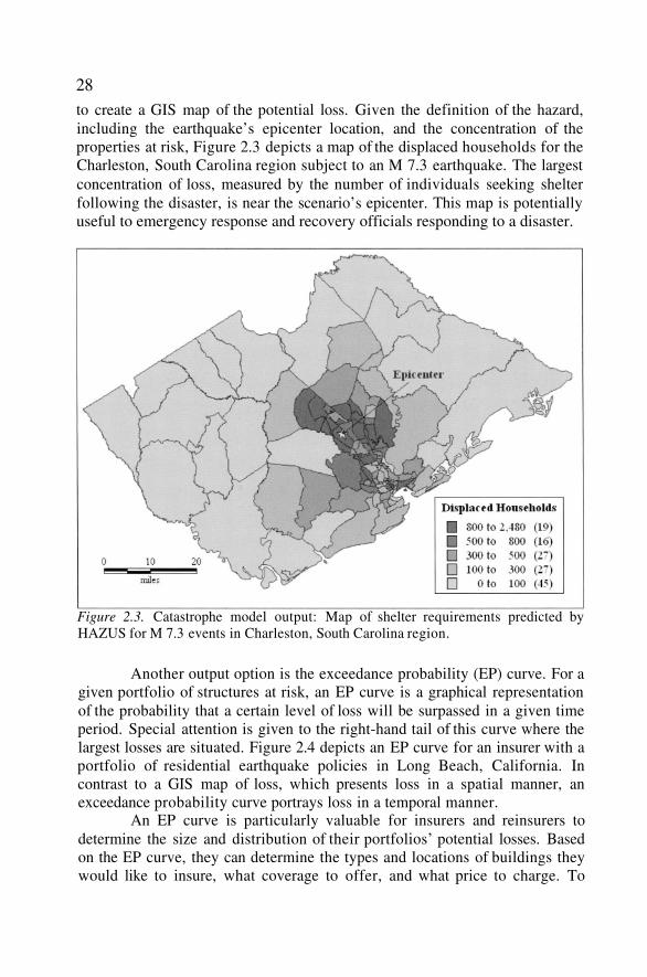
28to create a GIS map of the potential loss. Given the definition of the hazard,including the earthquake’s epicenter location, and the concentration of theproperties at risk, Figure 2.3 depicts a map of the displaced households for theCharleston, South Carolina region subject to an M 7.3 earthquake. The largestconcentration of loss, measured by the number of individuals seeking shelterfollowing the disaster, is near the scenario’s epicenter. This map is potentiallyuseful to emergency response and recovery officials responding to a disaster.

Figure 2.3. Catastrophe model output: Map of shelter requirements predicted byHAZUS for M 7.3 events in Charleston, South Carolina region.

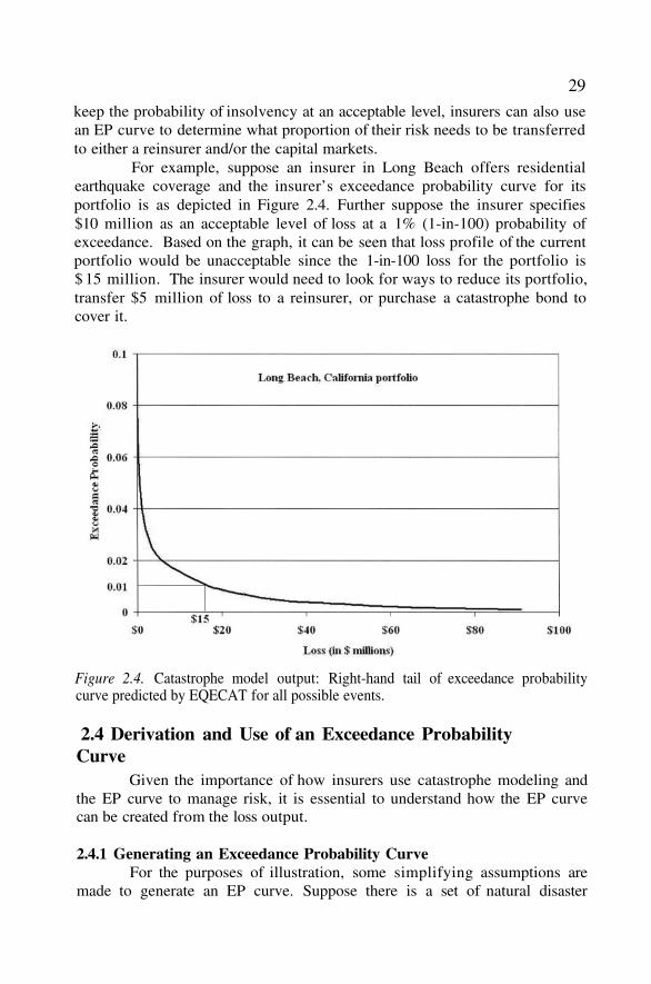
Another output option is the exceedance probability (EP) curve. For agiven portfolio of structures at risk, an EP curve is a graphical representationof the probability that a certain level of loss will be surpassed in a given timeperiod. Special attention is given to the right-hand tail of this curve where thelargest losses are situated. Figure 2.4 depicts an EP curve for an insurer with aportfolio of residential earthquake policies in Long Beach, California. Incontrast to a GIS map of loss, which presents loss in a spatial manner, anexceedance probability curve portrays loss in a temporal manner.

An EP curve is particularly valuable for insurers and reinsurers todetermine the size and distribution of their portfolios’ potential losses. Basedon the EP curve, they can determine the types and locations of buildings theywould like to insure, what coverage to offer, and what price to charge. To

29

keep the probability of insolvency at an acceptable level, insurers can also usean EP curve to determine what proportion of their risk needs to be transferredto either a reinsurer and/or the capital markets.

For example, suppose an insurer in Long Beach offers residentialearthquake coverage and the insurer’s exceedance probability curve for itsportfolio is as depicted in Figure 2.4. Further suppose the insurer specifies$10 million as an acceptable level of loss at a 1% (1-in-100) probability ofexceedance. Based on the graph, it can be seen that loss profile of the currentportfolio would be unacceptable since the 1-in-100 loss for the portfolio is$ 15 million. The insurer would need to look for ways to reduce its portfolio,transfer $5 million of loss to a reinsurer, or purchase a catastrophe bond tocover it.

Figure 2.4. Catastrophe model output: Right-hand tail of exceedance probabilitycurve predicted by EQECAT for all possible events.

2.4 Derivation and Use of an Exceedance ProbabilityCurve

Given the importance of how insurers use catastrophe modeling andthe EP curve to manage risk, it is essential to understand how the EP curvecan be created from the loss output.

2.4.1 Generating an Exceedance Probability CurveFor the purposes of illustration, some simplifying assumptions are

made to generate an EP curve. Suppose there is a set of natural disaster

30

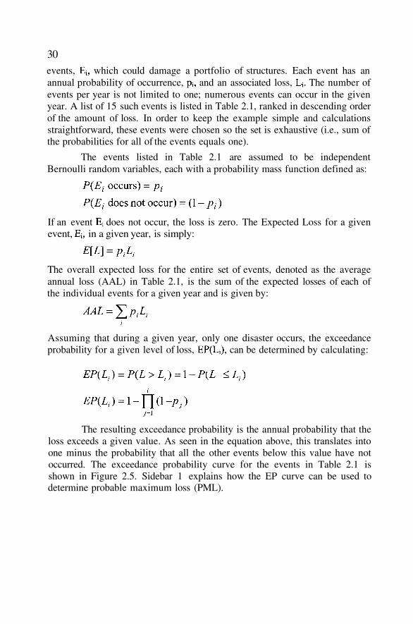
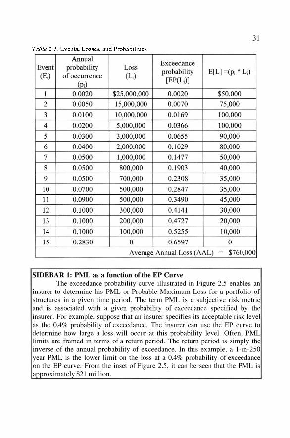
events, which could damage a portfolio of structures. Each event has anannual probability of occurrence, and an associated loss, The number ofevents per year is not limited to one; numerous events can occur in the givenyear. A list of 15 such events is listed in Table 2.1, ranked in descending orderof the amount of loss. In order to keep the example simple and calculationsstraightforward, these events were chosen so the set is exhaustive (i.e., sum ofthe probabilities for all of the events equals one).

The events listed in Table 2.1 are assumed to be independentBernoulli random variables, each with a probability mass function defined as:

If an event does not occur, the loss is zero. The Expected Loss for a givenevent, in a given year, is simply:

The overall expected loss for the entire set of events, denoted as the averageannual loss (AAL) in Table 2.1, is the sum of the expected losses of each ofthe individual events for a given year and is given by:

Assuming that during a given year, only one disaster occurs, the exceedanceprobability for a given level of loss, can be determined by calculating:

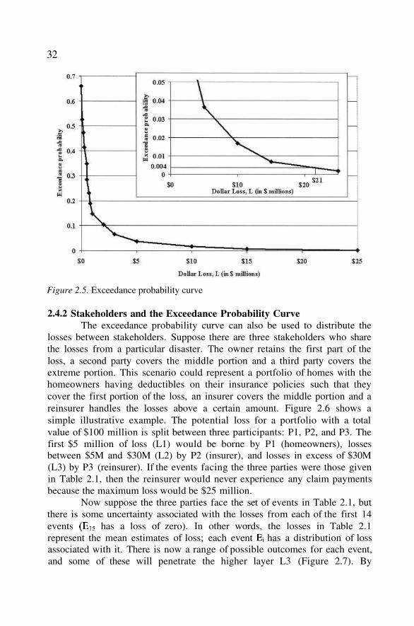
The resulting exceedance probability is the annual probability that theloss exceeds a given value. As seen in the equation above, this translates intoone minus the probability that all the other events below this value have notoccurred. The exceedance probability curve for the events in Table 2.1 isshown in Figure 2.5. Sidebar 1 explains how the EP curve can be used todetermine probable maximum loss (PML).

31

SIDEBAR 1: PML as a function of the EP CurveThe exceedance probability curve illustrated in Figure 2.5 enables an

insurer to determine his PML or Probable Maximum Loss for a portfolio ofstructures in a given time period. The term PML is a subjective risk metricand is associated with a given probability of exceedance specified by theinsurer. For example, suppose that an insurer specifies its acceptable risk levelas the 0.4% probability of exceedance. The insurer can use the EP curve todetermine how large a loss will occur at this probability level. Often, PMLlimits are framed in terms of a return period. The return period is simply theinverse of the annual probability of exceedance. In this example, a 1-in-250year PML is the lower limit on the loss at a 0.4% probability of exceedanceon the EP curve. From the inset of Figure 2.5, it can be seen that the PML isapproximately $21 million.

32

Figure 2.5. Exceedance probability curve

2.4.2 Stakeholders and the Exceedance Probability CurveThe exceedance probability curve can also be used to distribute the

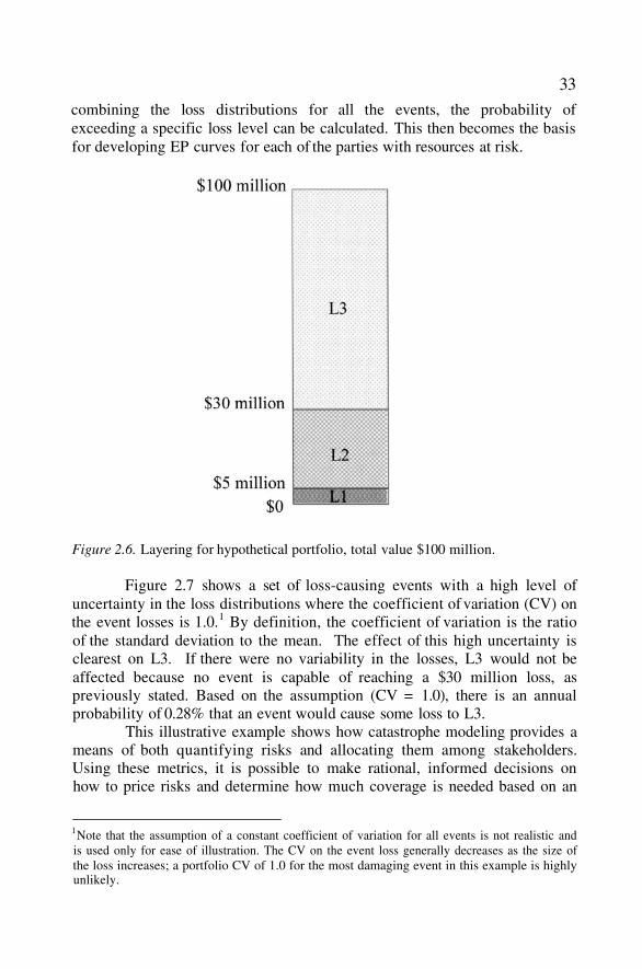
losses between stakeholders. Suppose there are three stakeholders who sharethe losses from a particular disaster. The owner retains the first part of theloss, a second party covers the middle portion and a third party covers theextreme portion. This scenario could represent a portfolio of homes with thehomeowners having deductibles on their insurance policies such that theycover the first portion of the loss, an insurer covers the middle portion and areinsurer handles the losses above a certain amount. Figure 2.6 shows asimple illustrative example. The potential loss for a portfolio with a totalvalue of $100 million is split between three participants: P1, P2, and P3. Thefirst $5 million of loss (L1) would be borne by P1 (homeowners), lossesbetween $5M and $30M (L2) by P2 (insurer), and losses in excess of $30M(L3) by P3 (reinsurer). If the events facing the three parties were those givenin Table 2.1, then the reinsurer would never experience any claim paymentsbecause the maximum loss would be $25 million.

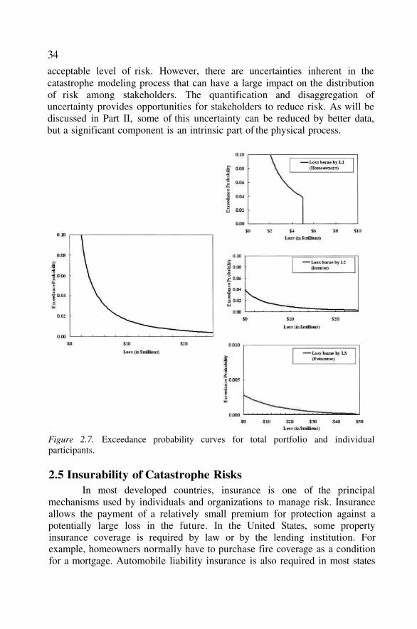
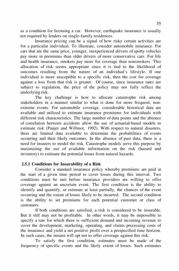
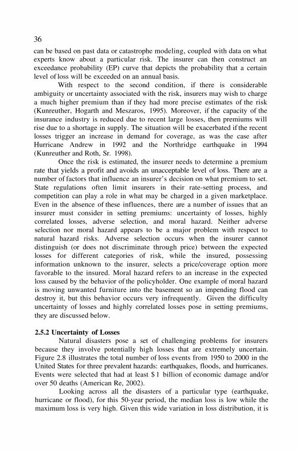
Now suppose the three parties face the set of events in Table 2.1, butthere is some uncertainty associated with the losses from each of the first 14events has a loss of zero). In other words, the losses in Table 2.1represent the mean estimates of loss; each event has a distribution of lossassociated with it. There is now a range of possible outcomes for each event,and some of these will penetrate the higher layer L3 (Figure 2.7). By

33

combining the loss distributions for all the events, the probability ofexceeding a specific loss level can be calculated. This then becomes the basisfor developing EP curves for each of the parties with resources at risk.

Figure 2.6. Layering for hypothetical portfolio, total value $100 million.

Figure 2.7 shows a set of loss-causing events with a high level ofuncertainty in the loss distributions where the coefficient of variation (CV) onthe event losses is 1.0.1 By definition, the coefficient of variation is the ratioof the standard deviation to the mean. The effect of this high uncertainty isclearest on L3. If there were no variability in the losses, L3 would not beaffected because no event is capable of reaching a $30 million loss, aspreviously stated. Based on the assumption (CV = 1.0), there is an annualprobability of 0.28% that an event would cause some loss to L3.

This illustrative example shows how catastrophe modeling provides ameans of both quantifying risks and allocating them among stakeholders.Using these metrics, it is possible to make rational, informed decisions onhow to price risks and determine how much coverage is needed based on an

1Note that the assumption of a constant coefficient of variation for all events is not realistic andis used only for ease of illustration. The CV on the event loss generally decreases as the size ofthe loss increases; a portfolio CV of 1.0 for the most damaging event in this example is highlyunlikely.

34

acceptable level of risk. However, there are uncertainties inherent in thecatastrophe modeling process that can have a large impact on the distributionof risk among stakeholders. The quantification and disaggregation ofuncertainty provides opportunities for stakeholders to reduce risk. As will bediscussed in Part II, some of this uncertainty can be reduced by better data,but a significant component is an intrinsic part of the physical process.

Figure 2.7. Exceedance probability curves for total portfolio and individualparticipants.

2.5 Insurability of Catastrophe RisksIn most developed countries, insurance is one of the principal

mechanisms used by individuals and organizations to manage risk. Insuranceallows the payment of a relatively small premium for protection against apotentially large loss in the future. In the United States, some propertyinsurance coverage is required by law or by the lending institution. Forexample, homeowners normally have to purchase fire coverage as a conditionfor a mortgage. Automobile liability insurance is also required in most states

35

as a condition for licensing a car. However, earthquake insurance is usuallynot required by lenders on single-family residences.

Insurance pricing can be a signal of how risky certain activities arefor a particular individual. To illustrate, consider automobile insurance. Forcars that are the same price, younger, inexperienced drivers of sporty vehiclespay more in premiums than older drivers of more conservative cars. For lifeand health insurance, smokers pay more for coverage than nonsmokers. Thisallocation of risk seems appropriate since it is tied to the likelihood ofoutcomes resulting from the nature of an individual’s lifestyle. If oneindividual is more susceptible to a specific risk, then the cost for coverageagainst a loss from that risk is greater. Of course, since insurance rates aresubject to regulation, the price of the policy may not fully reflect theunderlying risk.

The key challenge is how to allocate catastrophe risk amongstakeholders in a manner similar to what is done for more frequent, non-extreme events. For automobile coverage, considerable historical data areavailable and utilized to estimate insurance premiums for individuals withdifferent risk characteristics. The large number of data points and the absenceof correlation between accidents allow the use of actuarial-based models toestimate risk (Panjer and Willmot, 1992). With respect to natural disasters,there are limited data available to determine the probabilities of eventsoccurring and their likely outcomes. In the absence of past data, there is aneed for insurers to model the risk. Catastrophe models serve this purpose bymaximizing the use of available information on the risk (hazard andinventory) to estimate the potential losses from natural hazards.

2.5.1 Conditions for Insurability of a RiskConsider a standard insurance policy whereby premiums are paid at

the start of a given time period to cover losses during this interval. Twoconditions must be met before insurance providers are willing to offercoverage against an uncertain event. The first condition is the ability toidentify and quantify, or estimate at least partially, the chances of the eventoccurring and the extent of losses likely to be incurred. The second conditionis the ability to set premiums for each potential customer or class ofcustomers.

If both conditions are satisfied, a risk is considered to be insurable.But it still may not be profitable. In other words, it may be impossible tospecify a rate for which there is sufficient demand and incoming revenue tocover the development, marketing, operating, and claims processing costs ofthe insurance and yield a net positive profit over a prespecified time horizon.In such cases, the insurer will opt not to offer coverage against this risk.

To satisfy the first condition, estimates must be made of thefrequency of specific events and the likely extent of losses. Such estimates

36

can be based on past data or catastrophe modeling, coupled with data on whatexperts know about a particular risk. The insurer can then construct anexceedance probability (EP) curve that depicts the probability that a certainlevel of loss will be exceeded on an annual basis.

With respect to the second condition, if there is considerableambiguity or uncertainty associated with the risk, insurers may wish to chargea much higher premium than if they had more precise estimates of the risk(Kunreuther, Hogarth and Meszaros, 1995). Moreover, if the capacity of theinsurance industry is reduced due to recent large losses, then premiums willrise due to a shortage in supply. The situation will be exacerbated if the recentlosses trigger an increase in demand for coverage, as was the case afterHurricane Andrew in 1992 and the Northridge earthquake in 1994(Kunreuther and Roth, Sr. 1998).

Once the risk is estimated, the insurer needs to determine a premiumrate that yields a profit and avoids an unacceptable level of loss. There are anumber of factors that influence an insurer’s decision on what premium to set.State regulations often limit insurers in their rate-setting process, andcompetition can play a role in what may be charged in a given marketplace.Even in the absence of these influences, there are a number of issues that aninsurer must consider in setting premiums: uncertainty of losses, highlycorrelated losses, adverse selection, and moral hazard. Neither adverseselection nor moral hazard appears to be a major problem with respect tonatural hazard risks. Adverse selection occurs when the insurer cannotdistinguish (or does not discriminate through price) between the expectedlosses for different categories of risk, while the insured, possessinginformation unknown to the insurer, selects a price/coverage option morefavorable to the insured. Moral hazard refers to an increase in the expectedloss caused by the behavior of the policyholder. One example of moral hazardis moving unwanted furniture into the basement so an impending flood candestroy it, but this behavior occurs very infrequently. Given the difficultyuncertainty of losses and highly correlated losses pose in setting premiums,they are discussed below.

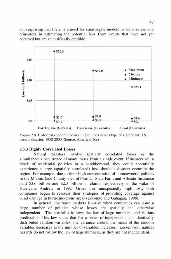
2.5.2 Uncertainty of LossesNatural disasters pose a set of challenging problems for insurers

because they involve potentially high losses that are extremely uncertain.Figure 2.8 illustrates the total number of loss events from 1950 to 2000 in theUnited States for three prevalent hazards: earthquakes, floods, and hurricanes.Events were selected that had at least $ 1 billion of economic damage and/orover 50 deaths (American Re, 2002).

Looking across all the disasters of a particular type (earthquake,hurricane or flood), for this 50-year period, the median loss is low while themaximum loss is very high. Given this wide variation in loss distribution, it is

37

not surprising that there is a need for catastrophe models to aid insurers andreinsurers in estimating the potential loss from events that have not yetoccurred but are scientifically credible.

Figure 2.8. Historical economic losses in $ billions versus type of significant U.S.natural disaster. 1950-2000 (Source: American Re)

2.5.3 Highly Correlated LossesNatural disasters involve spatially correlated losses or the

simultaneous occurrence of many losses from a single event. If insurers sell ablock of residential policies in a neighborhood, they could potentiallyexperience a large (spatially correlated) loss should a disaster occur in theregion. For example, due to their high concentration of homeowners’ policiesin the Miami/Dade County area of Florida, State Farm and Allstate Insurancepaid $3.6 billion and $2.3 billion in claims respectively in the wake ofHurricane Andrew in 1992. Given this unexpectedly high loss, bothcompanies began to reassess their strategies of providing coverage againstwind damage in hurricane-prone areas (Lecomte and Gahagan, 1998).

In general, insurance markets flourish when companies can issue alarge number of policies whose losses are spatially and otherwiseindependent. The portfolio follows the law of large numbers, and is thuspredictable. This law states that for a series of independent and identicallydistributed random variables, the variance around the mean of the randomvariables decreases as the number of variables increases. Losses from naturalhazards do not follow the law of large numbers, as they are not independent.

38

2.5.4 Determining Whether to Provide CoverageIn his study, James Stone (1973) sheds light on insurers’ decision

rules as to when they would market coverage for a specific risk. Stoneindicates that firms are interested in maximizing expected profits subject tosatisfying a constraint related to the survival of the firm. He also introduces aconstraint regarding the stability of the insurer’s operation. However, insurershave traditionally not focused on this constraint in dealing with catastrophicrisks.

Following the disasters of 1989, insurers focused on the survivalconstraint in determining the amount of catastrophe coverage they wanted toprovide. Moreover, insurers were caught off guard with respect to themagnitude of the losses from Hurricane Andrew in 1992 and the Northridgeearthquake in 1994. In conjunction with the insolvencies that resulted fromthese disasters, the demand for coverage increased. Insurers only marketedcoverage against wind damage in Florida because they were required to do soand state insurance pools were formed to limit their risk. Similarly, theCalifornia Earthquake Authority enabled the market to continue to offerearthquake coverage in California.

An insurer satisfies the survival constraint by choosing a portfolio ofrisks with an overall expected probability of insolvency less than somethreshold, A simple example illustrates how an insurer would utilize thesurvival constraint to determine whether the earthquake risk is insurable.Assume that all homes in an earthquake-prone area are equally resistant todamage such that the insurance premium, z, is the same for each structure.Further assume that an insurer has $A dollars in current surplus and wants todetermine the number of policies it can write and still satisfy its survivalconstraint. Then, the maximum number of policies, n, satisfying the survivalconstraint is:

Whether the company will view the earthquake risk as insurabledepends on whether the fixed cost of marketing and issuing policies issufficiently low to make a positive expected profit. This, in turn, depends onhow large the value of n is for any given premium, z. Note that the companyalso has some freedom to change its premium. A larger z will increase thevalues of n but will lower the demand for coverage. The insurer will decidenot to offer earthquake coverage if it believes it cannot attract enough demandat any premium structure to make a positive expected profit. The companywill use the survival constraint to determine the maximum number of policiesit is willing to offer.

The EP curve is a useful tool for insurers to utilize in order toexamine the conditions for meeting their survival constraint. Suppose that an

39

insurer wants to determine whether its current portfolio of properties in LongBeach is meeting the survival constraint for the earthquake hazard. Based on

its current surplus and total earthquake premiums, the insurer is declaredinsolvent if it suffers a loss greater than $ 15 million. The insurer can constructan EP curve such as Figure 2.4 and examine the probability that losses exceed

certain amounts. From this figure, the probability of insolvency is 1.0%. Ifthe acceptable risk level, then the insurer can either decrease theamount of coverage, raise the premium and/or transfer some of the risk to

others.

2.6 Framework to Integrate Risk Assessment with RiskManagement

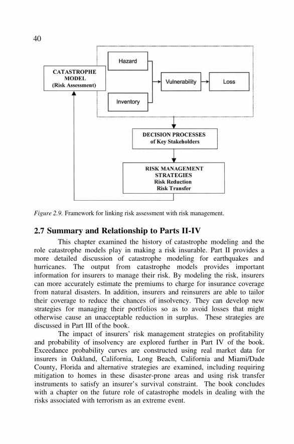
Figure 2.9 depicts a framework for integrating risk assessment withrisk management and serves as a guide to the concepts and analyses presentedin this book. The risk is first assessed through catastrophe modeling.Catastrophe modeling combines the four components (hazard, inventory,vulnerability, and loss) to aid insurers in making their decisions on what typeof protection they can offer against a particular risk.

The key link between assessing risk via catastrophe models andimplementing risk management strategies is the stakeholders’ decisionprocesses. The types of information stakeholders collect and the nature oftheir decision processes are essential in developing risk managementstrategies. With respect to insurers, catastrophe models are the primarysources of information on the risk. Their decision rule for developing riskmanagement strategies is to maximize expected profits subject to meeting thesurvival constraint. Property owners in hazard prone areas utilize simplifieddecision rules in determining whether or not to adopt mitigation measures toreduce future losses to their property and/or to purchase insurance.

For purposes of this book, risk management strategies are broadlyclassified as either risk reduction measures, such as mitigation, or risk transfermeasures, such as reinsurance. For example, strategies for residential propertyowners often involve a combination of measures, including mitigation,insurance, well-enforced building codes, and land-use regulations. In Californiaand Florida, all these initiatives exist in some form. Strategies for insurers couldinvolve charging higher rates to reflect the uncertainty of the risk, changing theirportfolio so they can spread the risk across many areas, or reassigning the riskusing risk transfer instruments such as reinsurance and/or catastrophe bonds.

40

Figure 2.9. Framework for linking risk assessment with risk management.

2.7 Summary and Relationship to Parts II-IVThis chapter examined the history of catastrophe modeling and the

role catastrophe models play in making a risk insurable. Part II provides amore detailed discussion of catastrophe modeling for earthquakes andhurricanes. The output from catastrophe models provides importantinformation for insurers to manage their risk. By modeling the risk, insurerscan more accurately estimate the premiums to charge for insurance coveragefrom natural disasters. In addition, insurers and reinsurers are able to tailortheir coverage to reduce the chances of insolvency. They can develop newstrategies for managing their portfolios so as to avoid losses that mightotherwise cause an unacceptable reduction in surplus. These strategies arediscussed in Part III of the book.

The impact of insurers’ risk management strategies on profitabilityand probability of insolvency are explored further in Part IV of the book.Exceedance probability curves are constructed using real market data forinsurers in Oakland, California, Long Beach, California and Miami/DadeCounty, Florida and alternative strategies are examined, including requiringmitigation to homes in these disaster-prone areas and using risk transferinstruments to satisfy an insurer’s survival constraint. The book concludeswith a chapter on the future role of catastrophe models in dealing with therisks associated with terrorism as an extreme event.

41

2.8 References

American Re (2002). Topics: Annual Review of North American NaturalCatastrophes 2001.

Algermissen, S.T. (1969). Seismic risk studies in the United States, 4th WorldConference on Earthquake Engineering Proceedings, Chilean Association forSeismology and Earthquake Engineering, Santiago, Chile.

Brinkmann, W. (1975). Hurricane Hazard in the United States: A ResearchAssessment. Monograph #NSF-RA-E-75-007, Program on Technology, Environmentand Man, Institute of Behavioral Sciences, University of Colorado, Boulder,Colorado.

FEMA 249 (1994). Assessment of the State of the Art Earthquake Loss EstimationMethodologies, June.

FEMA (2002). HAZUS99 SR2 User’s Manual, Federal Emergency ManagementAgency.

Insurance Information Institute (2000). Catastrophes [online]. The InsuranceInformation Institute 10 June 2000 <http://www.iii.org/media/issues/catastrophes>.

Kozlowski, R. T. and Mathewson, S. B. (1995). “Measuring and ManagingCatastrophe Risk,”1995 Discussion Papers on Dynamic Financial Analysis, CasualtyActuarial Society, Arlington, Virginia.

Kunreuther, H., R. Hogarth, J. Meszaros and M. Spranca (1995). “Ambiguity andunderwriter decision processes,” Journal of Economic Behavior and Organization,26: 337-352.

Kunreuther, H. and Roth, R. (1998). Paying the Price: The Status and Role ofInsurance Against Natural Disasters in the United States. Washington, D.C: JosephHenry Press.

Neumann, C.J. (1972). An alternate to the HURRAN tropical cyclone forecast system.NOAA Tech. Memo. NWS SR-62, 24 pp.

NIBS (1997). HAZUS: Hazards U.S.: Earthquake Loss Estimation Methodology. NIBSDocument Number 5200, National Institute of Building Sciences, Washington, D.C.

Panjer, H. H. and Willmot, G.E. (1992). Insurance Risk Models. Illinois: Society ofActuaries.

Steinbrugge, K. V. (1982). Earthquakes, Volcanoes, and Tsunamis: An Anatomy ofHazards. Skandia America Group: New York, New York.

42

Stone, J. (1973). “A theory of capacity and the insurance of catastrophe risks: Part Iand Part II,” Journal of Risk and Insurance, 40: 231-243 (Part I) and 40: 339-355(Part II).

Stover, C.W. and Coffman, J.L (1993). Seismicity of the United States, 1568-1989.U.S. Geological Survey Professional Paper 1527, United States Government PrintingOffice, Washington, D.C.

USWRC (1967). A Uniform Technique for Determining Flood Flow Frequencies,U.S. Water Resource Council, Hydrology Committee, Bulletin 15, Washington, D.C.